| Issue |
A&A
Volume 575, March 2015
|
|
|---|---|---|
| Article Number | A91 | |
| Number of page(s) | 11 | |
| Section | Interstellar and circumstellar matter | |
| DOI | https://doi.org/10.1051/0004-6361/201424565 | |
| Published online | 03 March 2015 | |
Molecular shells in IRC+10216: tracing the mass loss history⋆,⋆⋆,⋆⋆⋆
1 ICMM. CSIC. Group of Molecular Astrophysics. C/ Sor Juana Inés de la Cruz 3. Cantoblanco, 28049 Madrid, Spain
e-mail: This email address is being protected from spambots. You need JavaScript enabled to view it.
2 National Radio Astronomy Observatory, 520 Edgemont Road, Charlottesville, VA 22903, USA
3 Institut de Radioastronomie Millimétrique, 300 rue de la Piscine, 38406 Saint Martin d’Hères, France
4 LERMA, Observatoire de Paris, PSL Research University, CNRS, UMR 8112, 75014 Paris, France
Received: 9 July 2014
Accepted: 5 December 2014
Abstract
Thermally-pulsating AGB stars provide three-fourths of the matter returned to the interstellar medium. The mass and chemical composition of their ejecta largely control the chemical evolution of galaxies. Yet, both the mass loss process and the gas chemical composition remain poorly understood. We present maps of the extended 12CO and 13CO emissions in IRC+10216, the envelope of CW Leo, the high mass loss star the closest to the Sun. IRC+10216 is nearly spherical and expands radially with a velocity of 14.5 km s-1. The observations were made On-the-Fly with the IRAM 30 m telescope; their sensibility, calibration, and angular resolution are far higher than all previous studies. The telescope resolution at λ = 1.3 mm (11′′ HPBW) corresponds to an expansion time of 500 yr. The CO emission consists of a centrally peaked pedestal and a series of bright, nearly spherical shells. It peaks on CW Leo and remains relatively strong up to rphot = 180′′. Further out the emission becomes very weak and vanishes as CO gets photodissociated. As CO is the best tracer of the gas up to rphot, the maps show the mass loss history in the last 8000 yr. The bright CO shells denote over-dense regions. They show that the mass loss process is highly variable on timescales of hundreds of years. The new data, however, do not support previous claims of a strong decrease of the average mass loss in the last few thousand years. The over-dense shells are not perfectly concentric and extend farther to the N-NW. The typical shell separation is 800−1000 yr in the middle of the envelope, but seems to increase outwards. The shell-intershell brightness contrast is ≥3. All those key features can be accounted for if CW Leo has a companion star with a period ≃800 yr that increases the mass loss rate when it comes close to periastron. Higher angular resolution observations are needed to fully resolve the dense shells and measure the density contrast. The latter plays an essential role in our understanding of the envelope chemistry.
Key words: astrochemistry / stars: AGB and post-AGB / circumstellar matter / stars: individual: IRC+10216
This work was based on observations carried out with the IRAM 30 m telescope. IRAM is supported by INSU/CNRS (France), MPG (Germany) and IGN (Spain).
Movies associated to Figs. 3, 5, 7, 8, and 10 are available in electronic form at http://www.aanda.org
Data cubes as FITS files are only available at the CDS via anonymous ftp to cdsarc.u-strasbg.fr (130.79.128.5) or via http://cdsarc.u-strasbg.fr/viz-bin/qcat?J/A+A/575/A91
© ESO, 2015
1. Introduction
The mass and chemical composition of stellar ejecta are keys to our understanding of Galactic chemical evolution. The main source of ejecta are Supernova explosions and asymptotic giant branch (AGB) star winds. The latter, in particular, the winds of thermally pulsing AGB (TP-AGB) stars, provide as much as three-quarters of the matter returned to the interstellar medium (ISM; Gehrz 1989). During their phase of high mass loss, the envelopes become opaque at optical and near-IR wavelengths; their hot, innermost parts are then best studied in the mid- and far-IR (FIR) and their cool outer parts at millimeter wavelengths.
IRC+10216, the thick dusty envelope of CW Leo and the TP-AGB star the closest to the Sun, is a choice target for these studies. Its C-rich nature was pointed out by Herbig & Zappala (1970) who assigned a cool N type for the star (C9.5). Besides its proximity (≃130 pc), IRC+10216 is remarkable in several respects: a large mass (~2 M⊙) and apparent size (6′), a nearly spherical shape and constant expansion velocity, except near the star, and, last but not least, an incredible wealth of molecular species: half of the known interstellar species are observed in its C-rich outer envelope. These molecules range from CO, the main tracer of the cool molecular gas and other diatomic and triatomic species (see e.g. Cernicharo et al. 2000, 2010), to refractory element molecules (Cernicharo & Guélin 1987), the last detected molecule being HMgNC (Cabezas et al. 2013), to long carbon chains species CnH (Cernicharo & Guélin 1996; Guélin et al. 1997, and references therein), and include all known interstellar anions (C2nH−, n = 2,3,4 and C2n+1N−, n = 0,1,2, Thaddeus et al. 2008; Cernicharo et al. 2008, and references therein).
In addition to this large list of molecules expected in a carbon-rich environment, oxygen-bearing species such as H2O (Melnick et al. 2001), OH, and H2CO (Ford et al. 2003, 2004) have been also detected. While the presence of H2O and H2CO in more evolved C-rich protoplanetary nebula can be easily explained through photochemical processes (Cernicharo 2004), their presence in IRC+10216, a star still in the AGB phase, is particularly difficult to explain. Agúndez et al. (2010) have shown that an important parameter for the chemical models is the spatial structure of the gas in the circumstellar envelope (CSE) which, if clumpy enough, could permit the interstellar UV radiation to penetrate into the inner zones of the CSE and trigger a chemistry out of thermodynamical equilibrium.
Although at low angular resolution the mm-wave dust and CO emissions of IRC+10216 appear fairly smooth and spherically symmetric, high resolution V-light images of the envelope (Crabtree et al. 1987; Mauron & Huggins 1999, 2000; Leao et al. 2006), and emission maps of reactive molecular species (Guélin et al. 1999; Trung & Lim 2008) reveal multiple shell-like structures that seem to reflect recurrent episodes of high mass loss with timescales of hundreds of years. The shells appear patchy and broken into pieces, but are fairly spherical in the r = 15 − 30′′ radius region. Surprisingly, they are not exactly centred on CW Leo, but a couple of arcsec away (Guélin et al. 1993). Emission from reactive species is weaker at PA ≃ + 20° and −160° (Lucas et al. 1995), suggesting that CW Leo may be leaving the AGB and is developing a bipolar outflow that sweeps away parts of the slowly expending spherical envelope. Further evidence of matter ejection along the PA = −20 − + 160° axis comes from the SiS brightness contours (Lucas et al. 1995), which show that the 4′′ diameter envelope core, as traced by SiS molecules is elongated in that direction.
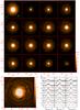 |
Fig. 1 Top left box: velocity-integrated CO (J = 2−1) line emission in the central 400′′ × 400′′ area (VLSR range from −41 to −12 km s-1). Other upper maps: velocity-channel maps (resolution 2 km s-1); marked velocities are relative to the LSR systemic star velocity (V∗ = −26.5 km s-1); the units of the color scale correspond to K km s-1. Positive and negative velocities correspond to the rear and front parts of the envelope, respectively. Bottom right panels: observed 12CO(2−1) line profiles along a strip to the east for Δδ = 0′′; the upper left numbers indicate Δα in arcseconds and the upper right numbers the intensity scaling factor applied to plot all spectra at the same |
At small angular scales the images obtained by Kastner & Weintraub (1994) and Skinner et al. (1998) show deviations from symmetry suggesting the presence of an overall bipolar structure. Moreover, high angular resolution observations of the continuum indicate the presence of clumps and show that the innermost structures at subarsecond scale are changing on timescales of years (Haniff & Buscher 1998; Monnier et al. 2000; Men’shchikov et al. 2001; Tuthill et al. 2000). All these fast variations in recent years led several authors, following Lucas et al. (1995), to suggest that CW Leo is beginning its evolution towards the protoplanetary nebula phase (Tuthill et al. 2000, and references therein).
More recently, Decin et al. (2011) reported Herschel/PACS maps of the dust FIR emission showing that the dusty shells observed in V-light extend in the envelope up to radii R ≥ 3′. Although it was known, from low-resolution studies, that CO emission extends at least as far, little was known so far about the gas distribution at such radii, more particularly in the region where CO is photodissociated by interstellar (IS) UV radiation. Moreover, contrary to dust, CO yields the velocity information needed to reconstruct the 3D envelope structure. Fong et al. (2003), who mapped the emission up to R = 150′′ with BIMA (13′′ synthetized beam), reported the presence of a number of arc-shaped features apparently associated with the thin dust shells reported by Mauron & Huggins (2000). However, the limited size and low sensitivity of the BIMA map prevented them from drawing an image of the full envelope. To derive the molecular gas distribution up to at least 4′ from the star and investigate CW Leo’s mass loss history over the last 104 years, we have observed with high sensitivity the 12CO and 13CO J = 2−1 line emissions throughout the envelope, using the HERA focal plane array receiver on the IRAM 30 m telescope. The half-power beamwidth (HPBW) of the telescope, 11′′, or 1400 AU, is small enough to resolve clumps of gas expelled with a 500 yr delay1.
2. Observations
The main observations of 12CO and 13CO J = 2−1 (see Fig. 1) were carried out in February 2009 with the HERA 9 pixel, dual-polarization receiver on the IRAM 30 m telescope (Schuster et al. 2004). Further observations of 12CO and 13CO J = 1−0 and 2−1 were made between 2011 and 2012, using the Eight MIxer Receiver (EMIR): E90 and E230 single-pixel dual polarization receivers.
The astronomical signals are expressed in the  , scale (antenna temperature corrected for spillover losses and atmospheric opacity) in Figs. 1 and 2, and in the TMB scale in the subsequent figures (TMB = TA/Beff, where Beff, the telescope beam efficiency is 0.79, 0.78, 0.61, and 0.59 at 110 GHz, 115 GHz, 220 GHz, and 230 GHz, respectively: Kramer et al. 2013). The atmospheric opacity was measured from the comparison of the sky emissivity, recorded every five minutes, to that of hot and cold loads using the ATM code (Cernicharo 1985; Pardo et al. 2001).The zenith sky opacity was typically 0.1−0.2. The spectral data were processed by an autocorrelator consisting of 461 channels spaced by 312 KHz (0.41 km s-1 at 230.5 GHz).
The nine sky-channels of HERA of each linear polarization were successively tuned to the frequencies of J = 2−1 12CO and J = 2−113CO lines. The receivers operated in single sideband mode, with image rejections ≥10 dB. The observations were made in the On-The-Fly mode by mapping nine partly overlapping areas of size 240′′ × 240′′. Each map consisted in constant declination scans, separated in declination by 4′′ (for the central map) or 6′′ (for the other maps). The scanning velocity was 8′′ per second and the data dumped every 0.15 s, yielding one spectrum every 1.2′′ in RA. The observing time per individual map was ≃1 h.
The first map was centred at 0,0, i.e. on the star CW Leo, maps 2−5 at (+ 240′′,0) (−240′′,0) (0, + 240′′) and (0, −240′′). Maps 6−9, of size 120′′ × 120′′, were centred at (+180′′, + 180′′) (+ 180′′, − 180′′) (−180′′, +180′′), and (−180′′, −180′′). The combined map fully samples a square area of size 480′′ × 480′′, centred on the star. Four additional 240′′ × 240′′ areas, centred on the four corners of the square and extending up to ± 720′′ from the star, were also observed.
Prior to observing each individual map, the pointing and focus of the telescope were checked on the quasar OJ287. In addition, a small mini-map centred on the star, was observed with HERA in the position switching mode for further checks of calibration and pointing. The coordinates adopted for position (0,0) are α2000 = 09h47m57.3s , δ2000 = 13°16′43.3′′. The telescope HPBW was 11′′ and 22′′, respectively, for the 12CO J = 2−1 and J = 1 − 0 lines, and 11.5′′ and 23′′ for the 13CO J = 2−1 and J = 1 − 0 lines.
The relative positions of the 9 × 2 sky-channels of HERA were measured on the first (0,0) map. There, the star and its surroundings appear in CO emission as a bright compact source. We found shifts of up to 2′′ from the nominal channel positions. We measured the relative calibration of the 9 × 2 channels of HERA; differences of up to 20% were found. The shifts and correction factors were applied and the data re-sampled on a common grid with Δα = Δδ = 2′′ before merging the different sky and polarization channels into a single map. The rms noise per 0.4 km s-1-wide channel, after averaging overlapping maps and both polarizations over a grid with points separated every 2′′, varies between 0.14 K in the central positions and 0.06 K at the map borders (± 240′′, ± 240′′).
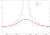 |
Fig. 2 Black line: intensity of the 12CO(2−1) line integrated between LSR velocities −25.5 and −27.5 km s-1 observed along an EW strip at the declination of the star (Δδ = 0′′). Red line: the response of the telescope error beam to the 12CO(2−1) emission along the same strip. The error beam consists of 3 Gaussians of full width at half power (FWHP) 65′′, 250′′, and 860′′ and intensities 1.9 × 10⁻³, 3.5 × 10⁻⁴, and 2.2 × 10⁻⁵ relative to the main beam, respectively. Blue line: the 12CO(2−1) line intensity after removal of the error beam response. |
The EMIR observations consisted of a partial map of 13CO J = 1 − 0 emission, and of deep integrations of 12CO J = 2−1, 1−0 along selected strips. The EMIR 13CO J = 2−1 and 1−0 and 12CO J = 1 − 0 data were observed in the raster mode and consisted of maps of 120 × 120′′ and of strips extending up to ± 720′′ from the star (reference position was 15 arcmin west from the star). The typical rms noise per channel of 0.4 km s-1 is 0.06 K. These data are used in Sect. 3.1 to derive the gas physical properties through the envelope.
The 30 m telescope response to point sources is not restricted to a Gaussian beam with (FWHP of 11′′), but includes near side-lobes and an error beam. The latter has been measured at 230 GHz and at 115 GHz and contains 25% and 14%, respectively, of the energy collected by the telescope, and extends over the entire IRC+10216 envelope. At 230 GHz, it can be approximated by 3 Gaussians with FWHP of 65′′, 250′′, and 860′′ (Kramer et al. 2013). The signals observed at position (0,0) are then significantly affected by the response of the error beam to the outer envelope and those observed in the outer envelope are affected by the compact central source. Since our map fully covers the bulk of the envelope CO emission (whose diameter is ≤400′′), we were able to correct the response of the error beam in every velocity-channel at each observed position. The error-beam corrected velocity-channel maps are shown in Fig. 1 for the central 400′′ × 400′′ region. Figure 2 shows the 12CO(2−1) intensities prior to and after this correction along a cut at the declination of the central star. The contribution of the error beam at the frequencies of the J = 1 − 0 lines of 12CO and 13CO is much less important as this beam is weaker and broader, and has not been removed from the data.
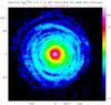 |
Fig. 3 Main beam-averaged 12CO(2−1) line brightness temperature observed at VLSR − V∗ = 0 km s-1 (Δv = 0.1 km s-1). This is the central frame of a video showing the distribution of the 12CO line emission at different velocities (online). |
Finally, Fig. 3 shows the central frame of a video (online) showing the spatial distribution of the CO emission at different velocities. The CO data have been re-sampled to a velocity resolution of 0.1 km s-1, and hence, there is a significant correlation between consecutive frames in the online video.
3. Results and discussion
Given that the outer envelope is in expansion with a constant velocity of 14.5 km s-1, each velocity-channel map of Figs. 1 and 3 delineates a conical sector (of opening θ and thickness δθ), whose axis is aligned with the line of sight to the star CW Leo. The extreme velocities correspond to the approaching and receding polar cones and caps, while the middle velocity (v = VLSR − V ∗ = 0 km s-1, where V ∗ is the star LSR velocity, V ∗ = −26.5 km s-1) corresponds to a cut through the star in the plane of the sky.
The multiple shell structure traced by the CO(2−1) emission near v = 0 km s-1 is spectacular. It consists of at least seven distinct shells of radii ranging from r = 45′′ to r = 170′′ and with a fairly high shell-intershell brightness contrast. We know from interferometric maps of reactive molecules (Guélin et al. 1999; Trung & Lim 2008), as well as from V-band images of scattered light, that more shells or pieces of shell are present at smaller radii: r ≃ 16′′, 25′′ and 35′′. Those are, however, too tight and/or too close to the bright central source to be resolved by the 11′′ telescope beam. The shells in Fig. 1 seem fairly spherical, albeit not necessarily centred on CW Leo. Some are locally flattened. A nice spiral structure may be seen at velocities ±8 and ±10 km s-1 , which suggests, as discussed below and already indicated by Guélin et al. (1993), that CW Leo is a binary star with its orbital plane near to a face-on view. As a result of off-centring, the shells intersect at several places, possibly a projection effect, tracing a pattern reminiscent of the rose-window filaments observed by the HST in a number of planetary nebulae (Balick & Frank 2002, and references therein).
Obviously, the outer shell pattern teaches us about the mass loss history during the past 104 yr. It tells us how the envelope expanded and how far it is penetrated by IS UV radiation, which is a powerful booster of radical-neutral chemistry.
3.1. Mass loss history
We may estimate the masses of the envelope from the line brightness of key molecules in three different ways.
- I)
The first method focusses on lines from molecules formed in the upper atmosphere of the star: CO, HCCH, HCN (Cernicharo et al. 1996; Fonfría et al. 2008). The initial abundances of those “parent” molecules, x0, can be estimated from thermochemical equilibrium calculations (see e.g. Agúndez et al. 2010). In C-rich envelopes, the abundance of CO is close to that of oxygen and remains stable up to the CO photodissociation region (see below). Agúndez et al. (2012) analysed the shapes and intensities of many CO rotational lines, arising from widely different energy levels, using parametrized models of the inner envelope and a radiative transfer code. They assumed spherical symmetry and used the LVG approximation. For x0 = CO/H2 = 6 × 10⁻⁴, these authors derived the physical conditions in the inner envelope. Their density profile for r ≤ 10′′ yields an average mass loss rate Ṁt0 ≃ 2 × 10⁻⁵ M⊙ for the last 500 yr.
- II)
The second method relies on the measurement of the CO photodissociation radius, rphot, defined as the radius where the CO abundance has decreased by a factor of 2: x(CO) = x0/2 (see e.g. Morris & Jura 1983; Mamon et al. 1988; Stanek et al. 1995; Doty et al. 1995; Schöier & Olofsson 2001). It assumes that the surrounding interstellar (IS) UV field is known. Most authors adopt the IS radiation field of Jura (1974), which yields in the absence of shielding a CO photodissociation rate of G0 = 2 × 10¹⁰ s-1 (see Table 1 of Mamon et al. 1988). The method also assumes that the gas density decreases as r-2 in the outermost envelope layers and is not too clumpy. Figure 1 shows that the 12CO(2−1) emission extends up to r ≃ 180′′ (or 3.6 × 1017 cm) and becomes vanishingly small afterwards. Adopting this radius for the photodissociation radius rphot, we find a mass loss rate Ṁt ≃ 2 × 10⁻⁵ M⊙ (see Table 3 of Mamon et al. 1988). Obviously, this method yields the average mass loss rate at times t>t0 − rphot/vexp, i.e. more than 8 × 10³ yr ago.
- III)
The last method is based on 13CO. It assumes that, for r ≪ rphot, the 12CO and 13CO fractional abundances remain constant and close to their nominal values near the star, x0. This is expected since the CO molecule is chemically stable because 12CO efficiently self-shields against photodissociation and partially shields 13CO, and because both species are partially shielded by H2. As a matter of fact, the photodissociation radii of both isotopologues are similar (Mamon et al. 1988). As for 13C fractionation, it should be inefficient in IRC+10216 since, contrary to PNs (e.g. CRL618, Pardo & Cernicharo 2007) and detached envelopes (e.g. RScu, Vlemmings et al. 2013), the degree of ionization is known to be low in this envelope (see Mamon et al. 1988, for a discussion of CO shielding, isotopic fractionation, and selective photodissociation in dense CSEs). Finally, the chances that thermal pulses have changed the 13C/12C ratio during the last 8000 years are low (Nollett et al. 2003). Hence, the 13CO/12CO abundance ratio is expected to remain constant within rphot and close to the elemental 13C/12C ratio. Molecular line observations do point towards a single value 13CO/12CO = 13C/12C = 45 ± 3 with no change of the 13C/12C ratio between the inner and the outer parts of the IRC+10216 envelope (Kahane et al. 1988; Cernicharo et al. 1991, 2000). From the 12CO abundance derived through method (I) above, x0(12CO) = 6 × 10⁻⁴, we derive a 13CO fractional abundance x(12CO) = 1.3 × 10⁻⁵.
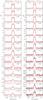 |
Fig. 4 Left panel: 13CO J = 1 − 0 and J = 2−1 line profiles (black and red histograms, respectively), averaged over concentric rings of width Δr = 10′′, observed at radii ranging from r = 0′′ to 130′′. The ordinate scale (black numbers) applies to the J = 1 − 0 line profile (black). The number in red in the upper left corner is the factor by which the J = 2−1 profile (red) has been divided to match the intensity scale. For r< 90′′ it also represents the R21 = 13CO(2−1)/13CO(1−0) velocity-integrated line intensity ratio. Right panel: J = 2−112CO (black) and 13CO line profiles averaged over the same 10′′-wide rings. The ordinate scale applies to the 13CO(2−1) line profile (red). The number in black in the upper left corner is the factor by which the 12CO(2−1) profile (black) has been divided to match the intensity scale. For r ≥ 40′′, it also represents the Ri = 12CO(2−1)/13CO(2−1) velocity-integrated line intensity ratio. |
Figure 4 shows the line profiles observed between r = 0 and r = 130′′ along a strip at the declination of the star. To increase the signal-to-noise ratio, the 13CO(2−1) and 12CO(2−1) line intensities of Fig. 1 have been averaged in azimuth over 10′′ wide concentric rings. The numbers in the upper left corner of each spectrum indicate the scaling ratio between the black and red line profiles (e.g. the 12CO(2−1) and 13CO(2−1) profiles). They give the  CO (2−1)/13CO(1−0) and
  CO(2−1)/13CO(2−1) velocity-integrated intensity ratios directly, where the black and red line profiles have similar shapes and intensities (i.e. at radii r ≤ 90′′ for the left panels and r ≥ 50′′ for the right panels).
We have fitted with a LVG radiative transfer code included in the MADEX code (Cernicharo 2012), the intensities of the 12CO and 13CO J = 2−1 and 1−0 lines at different radii. We find that the kinetic gas temperatures Tk derived for the successive rings of Fig. 4 are compatible with the temperature profile Tgas ∝ r-0.54 given by Agúndez & Cernicharo (2006), albeit ≃20% higher. From our multi-line analysis, we find for example at r = 40′′,60′′, and 80′′ (corresponding to evolution times of 1700, 2600 and 3400 yr, respectively), n(H2) ≃ 5 × 10³, 2.2 × 10³ and 1.2 × 103 cm-3, Tk ≃ 20 K, 16 K, and 13 K. The resulting mass loss rates are all Mt ≃ 4 × 10⁻⁵ M⊙, with an uncertainty of a factor of ≃2 (mainly resulting from the temperature-density near degeneracy and the uncertainty on the error beam contribution at large radii, from the difference in beamsizes at 115 GHz and 230 GHz at small radii, and from the uncertainty on the 13CO fractional abundance). For r = 120′′ we find Mt = 3.5 × 10⁻⁵ M⊙. These mass loss rates are within the uncertainties equal to those quoted above for r< 10′′ and r> 180′′.
Our study shows that the 12CO(2−1) line is very thick at small radii, and moderately thick (τ = 4 − 2) at radii larger than 40′′. The 13CO lines are optically thin (≤0.1), and the (2−1) 12CO and 13CO lines sub-thermally excited at radii r ≥ 40′′. The (2−1) line excitation becomes very low for r ≥ 90′′, where the average 12CO(2−1) line brightness temperature drops below 1 K and the R21 = 13CO(2−1)/13CO(1−0) ratio drops below 1. We note that the LVG models fail to reproduce the 12CO(2−1) line intensities and the  CO(2−1)/13CO(2−1) intensity ratio of Fig. 4, both of which are a factor of 2−3 times smaller than predicted for 40′′ ≤ r ≤ 80′′. This results from an underestimation of the 12CO line opacity because of the presence of dense sub-structures in the shells. These structures appear on high-resolution interferometric CO maps (Guélin et al., in prep.), as well as on the visible-light images (e.g. Leao et al. 2006). They are unresolved by the 11′′ telescope beam and smoothed out by our azimuthal averages. They probably contain a fair fraction of the total gas mass and significantly contribute to the optically thin 13CO emission, albeit they contribute little to the optically thick 12CO(2−1) emission, which is damped. The relatively low 12CO intensities could also result from a decrease of the 12CO/13CO abundance ratio at radii ≥40′′; however, selective photodissociation and thermal pulses, which are the mechanisms the most likely to affect this ratio, should increase, rather than decrease the 12CO/13CO ratio, making this explanation unlikely. Finally, although the J = 2−1 CO lines are much less sensitive to radiative IR pumping than the J = 3 − 2 and 1−0 lines, the effect is not negligible and may affect both R21 and Ri (see e.g. Cernicharo et al. 2014). Even though the observed values of the 12CO/13CO intensity ratio are low, they follow the predicted behaviour: high at small radii, where 12CO(2−1) is optically very thick, they are a minimum of between r = 30′′ and 60′′ and strongly increase at r> 100′′. As for the R21 line intensity ratio, it is accurately reproduced by our LVG calculations.
The result of our investigation is that the mass loss rate, averaged over periods longer than the periodic modulation that gives rise to the dense shells, seems within a factor of 2 constant over the last 104 years. Integrated over the range r∗ ≤ r ≤ 180′′, it yields an envelope mass M(rphot) = 0.3 M⊙. The total mass lost by the star since it joined the AGB phase can be estimated to be ≃2 M⊙ from the first shell ejected 70 000 yr ago (Sahai & Chronopoulos 2010).
Prior to our investigation, several attempts have been made to estimate the mass loss rate and the envelope mass. Crosas & Menten (1997) and De Beck et al. (2012) used mm and sub-mm lines of 12CO and 13CO, observed towards CW Leo or near this star, to derive a mass-loss rate averaged along the line of sight. They found values within a factor of 2 equal to ours. Other attempts were based on the dust thermal emission. Decin et al. (2011) derived from the Herschel/PACS 100 μm flux, after removing the background emission, an envelope mass of 0.23 M⊙ inside a 390′′ radius. For a distance of 130 pc and an expansion velocity of 14.5 km s-1, this corresponds to an average mass loss rate Ṁ = 1.4 × 10⁻⁵ M⊙ yr-1 over the last 1.7 × 10⁴ yr. Those values, however, depend heavily on the assumed dust temperature profile, since the 100 μm dust emission varies as  (100 μm is close to the peak of the dust emission for Td ≃ 30 K, the average temperature in the outer envelope). They also depend on the dust emissivity coefficient and dust-to-gas mass ratio (assumed equal to 250), two parameters uncertain by factors of a few. Obviously, they depend on the accuracy of the 100 μm flux measurement, which are uncertain by a factor ≥2 because of point spread function (PSF) artefacts (Decin et al. 2011). In view of all those uncertainties, the mass loss rate derived by Decin and coworkers is remarkably close to that we derive from CO.
Neither the high quality and high resolution CO data reported here and the FIR data from Herschel/PACS support earlier findings, based on balloon or IRAS FIR data, that the average mass-loss rate has strongly decreased in the past few thousand years (by a factor of 2 in the past 2000 yr, according to Fazio et al. 1980; and by a factor of 9 in the past 7000 yr, according to Groenewegen 1997). From an analysis of all the CO data available in 1998, using an elaborated source and radiative transfer models, Groenewegen et al. (1998) also advocated a decrease of Ṁ by a factor of 5 in the last 3000 yr. However, as pointed out by these authors, the IRAS and balloon observations lacked either angular resolution or spectral coverage, while the CO data available at that time for the outer envelope were widely discrepant. Our 30 m telescope data and the HIFI and PACS data benefit from a higher sensitivity and angular resolution. Our CO maps were observed by good weather, mostly through fast on-the-fly scanning, and are certainly much more homogeneous and more reliable than those used by Groenewegen and collaborators. We note that Teyssier et al. (2006), from a relatively recent analysis of the 12CO(1−0) through (6−5) lines, arrived at Ṁ = 1.2 × 10⁻⁵ M⊙ yr-1 (1.8 × 10⁻⁵ M⊙ yr-1 scaled to our adopted distance of D = 130 pc, and expansion velocity of 14.5 km s-1), a value not much smaller than our value.
3.2. Interaction with the external medium and UV radiation
Actually, the IRC+10216 envelope is known to be older than 104 yr and to extend further out than shown in Fig. 1. We have used the IRAM 30 m telescope for longer integration observations along a NS line extending up to 360′′ N of the star. We did detect CO emission at very low level, but only at r = 240′′; we could not check, however, whether this emission corresponds to a detached shell. In the GALEX UV images, Sahai & Chronopoulos (2010) discovered a bright semi-circular rim, 12′ in radius centred some 4′ W from the star. They assign the rim to the front of the shock at the interface between the stellar wind and the surrounding gas. The 12′ radius already suggests an age >3 × 10⁴ yr. From an analysis of the rim shape, Sahai & Chronopoulos (2010) derive an age two times larger (6.9 × 10⁴ yr).
Inside the FUV rim, the stellar wind should be freely streaming so that the shapes and motion of the expanding shells observed in the CO and dust emissions teach us about the way matter has been expelled from the stellar atmosphere. The CO distribution in the outermost shells must also be re-shaped by interstellar UV and teaches us about the ambient UV field.
Figure 1 shows that the envelope is dissymmetric and extends farther in the N-NE direction. This is particularly clear on the maps between v = 0 and −6 km s-1. South-west should be the privileged direction for incoming interstellar UV radiation, as it is the direction of the Galactic plane. The CO asymmetry may then result from photodissociation by an asymmetric UV radiation field. Alternately, it may come from the ejection mechanism, as discussed in the next section.
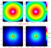 |
Fig. 5 Top panels: H2 column density distribution after 104 yr of constant mass loss for the model described in the text. The column density is integrated over all velocities. The right panel corresponds to a polar view of the CSE (line of sight perpendicular to the orbital plane) and the left panel to a view from the orbital plane. Bottom panels: H2 volume density in the plane of the sky for the same views. The figure corresponds to the last frame of a video showing the time growth of the CSE (online). |
3.3. Mass loss mechanism
As can be seen in Fig. 2, which shows the 12CO velocity-integrated emission profile at the declination of the star, the shell-intershell brightness contrast is >3 for r> 60′′, the radii where the shells seem resolved by the 30 m telescope beam. Decin et al. (2011) quote a typical value of 4 for the shell-intershell contrast of the FIR dust shells. The scattered light images of the inner region also suggest a similarly large contrast (3−5) (Mauron & Huggins 1999, 2000; Leao et al. 2006). Thus, on the scale of individual shells (the shell separation is typically 103 yr), the mass loss process is highly variable. Yet, as we have seen, it seems fairly stable averaged over longer timescales. Obviously, one must be looking for periodic events.
CW Leo is known to be a Mira-type variable. Mass loss is supposed to occur in Mira-type stars when the uppermost surface layers expand and become cool enough to form dust. Dust grains are accelerated outwards by the stellar radiation pressure, dragging gas on their way. However, the pulsation period of CW Leo, which is 649 days (Le Bertre 1982), is much too short to explain the spacing between the shells. Other periodic surface expansion events are linked to thermal pulses. Those result from the periodic ignition of the helium shell that surrounds the stellar carbon core. However, their period is much too long (few × 104 yr, Forestini & Charbonnel 1997). The time separation between the shells, 0.5 − 1 × 10³ yr, implies another mechanism.
The molecular shells of Fig. 1 are not exactly centred on CW Leo. This was first noticed by Guélin et al. (1993), who pointed out that the r = 15′′ shell visible on the v = 0 km s-1 CCH and C4H maps, despite its spherical shape, was centred 2′′ NW of the star. The authors suggested the shift results from an orbital motion of CW Leo. The motion, caused by the presence of a companion, would impart a drift velocity to the material expelled by the star. As a consequence, a shell of gas expelled near perihelion will drift away from the star in a direction that depends on the orbital phase at the time of its ejection. The ejection phase may vary from shell to shell leading to a complex rose-window like pattern similar to that of Fig. 3.
We have attempted to mimic the resulting pattern for a range of orbital parameters, using a simple model of the growth of an envelope around a binary system. Our model assumes that the mass loss rate of CW Leo is enhanced at certain phases of the orbital motion of the double star, e.g. near periastron in the case of a high excentricity orbit. The ejection mechanism, which may be linked to the change of the Roche lobe, is not considered by itself and the ejection of matter is assumed to be spherically symmetrical with respect to CW Leo. The ejected matter is a collection of shells consisting of freely moving particles, with an expansion velocity of 14.5 km s-1 with respect to CW Leo. The time step in our calculations is 2 yr. Consequently, each shell has a thickness of 9.15 × 1013 cm, i.e. 1.3 stellar radii. The gravitational wake of the companion, assumed to be lower in mass than CW Leo, is not considered. The particle motion is followed inside a grid attached to the centre of the double star system. A detailed description of the mathematical formalism can be found in He (2007). We have considered a number of cases by varying the total system mass Msys, the companion-to-CW Leo mass ratio (from 0.5 to 1.5), the orbital period (Po = 400 to 2000 yr), and the duration of the high mass loss episodes (Φ from 2π–0.5 to 0.5 rd). Figures 5 to 11 show different views of the matter (i.e. molecular gas) distribution in two cases of interest: constant mass loss and mass loss enhanced by a factor of 10 for a fraction of the orbit. In those examples, we assumed Msys = 3 M⊙; to ease the comparison, we choose in both cases the same orbit: circular with a radius of 130 AU, and a period P0 = 800 yr. The orbital velocity of CW Leo is 4.5 km s-1.
Figure 5 shows the patterns predicted after 104 yr of constant mass loss rate. The adopted gas density at r0 is 3 × 1010 cm-3. The figure shows a pattern of over-dense ring-like structures shaped by the orbital velocity transmitted by CW Leo to each expelled shell of matter. The mass and density distributions are symmetric with respect to the orbital plane. The polar view shows a tightly wrapped spiral pattern in the orbital plane. This type of spiral structure has been observed in the envelopes of AGB stars AFGL 3068 (Mauron & Huggins 2006) and, more recently, R Sculptoris (Maercker et al. 2012). Mastrodemos & Morris (1999), Kim & Tamm (2012), Kim et al. (2013), and He (2007) have computed several examples of such patterns. We note that the spirals appear in a natural way in binary star systems without the need of a discontinuous mass loss. The online video associated with Fig. 5 shows the spatial distribution of mater as a fonction of time, i.e. during the growth of the envelope, from t = 0 to 10 000 yr. Figure 6 allows us to compare the envelope for four different inclinations i of the orbital plane with respect to the line of sight. The spiral structure visible for i = 90° gets distorted when the inclination decreases. The edge-on view of the orbital plane shows two series of circles symmetrically shifted with respect to CW Leo. To obtain a better insight and constrain the orbit inclination, we have computed the column density of gas, N(H2), for velocities from −14.5 km s-1 to 14.5 km s-1. Figure 7 shows N(H2) for V − V∗ = 0 km s-1 and the associated online video N(H2) for all velocities.
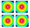 |
Fig. 6 H2 column density distribution, in units of 1021 cm-2, at t = 10 000 yr for the same model as in Fig. 5, but for different inclinations of the line of sight with respect to the orbital plane. |
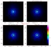 |
Fig. 7 H2 distribution of the gas at the velocity of the star at t = 10 000 yr. The model parameters are the same as in Fig. 5. The figure corresponds to the middle frame of a video showing the distribution of matter in the envelope at different velocities (online). |
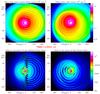 |
Fig. 8 Top panels: H2 column density distribution after 104 yr derived for the case of a periodic mass loss enhancement caused by the close fly-by of a companion star with an orbital period of 800 yr for the model described in the text. The column density is integrated over all velocities. The right panel corresponds to a polar view of the CSE (line of sight perpendicular to the orbital plane) and the left panel to a view from the orbital plane. Bottom panels: H2 volume density in the plane of the sky for the same views. The figure corresponds to the last frame of a video showing the time growth of the CSE (online). |
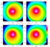 |
Fig. 9 Total H2 column density (in units of 1021 cm-2) after 10 000 yr, for the same model as Fig. 8 at different inclinations of the line of view with respect to the orbital plane. |
Figure 8 shows the pattern produced by periodic mass loss enhancements. The parameters are the same as in Fig. 5. The orbital parameters are chosen to be the same as in Figs. 5 through 7 to make the comparison with Fig. 5 more pertinent. The mass loss integrated over one period is the same as in Fig. 5, but the mass loss rate increases by a factor of 10 when the orbital phase is within 30° from phase 0 (i.e. periastron for an elliptical orbit).
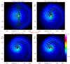 |
Fig. 10 Spatial distribution of matter at t = 10 000 yr for a velocity of the gas with respect to the star of 0 km -1 in the case of periodic mass loss (same parameters as in Fig. 8). The figure corresponds to the middle frame of a video showing the distribution of matter in the envelope at different velocities (online). |
Figure 8, i.e. the periodic mass loss simulation, replicates several key features of Fig. 1: i) the presence of a number of over-dense rings in the plane of the sky (see the polar view: lower right figure), some of which intersect at places; ii) increasing separation between the bright rings at large radii; and iii) asymmetrical envelope extent in the orbital plane. Figure 9 shows the total N(H2) at t = 10 000 yr for different inclinations of the orbital plane, and Fig. 10 and its associated online video, N(H2) as a function of the gas velocity. The CO line profiles in IRC+10216, like those of most molecular lines (Cernicharo et al. 2000), show a range of velocities restricted to V − V∗ = −14.5 to 14.5 km s-1, with very sharp edges. This is consistent with a near face-on orientation of the orbital plane: a much smaller inclination of the plane to the line of sight would produce a significant line broadening in the form of line wings because of the change in the star apparent radial velocity between the mass loss events.
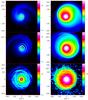 |
Fig. 11 Gas distribution at t = 10 000 yr for an enhanced mass loss with periods of 400 yr (upper panels) and 800 yr (middle panels), compared to the observed CO(2−1) line brightness distribution (lower panel). The model data have been convolved with a Gaussian of width equal to the telescope HPBW. The left panels show the distribution of the gas for velocities (V − V∗) = ± 2 km s-1 and the right panels the gas column density integrated over all velocities. |
Figure 11 shows a comparison between the episodic mass loss model of Fig. 8 and the observations. The model data have been convolved with a Gaussian of width equal to the telescope HPBW, i.e. 11′′. The left panels show the distribution of the gas for velocities (V − V∗) = ± 2 km s-1. The right panels show the gas column density integrated over all velocities. The upper panels correspond to the episodic mass loss model shown in Fig. 8, with an orbital period of 400 yr (top panels) and 800 years (middle panels). The bottom panels show the observed 12CO (2−1) brightness distributions. Obviously, the actual gas distribution is more complex than simulated by our simple model, but the longer period of 800 years yields images much more similar to those observed. The shell-intershell density contrast appears more clearly on the narrow velocity maps (left panels).
The most likely model, according to our simulations, is that of a strongly enhanced mass-loss rate triggered every ≃800 yr by the fly-by of a ≃1 M⊙ companion (the mass of CW Leo is believed to be ≃2 M⊙, Guélin et al. 1997) on an orbit almost perpendicular to the light of sight. The orbit is probably excentric and the high mass-loss episodes probably occur near periastron; they last long enough for CW Leo to change its orbital velocity by 1−2 rd so that the outer envelope appears asymmetric.
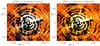 |
Fig. 12 Contour levels of the CO(2−1) line intensity superimposed on the PSF-deconvolved, halo-subtracted 100 μm map of PACS (Fig. 2 of Decin et al. 2011). (Left: CO in the velocity interval (V − V∗) = ± 2 km s-1; right CO integrated over all velocities). Light blue contours levels: 1 to 6 K by steps of 1 K, yellow contours: 10 to 70 K km s-1 by 1 K km s-1. The dark blue contour levels represent 0.9 times the adjacent light blue contour levels and the green contours 0.85 times the adjacent yellow contours. |
In this respect, it is instructive to compare both the simulated maps and the observed CO maps with the map of the dust FIR emission reported by Decin et al. (2011). This is done in Fig. 12, where we superimpose on the PSF-deconvolved and halo-subtracted PACS map (Fig. 2 of Decin et al. 2011) the intensity contour levels of our 12CO(2−1) maps (lower panels of Fig. 11). Both the integrated-velocity CO contour levels and the CO contours with (V − V∗) = ±2 km s-1 are shown. Because dust and gas should be coeval and because the dust emission is optically thin at 100 μm, dust emission should be preferably compared to the integrated-velocity CO map. Several bright FIR arc-like features appear to closely follow the bright rims of the CO shells (e.g. the rim 110′′ N from the star, the rims 50′′ and 100′′ SW from the star), albeit some dark FIR areas also fall atop bright CO rims (e.g. at 90′′ W from the star). Although artefacts caused by the PACS PSF deconvolution make the comparison difficult, an overall correlation of the CO and FIR dust emissions seems clear.
Observations of the CO(2−1) emission, at a much higher resolution, are in progress with the SMA, the PdB Interferometer, and for the inner envelope, ALMA. The CO shells, viewed with an angular resolution of 3′′ or higher appear thinner and more clumpy than in Fig. 1. These differences make it ineffectual to try to simulate the pattern of Fig. 1, which is affected by beam smearing, more precisely. A definitive assessment the binary scenario must await completion of the interferometer maps.
After the submission of this article, we learned about the publication of a first ALMA study of the close surroundings (r< 3′′) of CW Leo (Decin et al. 2015), and the discovery of a faint point-like object near CW Leo that could be a companion star (Kim et al. 2014). The 13CO (6−5) emission is resolved by ALMA into a central source plus a couple of arc-like features at ≃2′′ from CW Leo. Those are interpreted as part of a spiral structure induced by a companion star. The period (55 years) and orbit (diameter 20−25 AU, seen edge-on) of such a companion are however quite different from those of our model and would be difficult to reconcile with our outer envelope observations, in particular with the cusped molecular line shapes and the spherical 3D shape of the observed shells. The small field of view of the ALMA observations and lack of short spacings (which causes a negative lobes in the maps) preclude following the arc-like features at radii larger or smaller than 2′′, making the identification of a spiral very tentative for the time being. The arc-like features, on the other hand, could be pieces of a new shell, ejected some 80 yr ago when our model companion was near periastron.
The point-like object, discovered by Kim et al. (2014) on 2011 HST images, is interpreted by these authors as a possible companion M star. Its apparent distance from CW Leo (0.5′′, or 65 AU) is compatible with that of our model companion.
4. Conclusion
Our 12CO(2−1) and 13CO(2−1) line emission maps of IRC+10216, made with the IRAM 30 m telescope, reveal the presence of over-dense spherical shells, some of which have already been noticed on optical images or in the dust thermal emission. The CO emission peaks on the central star, CW Leo, but remains relatively strong up to r = 180′′ from that star. Its intensity drops or vanishes further out. We interpret the sudden decrease of the CO brightness to photodissociation and set the photodissociation limit rphot to that radius.
The CO envelope fits well inside the large bow-shock discovered by Sahai & Chronopoulos (2010) and must be freely expanding into the cavity cleared up by the shock. Outside the tiny (<1′′) dust formation region where the expelled matter is accelerated, the gas expands radially at a remarkably constant velocity: 14.5 km s-1. For a distance of 130 pc, the photodissociation radius corresponds to a look-back time of ≃8000 yr. Because of CO self-shielding, CO should be a reliable tracer of the molecular gas up to rphot, and the 12CO(2−1) and 13CO(2−1) maps must teach us about the mass loss history in that period of time.
The over-dense shells show that the mass loss process is highly variable on timescales of hundreds of years. Previous studies suggested that the average mass loss rate has strongly decreased in the last few thousand years. Comparing the intensities of the CO lines near the star, across the envelope and beyond rphot we do not see evidence of such a decrease: the mass-loss rate averaged over periods of 103 yr appears to be 2 − 4 × 10⁻⁵ M⊙ yr-1 and to stay constant within a factor of 2, which is about the accuracy attached to our mass derivation method.
The velocity-channel 12CO(2−1) emission maps, particularly the map at the star velocity that traces the molecular gas in the plane of the sky, show a succession of bright circles that denote the rims of the over-dense shells. The circles are not concentric as one may expect in the case of a spherical outflow, but shifted by several arcsec in different directions; the outermost shells extend farther to the N-NE. The typical shell separation is 800 − 1000 yr and seems to increase outwards. The shell-intershell brightness contrast is ≥3 in the outer envelope.
These key features can all be accounted for if CW Leo has a companion star with an excentric orbit and if the mass loss increases when the companion is close to periastron. Another mass loss mechanism that has been proposed is a cyclic magnetic activity at the stellar surface, similar to that on the Sun (Soker 2000). Mira-type oscillations and thermal pulses seem to be ruled out because their periods are much shorter or longer than implied by the shell separation. The angular resolution of the CO observations reported here does allow us to not properly resolve the shells and their substructures. Higher angular resolution observations are currently in progress at the SMA, PdBI, and ALMA. Hopefully, they will enable us to decide on the mass ejection mechanism and yield more reliable values of the mass-loss rate and of the shell-intershell density contrast. The latter is of great importance for a better understanding of circumstellar chemistry (see e.g. Guélin et al. 1999; Cordiner & Millar 2009).
Online material
Movie of Fig. 3 Access Supplementary Material
Movie of Fig. 5 Access Supplementary Material
Movie of Fig. 7 Access Supplementary Material
Movie of Fig. 8 Access Supplementary Material
Movie of Fig. 10 Access Supplementary Material
We adopt a distance to CW Leo of 130 pc (Agúndez et al. 2012) and assume a uniform expansion velocity of 14.5 km s-1 (Cernicharo et al. 2000).
Acknowledgments
We thank Spanish MICINN for funding support through grants AYA2006-14876, AYA2009-07304, and the CONSOLIDER program “ASTROMOL” CSD2009-00038. The research leading to these results has received funding from the European Research Council under the European Union’s Seventh Framework Programme (FP/2007−2013)/ERC-2013-SyG, Grant Agreement No. 610256 NANOCOSMOS. M.G. acknowledges support from the CNRS program PCMI, as well as from the SMA.
References
- Agúndez, M., & Cernicharo, J. 2006, ApJ, 650, 393 [Google Scholar]
- Agúndez, M., Cernicharo, J., Guélin, M., et al. 2010, A&A, 517, L2 [NASA ADS] [CrossRef] [EDP Sciences] [Google Scholar]
- Agúndez, M., Fonfría, J. P., Cernicharo, J., et al. 2012, A&A, 543, A48 [NASA ADS] [CrossRef] [EDP Sciences] [Google Scholar]
- Balick, B., & Frank, A. 2002, ARA&A, 40, 439 [NASA ADS] [CrossRef] [Google Scholar]
- Cabezas, C., Cernicharo, J., Alonso, J. L., et al. 2013, ApJ, 775, 133 [NASA ADS] [CrossRef] [Google Scholar]
- Cernicharo, J. 1985, ATM a code to compute atmospheric opacity up to 1 THz, IRAM internal report [Google Scholar]
- Cernicharo, J. 2004, ApJ, 608, L41 [NASA ADS] [CrossRef] [Google Scholar]
- Cernicharo, J. 2012, in ECLA-2011: Proc. of the European Conference on Laboratory Astrophysics, eds. C. Stehl, C. Joblin, & L. d’Hendecourt (Cambridge: Cambridge Univ. Press), EAS Pub. Ser., 251 [Google Scholar]
- Cernicharo, J., & Guélin, M. 1987, A&A, 183, L10 [NASA ADS] [Google Scholar]
- Cernicharo, J., & Guélin, M. 1996, A&A, 309, L27 [NASA ADS] [Google Scholar]
- Cernicharo, J., Guélin, M., Kahane, C., et al. 1991, A&A, 246, 213 [NASA ADS] [Google Scholar]
- Cernicharo, J., Barlow, M., González, E., et al. 1996, A&A, 315, L201 [NASA ADS] [Google Scholar]
- Cernicharo, J., Guélin, M., & Kahane, C. 2000, A&AS, 142, 181 [NASA ADS] [CrossRef] [EDP Sciences] [Google Scholar]
- Cernicharo, J., Guélin, M., Agúndez, M., et al. 2008, ApJ, 688, L83 [NASA ADS] [CrossRef] [Google Scholar]
- Cernicharo, J., Waters, L. B. F. M., Decin, L., et al. 2010, A&A, 521, L8 [NASA ADS] [CrossRef] [EDP Sciences] [Google Scholar]
- Cernicharo, J., Teyssier, D., Quintana, G., et al. 2014, ApJ, 796, L21 [NASA ADS] [CrossRef] [Google Scholar]
- Cordiner, M. A., & Millar, T. J. 2009, ApJ, 697, 68 [NASA ADS] [CrossRef] [Google Scholar]
- Crabtree, D. R., McLaren, R. A., & Christian, C. A. 1987, in Late Stages of Stellar Evolution, eds. S. Kwok, & S. R. Pottasch (Reidel Publishing Company), 145 [Google Scholar]
- Crosas, M., & Menten, K. M. 1997, ApJ, 483, 913 [NASA ADS] [CrossRef] [Google Scholar]
- De Beck, E., Lombaert, R., Agúndez, M., et al. 2012, A&A, 539, A108 [NASA ADS] [CrossRef] [EDP Sciences] [Google Scholar]
- Decin, L., Royer, P., Cox, N. L. J., et al. 2011, A&A, 534, A1 [NASA ADS] [CrossRef] [EDP Sciences] [Google Scholar]
- Decin, L., Richards, A. M. S., Neufeld, D., et al. 2015, A&A, 574, A5 [NASA ADS] [CrossRef] [EDP Sciences] [Google Scholar]
- Doty, F. P., & Leung, C. M. 1998, ApJ, 502, 898 [NASA ADS] [CrossRef] [Google Scholar]
- Fazio, G. G., Stier, M. T., Wright, E. L., & McBreen, B. 1980, ApJ, 237, L39 [NASA ADS] [CrossRef] [Google Scholar]
- Fonfría, J. P., Cernicharo, J., Richter, M. J., & Lacy, J. H. 2008, ApJ, 673, 445 [NASA ADS] [CrossRef] [Google Scholar]
- Fong, D., Meixner, M., & Shah, R. Y. 2003, ApJ, 582, L39 [NASA ADS] [CrossRef] [Google Scholar]
- Ford, K. E. S., Neufeld, D. A., Goldsmith, P. F., & Melnick, G. J. 2003, ApJ, 589, 430 [NASA ADS] [CrossRef] [Google Scholar]
- Ford, K. E. S., Neufeld, D. A., Schilke, P., & Melnick, G. J. 2004, ApJ, 614, 990 [NASA ADS] [CrossRef] [Google Scholar]
- Forestini, M., & Charbonnel, C. 1997, A&AS, 123, 241 [NASA ADS] [CrossRef] [EDP Sciences] [Google Scholar]
- Gehrz, R. 1989, in Interstellar Dust, Proc. 135th Symp. IAU, eds. L. J. Allamandola, & A. G. G. M. Tielens (Dordrecht: Kluwer Academic Publishers), 445 [Google Scholar]
- Greve, A., Kramer, C., & Wild, W. 2012, A&AS, 133, 271 [Google Scholar]
- Groenewegen, M. A. T. 1997, A&A, 317, 503 [NASA ADS] [Google Scholar]
- Groenewegen, M. A. T., van der Veen, W. E. C. J., & Matthews, H. E. 1998, A&A, 338, 491 [NASA ADS] [Google Scholar]
- Guélin, M., Lucas, R., & Cernicharo, J. 1993, A&A, 280, L19 [NASA ADS] [Google Scholar]
- Guélin, M., Cernicharo, J., Travers, M. J., et al. 1997, A&A, 317, L1 [NASA ADS] [Google Scholar]
- Guélin, M., Neininger, N., Lucas, R., & Cernicharo, J. 1999, in The Physics and Chemistry of the Interstellar Medium, eds. V. Ossenkopf, et al. (Herdecke: GCA-Verlag), 236 [Google Scholar]
- Haniff, C. A., & Buscher, D. F. 1998, A&A, 334, L5 [NASA ADS] [Google Scholar]
- He, J. H. 2007, A&A, 467, 1081 [NASA ADS] [CrossRef] [EDP Sciences] [Google Scholar]
- Herbig, G. H., & Zappala, R. R. 1970, ApJ, 162, L15 [NASA ADS] [CrossRef] [Google Scholar]
- Jura, M. 1974, ApJ, 191, 375 [NASA ADS] [CrossRef] [Google Scholar]
- Kahane, C., Gómez-Gónzalez, J., Cernicharo, J., & Guélin, M. 1988, A&A, 190, 167 [NASA ADS] [Google Scholar]
- Kastner, J. H., & Weintraub, D. A. 1994, ApJ, 434, 719 [NASA ADS] [CrossRef] [Google Scholar]
- Kim, H., & Taam, R. E. 2012, ApJ, 759, 59 [NASA ADS] [CrossRef] [Google Scholar]
- Kim, H., Hsieh, I.-Ta, Lieu, S.-Y., & Taam, R. E. 2013, ApJ, 776, 86 [NASA ADS] [CrossRef] [Google Scholar]
- Kim, H., Lee, H.-G., & Mauron, N. 2014 [arXiv:1412.0083] [Google Scholar]
- Kramer, C., Peñalver, J., & Greve, A. 2013, Improvement of the IRAM 30 m telescope beam pattern, IRAM internal report [Google Scholar]
- Leao, I. C., de Laverny, P., Mékarnia, D., et al. 2006, A&A, 455, 187 [NASA ADS] [CrossRef] [EDP Sciences] [Google Scholar]
- Le Bertre, T. 1982, A&AS, 94, 377 [Google Scholar]
- Lucas, R., Guélin, M., Kahane, C., et al. 1995, Ap&SS, 224, 293 [NASA ADS] [CrossRef] [Google Scholar]
- Maercker, M., Mohamed, S., Vlemmings, W. H. T., et al. 2012, Nature, 490, 232 [NASA ADS] [CrossRef] [PubMed] [Google Scholar]
- Mamon, G. A., Glassgold, A. E., & Huggins, P. J. 1998, ApJ, 328, 797 [Google Scholar]
- Mastrodemos, N., & Morris, M. 1999, ApJ, 523, 357 [NASA ADS] [CrossRef] [Google Scholar]
- Mauron, N., & Huggins, P. J. 1999, A&A, 349, 203 [NASA ADS] [Google Scholar]
- Mauron, N., & Huggins, P. J. 2000, A&A, 359, 707 [NASA ADS] [Google Scholar]
- Mauron, N., & Huggins, P. J. 2006, A&A, 452, 257 [NASA ADS] [CrossRef] [EDP Sciences] [Google Scholar]
- McCarthy, M. C., Gottlieb, C. A., Gupta, H., & Thaddeus, P. 2006, ApJ, 652, L141 [NASA ADS] [CrossRef] [Google Scholar]
- Melnick, G. J., Neufeld, D. A., Ford, K. E. S., et al. 2001, Nature, 412, 160 [NASA ADS] [CrossRef] [PubMed] [Google Scholar]
- Men’shchikov, A. B., Balega, Y., Blöcker, T., Osterbart, R., & Weigelt, G. 2001, A&A, 368, 497 [NASA ADS] [CrossRef] [EDP Sciences] [Google Scholar]
- Monnier, J. D., Danchi, W. C., Hale, D. S., et al. 2000, ApJ, 543, 861 [Google Scholar]
- Morris, M., & Jura, M. 1983, ApJ, 267, 179 [NASA ADS] [CrossRef] [Google Scholar]
- Nollett, K. M., Busso, M., & Wasserburg, G. J. 2003, ApJ, 582, 1036 [Google Scholar]
- Ohishi, M., Kaifu, N., Kawaguchi, K., et al. 1989, ApJ, 345, L83 [NASA ADS] [CrossRef] [Google Scholar]
- Pardo, J. R., & Cernicharo, J. 2007, ApJ, 654, 978 [NASA ADS] [CrossRef] [Google Scholar]
- Pardo, J. R., Cernicharo, J., & Serabyn, E. 2001, IEEE Trans. Antennas and Propagation, 49, 1683 [Google Scholar]
- Sahai, R., & Chronopoulos, C. K. 2010, ApJ, 711, L53 [NASA ADS] [CrossRef] [Google Scholar]
- Schöier, F. L., & Olofsson, H. 2000, A&A, 359, 586 [NASA ADS] [Google Scholar]
- Schöier, F. L., & Olofsson, H. 2001, A&A, 368, 969 [NASA ADS] [CrossRef] [EDP Sciences] [Google Scholar]
- Schuster, K. F., Boucher, C., Brunswig, W., et al. 2004, A&A, 423, 1171 [NASA ADS] [CrossRef] [EDP Sciences] [Google Scholar]
- Skinner, C. J., Meixner, M., & Bobrowsly, M. 1998, MNRAS, 300, L29 [NASA ADS] [CrossRef] [Google Scholar]
- Soker, N. 2000, ApJ, 540, 436 [NASA ADS] [CrossRef] [Google Scholar]
- Solomon, P. M., Jefferts, K. B., Penzias, A. A., & Wilson, R. W. 1971, ApJ, 163, L53 [NASA ADS] [CrossRef] [Google Scholar]
- Stanek, K. Z., Knapp, G. R., Young, K., & Phillips, T. G. 1995, ApJS, 100, 169 [NASA ADS] [CrossRef] [Google Scholar]
- Teyssier, D., Hernandez, R., Bujarrabal, V., et al. 2006, A&A, 450, 167 [NASA ADS] [CrossRef] [EDP Sciences] [Google Scholar]
- Thaddeus, P., Cummins, S. E., & Linke, R. A. 1984, ApJ, 283, L45 [NASA ADS] [CrossRef] [Google Scholar]
- Thaddeus, P., Gottlieb, C. A., Gupta, H., et al. 2008, ApJ, 677, 1132 [NASA ADS] [CrossRef] [Google Scholar]
- Trung, D. V., & Lim, J. 2008, ApJ, 678, 303 [NASA ADS] [CrossRef] [Google Scholar]
- Tuthill, P. G., Monnier, J. D., Danchi, W. C., & Lopez, B. 2000, ApJ, 543, 284 [NASA ADS] [CrossRef] [Google Scholar]
- Vlemmings, W. H. T., Maercker, M., Lindqvist, M., et al. 2013, A&A, 556, L1 [NASA ADS] [CrossRef] [EDP Sciences] [Google Scholar]
All Figures
|
Fig. 1 Top left box: velocity-integrated CO (J = 2−1) line emission in the central 400′′ × 400′′ area (VLSR range from −41 to −12 km s-1). Other upper maps: velocity-channel maps (resolution 2 km s-1); marked velocities are relative to the LSR systemic star velocity (V∗ = −26.5 km s-1); the units of the color scale correspond to K km s-1. Positive and negative velocities correspond to the rear and front parts of the envelope, respectively. Bottom right panels: observed 12CO(2−1) line profiles along a strip to the east for Δδ = 0′′; the upper left numbers indicate Δα in arcseconds and the upper right numbers the intensity scaling factor applied to plot all spectra at the same |
| In the text | |
|
Fig. 2 Black line: intensity of the 12CO(2−1) line integrated between LSR velocities −25.5 and −27.5 km s-1 observed along an EW strip at the declination of the star (Δδ = 0′′). Red line: the response of the telescope error beam to the 12CO(2−1) emission along the same strip. The error beam consists of 3 Gaussians of full width at half power (FWHP) 65′′, 250′′, and 860′′ and intensities 1.9 × 10⁻³, 3.5 × 10⁻⁴, and 2.2 × 10⁻⁵ relative to the main beam, respectively. Blue line: the 12CO(2−1) line intensity after removal of the error beam response. |
| In the text | |
|
Fig. 3 Main beam-averaged 12CO(2−1) line brightness temperature observed at VLSR − V∗ = 0 km s-1 (Δv = 0.1 km s-1). This is the central frame of a video showing the distribution of the 12CO line emission at different velocities (online). |
| In the text | |
|
Fig. 4 Left panel: 13CO J = 1 − 0 and J = 2−1 line profiles (black and red histograms, respectively), averaged over concentric rings of width Δr = 10′′, observed at radii ranging from r = 0′′ to 130′′. The ordinate scale (black numbers) applies to the J = 1 − 0 line profile (black). The number in red in the upper left corner is the factor by which the J = 2−1 profile (red) has been divided to match the intensity scale. For r< 90′′ it also represents the R21 = 13CO(2−1)/13CO(1−0) velocity-integrated line intensity ratio. Right panel: J = 2−112CO (black) and 13CO line profiles averaged over the same 10′′-wide rings. The ordinate scale applies to the 13CO(2−1) line profile (red). The number in black in the upper left corner is the factor by which the 12CO(2−1) profile (black) has been divided to match the intensity scale. For r ≥ 40′′, it also represents the Ri = 12CO(2−1)/13CO(2−1) velocity-integrated line intensity ratio. |
| In the text | |
|
Fig. 5 Top panels: H2 column density distribution after 104 yr of constant mass loss for the model described in the text. The column density is integrated over all velocities. The right panel corresponds to a polar view of the CSE (line of sight perpendicular to the orbital plane) and the left panel to a view from the orbital plane. Bottom panels: H2 volume density in the plane of the sky for the same views. The figure corresponds to the last frame of a video showing the time growth of the CSE (online). |
| In the text | |
|
Fig. 6 H2 column density distribution, in units of 1021 cm-2, at t = 10 000 yr for the same model as in Fig. 5, but for different inclinations of the line of sight with respect to the orbital plane. |
| In the text | |
|
Fig. 7 H2 distribution of the gas at the velocity of the star at t = 10 000 yr. The model parameters are the same as in Fig. 5. The figure corresponds to the middle frame of a video showing the distribution of matter in the envelope at different velocities (online). |
| In the text | |
|
Fig. 8 Top panels: H2 column density distribution after 104 yr derived for the case of a periodic mass loss enhancement caused by the close fly-by of a companion star with an orbital period of 800 yr for the model described in the text. The column density is integrated over all velocities. The right panel corresponds to a polar view of the CSE (line of sight perpendicular to the orbital plane) and the left panel to a view from the orbital plane. Bottom panels: H2 volume density in the plane of the sky for the same views. The figure corresponds to the last frame of a video showing the time growth of the CSE (online). |
| In the text | |
|
Fig. 9 Total H2 column density (in units of 1021 cm-2) after 10 000 yr, for the same model as Fig. 8 at different inclinations of the line of view with respect to the orbital plane. |
| In the text | |
|
Fig. 10 Spatial distribution of matter at t = 10 000 yr for a velocity of the gas with respect to the star of 0 km -1 in the case of periodic mass loss (same parameters as in Fig. 8). The figure corresponds to the middle frame of a video showing the distribution of matter in the envelope at different velocities (online). |
| In the text | |
|
Fig. 11 Gas distribution at t = 10 000 yr for an enhanced mass loss with periods of 400 yr (upper panels) and 800 yr (middle panels), compared to the observed CO(2−1) line brightness distribution (lower panel). The model data have been convolved with a Gaussian of width equal to the telescope HPBW. The left panels show the distribution of the gas for velocities (V − V∗) = ± 2 km s-1 and the right panels the gas column density integrated over all velocities. |
| In the text | |
|
Fig. 12 Contour levels of the CO(2−1) line intensity superimposed on the PSF-deconvolved, halo-subtracted 100 μm map of PACS (Fig. 2 of Decin et al. 2011). (Left: CO in the velocity interval (V − V∗) = ± 2 km s-1; right CO integrated over all velocities). Light blue contours levels: 1 to 6 K by steps of 1 K, yellow contours: 10 to 70 K km s-1 by 1 K km s-1. The dark blue contour levels represent 0.9 times the adjacent light blue contour levels and the green contours 0.85 times the adjacent yellow contours. |
| In the text | |
Current usage metrics show cumulative count of Article Views (full-text article views including HTML views, PDF and ePub downloads, according to the available data) and Abstracts Views on Vision4Press platform.
Data correspond to usage on the plateform after 2015. The current usage metrics is available 48-96 hours after online publication and is updated daily on week days.
Initial download of the metrics may take a while.