| Issue |
A&A
Volume 575, March 2015
|
|
|---|---|---|
| Article Number | A4 | |
| Number of page(s) | 17 | |
| Section | Stellar atmospheres | |
| DOI | https://doi.org/10.1051/0004-6361/201424409 | |
| Published online | 10 February 2015 | |
The Gaia-ESO Survey: Chromospheric emission, accretion properties, and rotation in γ Velorum and Chamaeleon I⋆,⋆⋆,⋆⋆⋆
1 INAF–Osservatorio Astrofisico di Catania, via S. Sofia 78, 95123 Catania, Italy
e-mail: This email address is being protected from spambots. You need JavaScript enabled to view it.
2 Dipartimento di Fisica e Astronomia, Sezione Astrofisica, Università di Catania, via S. Sofia 78, 95123 Catania, Italy
3 INAF–Osservatorio Astronomico di Capodimonte, via Moiariello 16, 80131 Naples, Italy
4 INAF–Osservatorio Astronomico di Palermo, Piazza del Parlamento 1, 90134 Palermo, Italy
5 INAF–Osservatorio Astrofisico di Arcetri, Largo E. Fermi 5, 50125 Firenze, Italy
6 Astrophysics Group, Keele University, Keele, Staffordshire ST5 5BG, UK
7 Departamento de Astrofísica y Ciencias de la Atmósfera, Universidad Complutense de Madrid, 28040 Madrid, Spain
8 Instituto de Astrofísica de Andalucía, CSIC, Apdo 3004, 18080 Granada, Spain
9 School of Physics, Astronomy & Mathematics, University of Hertfordshire, College Lane, Hatfield, Hertfordshire, AL10 9AB, UK
10 Dipartimento di Fisica e Chimica, Università di Palermo, Piazza del Parlamento 1, 90134 Palermo, Italy
11 Centro de Astrofísica, Universidade do Porto, Rua das Estrelas, 4150-752 Porto, Portugal
12 S. D. Astronomía y Geodesia, Facultad de Ciencias Matemáticas, Universidad Complutense de Madrid, 28040 Madrid, Spain
13 European Southern Observatory, Karl-Schwartzschild-Strasse 2, 85748 Garching bei München, Germany
14 Departamento de Física e Astronomia, Faculdade de Ciências, Universidade do Porto, Rua do Campo Alegre, 4169-007 Porto, Portugal
15 Institute of Astronomy, University of Cambridge, Madingley Road, Cambridge CB3 0HA, UK
16 INAF–Osservatorio Astronomico di Bologna, via Ranzani 1, 40127 Bologna, Italy
17 Max-Planck Institut für Astronomie, Königstuhl 17, 69117 Heidelberg, Germany
18 Instituto de Física y Astronomía, Facultad de Ciencias, Universidad de Valparaíso, Av. Gran Bretaña 1111, Playa Ancha, Valparaíso, Chile
19 Laboratoire Lagrange (UMR 7293), Université de Nice Sophia Antipolis, CNRS, Observatoire de la Côte d’Azur, CS 34229, 06304 Nice Cedex 4, France
Received: 16 June 2014
Accepted: 8 December 2014
Abstract
Aims. One of the goals of the Gaia-ESO Survey (GES), which is conducted with FLAMES at the VLT, is the census and the characterization of the low-mass members of very young clusters and associations. We conduct a comparative study of the main properties of the sources belonging to γ Velorum (γ Vel) and Chamaeleon I (Cha I) young associations, focusing on their rotation, chromospheric radiative losses, and accretion.
Methods. We used the fundamental parameters (effective temperature, surface gravity, lithium abundance, and radial velocity) delivered by the GES consortium in the first internal data release to select the members of γ Vel and Cha I among the UVES and GIRAFFE spectroscopic observations. A total of 140 γ Vel members and 74 Cha I members were studied. The procedure adopted by the GES to derive stellar fundamental parameters also provided measures of the projected rotational velocity (vsini). We calculated stellar luminosities through spectral energy distributions, while stellar masses were derived by comparison with evolutionary tracks. The spectral subtraction of low-activity and slowly rotating templates, which are rotationally broadened to match the vsini of the targets, enabled us to measure the equivalent widths (EWs) and the fluxes in the Hα and Hβ lines. The Hα line was also used for identifying accreting objects, on the basis of its EW and the width at the 10% of the line peak (10%W), and for evaluating the mass accretion rate (Ṁacc).
Results. The distribution of vsini for the members of γ Vel displays a peak at about 10 km s-1 with a tail toward faster rotators. There is also some indication of a different vsini distribution for the members of its two kinematical populations. Most of these stars have Hα fluxes corresponding to a saturated activity regime. We find a similar distribution, but with a narrower peak, for Cha I. Only a handful of stars in γ Vel display signatures of accretion, while many more accretors were detected in the younger Cha I, where the highest Hα fluxes are mostly due to accretion, rather than to chromospheric activity. Accreting and active stars occupy two different regions in a Teff–flux diagram and we propose a criterion for distinguishing them. We derive Ṁacc in the ranges 10-11–10-9 M⊙ yr-1 and 10-10–10-7 M⊙ yr-1 for γ Vel and Cha I accretors, respectively. We find less scatter in the Ṁacc − M⋆ relation derived through the Hα EWs, when compared to the Hα10%W diagnostics, in agreement with other authors.
Key words: stars: chromospheres / stars: low-mass / open clusters and associations: individual:γVelorum / stars: rotation / open clusters and associations: individual: Chamaeleon I / stars: pre-main sequence
Based on data products from observations made with ESO Telescopes at the La Silla Paranal Observatory under programme ID 188.B-3002.
Tables 5, 6, and Appendix A are available in electronic form at http://www.aanda.org
Tables 2–4 are only available at the CDS via anonymous ftp to cdsarc.u-strasbg.fr (130.79.128.5) or via http://cdsarc.u-strasbg.fr/viz-bin/qcat?J/A+A/575/A4
© ESO, 2015
1. Introduction
During the pre-main sequence (PMS) evolutionary phase, solar-like and low-mass stars undergo remarkable changes of their internal structure, radius, temperature and rotation velocity. Moreover, several phenomena affect their atmospheric layers and circumstellar environments with noticeable effects on the observed spectra.
The rotation velocity distribution of stars in young clusters and associations is a fundamental tool for understanding the relative importance of the processes that lead the stars to spin up during their early life (contraction and mass accretion) over those that tend to slow down them (magnetic braking and disk locking). Disks appear to regulate the stellar rotation only for about the first 5 Myr of their life or less, when they are very frequent and detected at infrared wavelengths (e.g., Lada et al. 2006; Sicilia-Aguilar et al. 2006, and references therein) and accretion signatures, such as strong and broad emission lines, are seen in the stellar spectra. After 5 Myr the disks dissipate quickly (e.g., Haisch et al. 2001; Hernández et al. 2008) and the stars are free to spin up as they contract and approach the zero-age main-sequence (ZAMS). The disk-locking effect has been invoked as responsible for the bimodal distribution of rotation periods observed in very young clusters for stars with M> 0.25 M⊙ with the slower rotators being very often objects with infrared excess from circumstellar disks (e.g., Herbst et al. 2002; Rebull et al. 2002). The presence of both slow and fast rotators is still observed in older clusters and associations with ages from about 30 to 200 Myr (see, e.g., Messina et al. 2003, 2010; Meibom et al. 2009, and references therein) and predicted by the models of angular momentum evolution (e.g., Bouvier et al. 1997; Spada et al. 2011).
The magnetic activity is closely related to the stellar evolution during the PMS and main-sequence (MS) stages, and the resulting changes in the internal structure and surface rotation rate. Indeed, the dynamo mechanism generating the magnetic fields depends on the stellar rotation, differential rotation, and subphotospheric convection. For stars in the MS phase, the level of magnetic activity, as expressed by the average chromospheric emission (CE), has been shown to decay with age owing to magnetic braking, since the pioneering work of Skumanich (1972), who proposed a simple power law of the form CE ∝ t− 1/2. Other works based on stars belonging to clusters and moving groups of different ages have proposed different relations between CE and age (see, e.g., Soderblom et al. 1991; Pace & Pasquini 2004; Mamajek & Hillenbrabd 2008). Recent indications support the CE decline with age until about 2 Gyr and nearly constant behavior thereafter (e.g., Pace 2013). The age-activity-rotation relation has been also investigated by means of the X-ray coronal emission (e.g., Pizzolato et al. 2003; Preibisch & Feigelson 2005). However, their faintness has meant that very low-mass stars in many open clusters (OCs) and associations have only recently been observed.
The picture is more complicated for stars in the PMS phase, when accretion of material from the circumstellar disk onto the central star occurs. In particular, mass accretion in the early PMS evolution is responsible for a significant fraction of the final stellar mass and the time dependence of the mass accretion rate is important for tracing the disk evolution and its dissipation, contributing to the conditions for both stellar and planetary formation (e.g., Hartmann 1998). This implies that, during the PMS evolutionary phases, mass accretion affects the spectral diagnostics of CE, and, at the same time, chromospheric activity can be a source of contamination in the measurements of mass accretion rates. The effects of accretion and magnetic activity on the optical emission lines become comparable at the final stages of the PMS evolution and in very low-mass stars (Calvet et al. 2005; Bayo et al. 2012; Ingleby et al. 2013, and references therein). As recently found by Manara et al. (2013) for young disk-less (Class III) stellar objects with spectral types from mid-K to late M, the CE, if misinterpreted as an effect of accretion, would give rise to mass accretion rates (Ṁacc) ranging from ~6.3 × 10⁻¹⁰ M⊙ yr-1 for solar-mass young (~1 Myr) stars to ~2.5 × 10⁻¹² M⊙ yr-1 for low-mass older (~10 Myr) objects. These authors consider this as a “noise” that is introduced by the CE or, equivalently, as a threshold for detecting accretion.
The Gaia-ESO Survey (GES, Gilmore et al. 2012; Randich et al. 2013) offers the possibility to considerably extend the dataset of low-mass PMS stars with intermediate- and high-resolution spectra. Indeed, it is observing a very large sample (~105) of stars with FLAMES at VLT and surveying more than 70 OCs and star-forming regions (SFRs) of different ages. The large number of members of the nearby SFRs and young OCs surveyed by the GES enables us to make a comparative study of their basic properties, such as rotation velocity, level of magnetic activity, and incidence of mass accretion, which depend on stellar mass and cluster age.
As suitable laboratories for studying the evolution of these parameters during the first 10 Myr, we present here the case of γ Velorum (hereafter γ Vel) and Chamaeleon I (hereafter Cha I), which are the first two young clusters observed within the GES.
The cluster γ Vel is a nearby (~350 pc) PMS OC with an age of 5–10 Myr and low extinction (AV = 0.131 mag, Jeffries et al. 2009). Its members are distributed around the double-lined high-mass spectroscopic binary system γ2 Vel (Pozzo et al. 2000). It belongs to the Vela OB2 association (α ~ 8h, δ ~ −47°), a group of ~100 early-type stars spread over an angular diameter of ~10deg (see de Zeeuw et al. 1999). Using the Spitzer mid-infrared (MIR) data, Hernández et al. (2008) found a low frequency of circumstellar disks around low-mass stars. Moreover, the IR flux excess in γ Vel is lower than was found in stellar populations with a similar age. They propose that the strong radiation field and winds from the components of the γ2 Vel binary could be responsible for a relatively fast dissipation of the circumstellar dust around the nearby stars.
At a distance of 160 ± 15 pc (Whittet et al. 1997), the Cha I dark cloud, is one of the three main clouds of the Chamaeleon complex (α ~ 12h, δ ~ − 78°). It extends over a few square degrees in the sky, and its population consists of 237 known members, including substellar objects (see Luhman 2008 for a recent review). Since Cha I is younger than γ Vel (age ~2 Myr, Luhman 2008), this age difference allows us to perform a comparative analysis in terms of stellar activity and accretion.
This paper is based on results obtained by the GES on these two clusters in preparation for the first advanced data product release1. The GES analysis of spectra in the field of young open clusters is described in Lanzafame et al. (2015), while some aspects relevant to the study of chromospheric activity, accretion, and rotation are described in more detail here. Furthermore, we present results based on an alternative approach to analyzing accretion that makes use of the line luminosity and that will be introduced in future GES data releases.
In Sect. 2 we briefly describe the data used in this paper and member selection. In Sect. 3 the analysis of the projected rotation velocity, the veiling, the spectral energy distribution (SED), the Hertzsprung-Russell (HR) diagram, the Hα and Hβ line equivalent widths (EWs) and fluxes, and the mass accretion rate are reported. We discuss our results on rotation, chromospheric emission, and accretion diagnostics in Sect. 4, while the conclusions are drawn in Sect. 5.
2. Data
Our analysis is based on the products of spectroscopy obtained during the first six months of observations, which are internally released to the members of the GES consortium in the GESviDR1Final catalog2.
The target selection was done according to the GES guidelines for the cluster observations (see, Bragaglia et al., in prep.). The observations were performed using the CD#3 cross disperser (R = 47 000, λ = 4764–6820 Å) for UVES and the HR15N grating setting (R = 17 000, λ = 6445–6815 Å) for GIRAFFE. A brief observing log is given in Table 1. A total of 1242 targets were observed with GIRAFFE in the field of γ Vel, while GIRAFFE spectra of 674 stars were secured in Cha I. Far fewer spectra were acquired with UVES (80 targets in γ Vel and 48 in Cha I). A detailed description of the target selection and spectroscopic observations is given by Jeffries et al. (2014) for γ Vel and Spina et al. (2014b) for Cha I.
Sacco et al. (2014) describe the reduction procedure for the UVES spectra, while for the GIRAFFE ones we refer the reader to Jeffries et al. (2014) and Lewis et al. (in prep.).
Summary of the GES observations of γ Vel and Cha I.
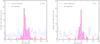 |
Fig. 1 Radial velocity distribution of γ Vel (left panel) and Cha I (right panel) stars. Thick (red) and thin (blue) lines represent the histograms of “lithium members” and targeted nonmembers, respectively. Lithium members fulfilling also the RV criterion are represented by the red hatched area. In γ Vel there is a double peak in the RV distribution of members and a total absence of such peaks for nonmembers. |
The spectra observed in the γ Vel and Cha I fields, which are publicly available3, have been analyzed by the GES working groups WG8 and WG12. WG8 derives radial velocity (RV) and projected rotational velocity (vsini) both for GIRAFFE (Jeffries et al. 2014) and UVES spectra (Sacco et al. 2014). WG12 is the working group responsible for analyzing PMS clusters, and it delivers spectral type (SpT), effective temperature (Teff), surface gravity (log g), vsini (derived with a different approach than WG8), iron abundance ([Fe/H]), microturbulence (ξ), veiling (r), lithium EW at λ6707.8 Å (EWLi), lithium abundance (log nLi), Hα/Hβ EWs (EWHα/EWHβ) and fluxes (FHα/FHβ), Hα full width at 10% of peak height (10%WHα), mass accretion rate (Ṁacc), and other elemental abundances ([X/H]).
2.1. Member selection
For the γ Vel cluster, WG8 produced reliable values of RV and vsini for most of the 1242 targets observed with GIRAFFE. The analysis performed by WG12, which is restricted to spectra with a signal-to-noise ratio S/N ≥ 20, provided values of the main stellar parameters (SpT, Teff, log g) for 1078 stars. Among the 80 stars observed with UVES, the stellar parameters were determined for 68 stars, the remaining being spectroscopic binaries (six stars) or early-type and rapidly rotating stars.
For the 674 stars observed with GIRAFFE in the Cha I field, WG12 released values of the main stellar parameters for 556 of them, while 42 out of the 48 UVES sources have atmospheric parameter entries in the GESviDR1Final catalog. As for γ Vel, the fundamental parameters were not derived for the double-lined spectroscopic binaries (SB2s), the early-type and rapidly rotating stars, and all the sources that have a spectrum with S/N< 20.
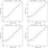 |
Fig. 2 Results of the Monte Carlo simulations on vsini made with GIRAFFE spectra of two slowly-rotating stars for S/N = 100 (upper panels) and S/N = 20 (lower panels). The average vsini measured with our procedure (dots) are plotted against the “theoretical” vsini to which the spectra have been broadened. The one-to-one relation is plotted with a dotted line. |
In the following, we use the membership criteria adopted by Jeffries et al. (2014) for γ Vel and Spina et al. (2014b) for Cha I. The selection performed by these authors was based on the strength of the lithium line at λ6707.8 Å (a reliable indicator of membership in young clusters), the surface gravity (to identify and discard lithium-rich giant contaminants in the field), and the position in the color-magnitude diagram (CMD, to recognize the cluster sequence). We refer to the objects preselected with these criteria as “lithium members”. The final members are those that fulfill an additional criterion based on their radial velocity: 8 ≤ RV ≤ 26 km s-1 for γ Vel and 10 ≤ RV ≤ 21 km s-1 for Cha I (see Fig. 1). The reader is referred to these papers for a broad description of the membership analysis and the selection criteria. The only difference with respect to these works is that we have slightly fewer targets, because we have restricted the analysis for deriving stellar parameters and chromospheric emission to the spectra with a S/N higher than 20. The RV distribution of the lithium members and targeted nonmembers of γ Vel and Cha I clusters, according to the above criteria is displayed in Fig. 1. The finally selected members are represented by the hatched areas in the histograms of Fig. 1.
The parameters for the members of γ Vel and Cha I clusters are reported in Tables 2 and 3, respectively.
In the end, our study is based on 132 members of γ Vel cluster observed only with GIRAFFE (154 lithium members) and on eight lithium members observed with UVES; six of them are also RV members and two are also observed with GIRAFFE. For Cha I, our analysis is based on 59 GIRAFFE and 15 UVES members. We notice that the SB2s, which are identified by means of the cross-correlation functions, are not included in our study. However, the SB2s in our sample are rather few (28 in γ Vel and 6 in Cha I) in comparison to the total number of targets (both members and nonmembers) and most of them cannot be considered as candidate members on the basis of lithium. Thus, we do not expect that their exclusion would have appreciably biased our sample. The same occurs for the rejection of the low S/N spectra. Compared to the 208 lithium members of γ Vel reported by Jeffries et al. (2014), we have 54 fewer stars, i.e., our sample is roughly three quarters the size of theirs. We are missing mostly some of the coolest stars, but this cut should have not biased the sample with respect to rotation velocity, Hα flux, and accretion.
3. Analysis
3.1. Projected rotation velocity and veiling
In the GES analysis of PMS clusters, SpT, vsini, and veiling are produced by one analysis node of WG12 that makes use of ROTFIT, an IDL4 code developed for deriving SpT, Teff, log g, [Fe/H], r, and vsini for the targets. This code compares the target spectrum with a grid of templates composed of high-resolution (R ≃ 42 000) spectra of 294 slowly rotating, low-activity stars retrieved from the ELODIE Archive (Moultaka et al. 2004). The templates were brought to the GIRAFFE resolution, aligned in wavelength with the target spectrum by means of the cross-correlation, resampled on its spectral points and artificially broadened by convolution with a rotational profile of increasing vsini until the minimum of χ2 is reached (see Frasca et al. 2003, 2006). The list of templates that includes their spectral type and atmospheric parameters is reported in Table 4.
To verify the ability of the procedure to derive the vsini and to check the minimum detectable value with GIRAFFE spectra, we ran Monte Carlo simulations with two slowly-rotating stars, namely 18 Sco (G2 V) and δ Eri (K0 IV). The GIRAFFE spectra of these stars were artificially broadened by convolution with a rotation profile of increasing vsini (in steps of 2 km s-1) and a random noise corresponding to S/N = 20, and S/N = 100 was added. We made 100 simulations per each vsini and S/N by running ROTFIT on every simulated spectrum. After the first nearly flat part where the vsini is unresolved, the linear trend between measured and “theoretical” vsini starts at 6–8 km s-1 (Fig. 2). We thus consider all the vsini values lower than 7 km s-1 as upper limits.
As mentioned above, the vsini for the GIRAFFE spectra is also measured, with a different procedure by WG8 along with the RV determination and the data are stored in the VELCLASS fits extension of the reduced spectra. The results of both procedures are compared for the stars in the γ Vel field in Fig. 3. The overall agreement between the two sets of values is apparent; however, in this study we use the vsini values released by WG12.
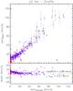 |
Fig. 3 Comparison between the vsini measured by the VELCLASS (WG8) and ROTFIT (WG12) procedures for the stars in the γ Vel field. The ROTFIT’s vsini values lower than 7 km s-1 are denoted by red crosses. |
The code ROTFIT is also able to evaluate the veiling of the spectra. We have left r free to vary in the code only when a veiling can be expected, i.e. for objects with a likely accretion, because this greatly increases the computing time. In the WG12, the “accretor candidates” are selected as those stars with 10%WHα ≥ 270 km s-1 (White & Basri 2003). However, for these two young clusters, we preferred to use less restrictive criteria to check whether a significant veiling can also be found by the code for objects just under the above cutoff. Thus, we ran the code with the veiling option enabled for all objects with 10%WHα ≥ 200 km s-1. We found a handful of objects with 200 < 10%WHα< 270 km s-1 and a nonzero veiling, all of which with r< 0.25, so probably not significant. The uncertainty of veiling determinations is in the range 20–50% whenever r> 0.25 (see Tables 2 and 3).
When searching for the best templates to reproduce the veiled stars, we considered the following equation: 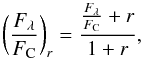 (1)where Fλ and FC represent the line and continuum fluxes, respectively. Moreover, r was left free to vary to find the minimum χ2, assuming that it is constant over a limited wavelength range (which is 100 Å for the 18 UVES spectral segments independently analyzed and about 300 Å for the GIRAFFE spectra). In Fig. 4 we show an example of an accreting star in Cha I with r = 0.4, as found by ROTFIT.
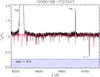 |
Fig. 4 UVES spectrum of an accreting star in Cha I (thick black line) with overplotted the rotationally-broadened and veiled best template (thin red line). A wavelength independent veiling of 0.4 (hatched area) was found by ROTFIT. |
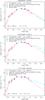 |
Fig. 5 Spectral energy distributions (dots) of two members of the γVel cluster (upper and middle panels) and one member of the young Cha I association (lower panel). In each panel, the best fitting low-resolution NextGen spectrum (Hauschildt et al. 1999) is displayed by a continuous line. The SEDs of the two accretors (middle and lower panels) display MIR excess typical of Class II sources. |
We want to point out that the veiling is better and safer when determined from the UVES spectra than from the GIRAFFE ones because the former have a much wider spectral coverage and include several strong lines suitable for measuring this parameter. This is confirmed by the internal agreement between values of veiling derived from adjacent segments (see also Biazzo et al. 2014). In the case of HR15N GIRAFFE spectra, we can only obtain a rather rough estimate of veiling.
3.2. Spectral energy distribution
To obtain the stellar bolometric luminosities of all analyzed members of γ Vel and Cha I, we constructed the SED of the targets using the optical and near-infrared (NIR) photometric data available in the literature.
For the γ Vel stars, we combined optical BVIC (Jeffries et al. 2009) and 2MASS JHKs (Skrutskie et al. 2006) photometry. Moreover, Spitzer MIR data from Hernández et al. (2008) were also available for about 79% of the sources. For the objects in Cha I, we used BVR photometry from the NOMAD catalog (Zacharias et al. 2004) and Cousins IC magnitudes from the DENIS database that were combined with 2MASS JHKs and Spitzer data (Luhman et al. 2008).
We then adopted the grid of NextGen low-resolution synthetic spectra, with log g in the range 3.5–5.0 and solar metallicity by Hauschildt et al. (1999), to fit the optical-NIR portion (from B to J band) of the SEDs, similar to what was done by Frasca et al. (2009) for stars in the Orion nebula cluster.
For the stars in the γ Vel cluster, we adopted the distance of 360 pc and the extinction AV = 0.131 mag found by Jeffries et al. (2009) and fixed the effective temperatures of the targets to the values found by the spectral analysis of WG12 and delivered in the first internal data release (iDR1). We let the stellar radius (R⋆) vary until a minimum χ2 was reached. The stellar luminosity was then obtained by integrating the best-fit model spectrum. We found a poor SED fitting only for three members of the cluster, J08101877–4714065, J08114456–4657516, and J08110328–4716357. This was likely due to a bad Teff determination. For these stars we instead used the photometric temperatures that are derived as described in Lanzafame et al. (2015). For the members of Cha I, which are scattered in a wide sky region with dense molecular clouds, we made the fit of the SEDs with the extinction parameter free to vary. The SEDs of two members of γ Vel, with and without MIR excess, and one of Cha I are shown, as an example, in Fig. 5.
To our knowledge, no spectroscopic determination of effective temperaure from spectroscopy is available in the literature for the members of γ Vel, while for several objects in Cha I, Luhman (2007) reports SpT, along with the corresponding Teff values, derived from low-resolution spectroscopy. The comparison between our Teff values and Luhman’s shows good agreement in the low temperature domain (Teff< 3800–4000 K), while a systematic difference appears for warmer stars in the sense that Luhman’s values are lower than ours by 200–400 K (up to 800 K in the worst case). We think that the different spectral range and the lower resolution of Luhman’s spectra can be responsible for this discrepancy. Moreover, some scatter could also be introduced by the binarity of a few sources (e.g., Nguyen et al. 2012; Daemgen et al. 2013). The bolometric luminosities, compared to the values reported by Luhman (2007), do not show any relevant offset (≈−13%), but the rms deviation is rather large (≈66%).
3.3. HR diagram
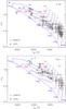 |
Fig. 6 HR diagram of γ Vel (upper panel) and Cha I (lower panel) members for both UVES and GIRAFFE data. The evolutionary tracks of Baraffe et al. (1998) are shown by solid lines with the labels representing their masses. Similarly, the isochrones (from 1 to 30 Myr) by the same authors are shown with dashed lines. The ZAMS position is also represented by a solid line. |
In Fig. 6, we report the position of our targets in the HR diagram, along with the PMS evolutionary tracks and isochrones calculated by Baraffe et al. (1998). The effective temperatures are those from the WG12 analysis delivered in the iDR1, while the stellar luminosities are derived from the SED analysis illustrated in Sect. 3.2. Most of the γ Vel stars are located between the isochrones at 4 and 30 Myr, while the Cha I members lie higher in the diagram, as expected according to their younger age.
We used the HR diagram and the evolutionary tracks for estimating the masses of the targets by minimizing the quantity: 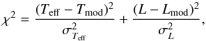 (2)where Teff and σTeff are the stellar effective temperature and its error, respectively, and Tmod is the temperature of the nearest evolutionary track. Analogously, L and σL are the stellar bolometric luminosity and its error, respectively, while Lmod is the luminosity of the nearest track.
The masses, which are also reported in Tables 2 and 3, are used in Sect. 3.5 to evaluate the mass accretion rate.
3.4. Equivalent width and flux of the Hα and Hβ lines
The most useful indicator of chromospheric activity in the HR15N GIRAFFE setup is the Hα line, while the UVES spectra include, among other diagnostics, the Hβ line. Unlike the chromospheric and transition region lines at ultraviolet wavelengths, the contribution of the photospheric flux in these optical lines is very important and must be removed to isolate the pure chromospheric emission that often is only filling in the line cores. Thus, for the WG12 analysis, we have calculated EWs and fluxes by using the spectral subtraction method (see, e.g., Frasca & Catalano 1994; Montes et al. 1995, and references therein) to remove the photospheric flux and emphasize the chromospheric emission in the line core (see Fig. 7). Thanks to this procedure, the net EW of the Hα and Hβ lines (EWHα, EWHβ) were derived (see Tables 2, 3, and 5). In the example shown in Fig. 7, the Hα line is totally filled in by emission and its core just reaches the continuum level, while the Hβ emission that fills in the line core is only detected after subtracting the low-activity template. In both the Hα and Hβ regions, the photospheric absorption lines are mostly removed by the subtraction.
Whenever a veiling r> 0 was found, it has been introduced in the low-activity template before the subtraction, following Eq. (1), so as to reproduce the photospheric lines of the target. However, the EWs reported in Tables 2 and 3 and stored in the GESviDR1Final catalog are not corrected for veiling. To obtain the corrected values, they must be multiplied by (1 + r).
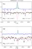 |
Fig. 7 Example of the spectral subtraction method with UVES spectra in the Hα (upper panel) and Hβ (lower panel) regions for an active star in γ Vel. The target spectrum is represented by a solid black line, while the best-fitting reference spectrum of a low-activity star artificially broadened at the vsini of the target is overplotted with a thin red line. In both panels, the difference spectrum (blue line) is displayed as shifted upward by 1.3 for clarity. The residual Hα and Hβ profiles integrated over wavelength (hatched green areas) provide the net equivalent widths (EWHα and EWHβ). The narrow absorption features visible in the upper panel are telluric water-vapor lines. |
The EWHα is plotted as a function of Teff for members of γ Vel and Cha I in Fig. 8. The largest EWHα are observed for cooler stars owing to contrast effects (i.e., the Hα emission stands out against a low continuum level). This behavior is commonly observed in young clusters and associations (see, e.g. Stauffer et al. 1997; Kraus et al. 2014).
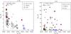 |
Fig. 8 Net Hα equivalent width versus Teff of the γ Vel (left panel) and Cha I (right panel) members observed with GIRAFFE and UVES. The symbol size scales with the vsini. Filled symbols denote the accretor candidates (10%WHα> 270 km s-1), while the targets with a significant amount of veiling (r ≥ 0.25) are enclosed in open squares. The two arrows represent the targets with EWHα out of the range. |
A better diagnostic of chromospheric activity is the line surface flux (indicator of radiative losses), which can be derived from the net line EW as  where F6563 and F4861 are the continuum surface fluxes at the Hα and Hβ wavelengths, respectively, and they are evaluated from the NextGen synthetic low-resolution spectra (Hauschildt et al. 1999) at the stellar temperature and surface gravity provided by the GES consortium.
As a further activity index, we have also calculated the ratio of the chromospheric emission in the Hα line to the total bolometric emission:  (5)The behavior of the activity indicators as a function of stellar parameters is described in Sects. 4.2 and 4.3.
3.5. Mass accretion rate diagnostics
As mass accretion rate (Ṁacc) for the members of both clusters, we considered the values reported by the GES consortium in the iDR1 (see Lanzafame et al. 2015), which are based on the measurements of the 10%WHα performed on the observed Hα profiles, without subtracting the low-activity template. The values of Ṁacc were computed using the Natta et al. (2004) relationship: (6)with 10%WHα in km s-1 and Ṁacc in M⊙ yr-1. Typical errors in log Ṁacc from this relation are about 0.4 − 0.5 dex. Natta et al. (2004) provide this relation for objects with 10%WHα> 200 km s-1, corresponding to log Ṁacc ~ − 11. For this reason, the GES data contains Ṁacc for stars with 10%WHα> 200 km s-1, but only the objects that meet the most restricted criterion, 10%WHα> 270 km s-1 (White & Basri 2003), are considered as accretor candidates.
An independent way of deriving the mass accretion rate is based on the total energy flux in emission lines. We used the empirical relations between accretion luminosity (Lacc) and the luminosity in the Hα line (LHα), which have been recently derived by Alcalá et al. (2014) from X-Shooter at VLT data to estimate Lacc. The line luminosity was calculated as  , where the stellar radius (R⋆) was derived from the analysis of the SEDs (Sect. 3.2), while the surface flux (FHα) was obtained using the net EW of the Hα line, as described in Sect. 3.4. Unlike several previous works, we have decided to use the net Hα EW, where we have removed the contribution of the photospheric line absorption, to have a single diagnostic for both the chromospheric emission and accretion, which are simultaneously investigated. This choice allows us to properly treat the stars with a faint emission or only a filled-in line core. However, for the spectra showing the line as a pure emission feature above the continuum, we also measured the EW of the Hα line without subtracting the low-activity template. We found a negligible flux difference (within 0.1 dex), between EWs from subtracted and unsubtracted spectra, for all the accreting objects, suggesting that the flux calculated with the net EWs can be safely used in comparison with previous works.
The mass accretion rate (Ṁacc) was then derived from Lacc using the relationship by Hartmann (1998):  (7)where the stellar mass M⋆ for each star was estimated from the theoretical evolutionary tracks, as described in Sect. 3.3, and the inner-disk radius Rin was assumed to be Rin = 5R⋆ (Hartmann 1998). Contributions to the error budget on Ṁacc include uncertainties on stellar mass, stellar radius, inner-disk radius, and Lacc. Assuming mean errors of ~0.15 M⊙ in M⋆ and ~0.1 R⊙ in R⋆, 5–10% as relative error in EWHα, 10% in the continuum surface flux at the Hα line used for deriving FHα, and the uncertainties in the relationships by Alcalá et al. (2014), we estimate a typical error in log Ṁacc of ~0.5 dex.
The use of the Hα EW allows us to define as “confirmed accretors” those objects that fulfill the requirements proposed by White & Basri (2003, see their Fig. 7) and based on both Hα EW and SpT. Adopting these criteria, we identified 26 and 3 accretors in Cha I and γ Vel, respectively. Similar results are found adopting the selection criteria proposed by Barrado y Navascués & Martín (2003, see their Fig. 5). We point out that 24 out of 26 accretors in Cha I were classified as flat or Class II IR sources by Manoj et al. (2001) and Luhman et al. (2008). For the two remaining objects no IR classification is available in the literature. We classified 5 Cha I and 3 γ Vel members, which are close to the border line proposed by White & Basri (2003) or Barrado y Navascués & Martín (2003), as “possible accretors”. All but one of the five possible accretors in Cha I are Class II objects, while the source J11071915–7603048 is a Class III star (Luhman et al. 2008) with 10%WHα ~ 370 km s-1, vsini ~ 10 km s-1, and EWHα = 15.2 Å (see Table 3). Two out of our eight confirmed or possible accretors in γ Vel are reported as Class II objects by Hernández et al. (2008), while all the remaining six sources are classified as Class III.
In Fig. 9, the comparison of the two accretion rate estimates is shown. The difference between the two determinations of Ṁacc for a given object is quite large (~0.8 dex for Cha I and ~0.7 dex for γ Vel, on average). Similar results were also found by Costigan et al. (2012), who studied the variability of mass accretion in a sample of ten stars in Cha I. The same authors suggest that the 10%WHα does not give reliable estimates of average accretion rates, especially when single-epoch observations were performed. The inconsistencies we found between the two Ṁacc determinations may also be due to the effects of Hα extra-absorption by stellar winds on the emission line profile produced by the accretion flow, and to line emission not due to accretion, which can affect the 10% width and the Hα EW in a very different way. For instance, an extra absorption wing that produces a strongly asymmetric or a P-Cygni profile could cause an underestimate of the 10% width that is much larger than for the Hα EW. A Spearman’s rank correlation analysis (Press et al. 1992) applied to the Cha I data provides a coefficient ρ = 0.10 with a significance of its deviation from zero σ = 0.61 which confirms the large data scatter.
For our Cha I data, most of the spread is due to seven stars showing differences in the accretion rates larger than 1 dex. In particular, for the three stars with  dex, namely J11092379–7623207, J11071206–7632232, and J11075809–7742413 (with vsini of some km s-1), the difference is most probably due to the presence of wide wings and/or strong central reversals in their spectra at the epoch of our observations. This overestimates the 10%WHα and, therefore, the mass accretion rate derived from this diagnostic. For the four stars with
 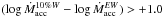 dex, the difference between the two Ṁacc values could be due instead to the Natta et al. (2004) relation in this range of values. In fact, as pointed out by Alcalá et al. (2014), for objects with 10%WHα< 400 km s-1, the Natta et al. (2004) relation tends to underestimate Ṁacc by ~0.6 dex with respect to the determinations coming from primary diagnostics, such as the continuum-excess modeling; however, the differences may be up to about one order of magnitude. Indeed, the stars in our sample with dex have 270 < 10%WHα ≲ 440 km s-1. Herczeg & Hillenbrand (2008), Fang et al. (2009), and Costigan et al. (2012) report similar findings for Taurus, L1641, and Cha I, respectively.
Concerning the data that we acquired for γ Vel, only the possible accretor J08105600–4740069 shows 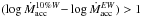 dex. This source displays wide Hα wings, 10%WHα close to 400 km s-1, and a moderate rotation rate (vsini ~ 15 km s-1). It is also a Class II object according to Hernández et al. (2008).
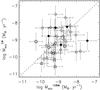 |
Fig. 9 Accretion rates from EWHα versus accretion rates from 10%WHα for Cha I (diamonds) and γ Vel (triangles) stars. Empty and filled symbols refer to GIRAFFE and UVES data, respectively. Squares show the possible accretors. The dashed line is the one-to-one relation. |
4. Results and discussion
4.1. Projected rotation velocity
The availability of a large dataset of cluster members with measured projected rotational velocity allows us to investigate the distribution of stellar rotation rates and their dependence on fundamental stellar parameters.
Figure 10 shows the distribution of vsini for both clusters. The vsini was measured for all 132 GIRAFFE members of the γ Vel cluster according to the three criteria adopted by Jeffries et al. (2014), namely CMD, lithium line, and RV. We also have vsini determinations for the eight late-type members of γ Vel observed with UVES. Two of them have a RV that is not compatible with the cluster, but they fulfill all the other criteria and are considered as members by Spina et al. (2014a). Two of these eight UVES targets have also been observed with GIRAFFE in different observing blocks, but in this study we considered the UVES data for them. The vsini distribution (left panel in Fig. 10) displays a main peak at about 10 km s-1 with a tail toward faster rotators. Despite the blurring of the distribution produced by the inclination angles, compared to a rotation period distribution, its appearance is consistent with a mixture of stars that have spun up and others that have maintained a slow rotation rate likely due to efficient disk locking. We constructed the vsini distributions for the stars that can be unambiguously associated with each of the two kinematical populations identified by Jeffries et al. (2014) and clearly revealed by the double-peaked distribution of the radial velocities (see Fig. 1). Population A, centered at about 16.7 km s-1 with an intrinsic dispersion σA = 0.34 km s-1, is found to be older by about 1–2 Myr than Component B, which is centered at 18.8 km s-1 and shows a wider dispersion (σB = 1.60 km s-1). As already noted by the same authors, the stars in Population B tend to rotate faster, on average, than those of Population A. A two-sided Kolmogorov-Smirnov (KS; Press et al. 1992) test of the cumulative vsini distributions of the two populations reveals a significant difference, with the significance level at PKS = 0.03. This behavior cannot be attributed to the age difference between the two groups, which is too small in comparison with the typical times of rotation evolution and is more likely related to different environmental conditions during their early life. The massive binary system γ2 Vel seems to be slightly younger than the low-mass stars of Population A (Jeffries et al. 2014). Thus, these stars may not have been affected by the strong radiation field and stellar wind from γ2 Vel during the first few Myr of their life, while Population B might have experienced such an effect. As a result, the disks around the members of Population B could have been dispersed earlier than those of Population A, with a shorter disk-locking effect and a faster spin up.
For Cha I, the distribution displays a peak around 10 km s-1, which is narrower than that of γ Vel, and a non-negligible fraction of relatively fast rotators (up to ~40 km s-1). A KS test of the γ Vel and Cha I vsini distributions shows only a marginal difference (PKS = 0.36). This agrees with the results of studies of the evoultion of stellar rotation (e.g., Messina et al. 2010; Spada et al. 2011) that show only a moderate increase in the average rotation rate between the ages of these two clusters.
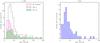 |
Fig. 10 Left panel: distribution of vsini for the members of γ Vel (empty histogram) showing a main peak centered at about 10 km s-1 with a tail towards faster rotators. The two kinematic subsamples A and B identified by Jeffries et al. (2014) display slightly different distributions (hatched and filled histograms), with a higher frequency of faster rotators for Population B. Right panel: distribution of vsini for the members of Cha I, peaked at about 10 km s-1. |
4.2. Hα flux
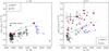 |
Fig. 11 Hα flux versus Teff for the γ Vel (left panel) and the Cha I (right panel) members observed with GIRAFFE and UVES. The symbol size scales with the vsini. The accretor candidates (10%WHα> 270 km s-1) are denoted with filled symbols and typically have a larger flux than the other stars. The candidates that have been rejected on the basis of the EWHα criterion (Sect. 3.5) are marked with crosses. The flux values corrected for veiling by the factor (1 + r) are denoted by arrowheads. In each box, the dashed straight line is drawn to follow the upper envelope of the sources without accretion, while the dotted line is the saturation criterion adopted by Barrado y Navascués & Martín (2003) to separate classical from weak T Tauri. |
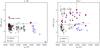 |
Fig. 12
|
In Fig. 11 we show the Hα surface flux as a function of the effective temperature. This figure clearly shows that the nearly exponential behavior displayed by EWHα as a function of Teff (Fig. 8) disappears when the flux is used. In this figure we do not use squares to enclose the stars with a veiling r ≥ 0.25, as we did in Fig. 8, but we display with arrows the flux values obtained by correcting the EWs for the dilution caused by the veiling, i.e. multiplying by the factor (1 + r).
In both panels of Fig. 11 we demarcate the domain of accretors from that of chromospherically active stars. This “dividing line”, which is empirically defined by the upper boundary of the chromospheric fluxes (empty symbols) of stars in both clusters, is expressed by:  (8)For comparison, we also overplotted in Fig. 11 the “saturation limit” adopted by Barrado y Navascués & Martín (2003) for separating classical from weak T Tauri stars; we used the SpT–Teff calibration of Pecaut & Mamajek (2013) for displaying it in a Teff scale. The two boundaries are very close, especially for the coolest stars, where the subtraction of the inactive template has a negligible effect on the FHα owing to both the faint photospheric absorption (compared to usually strong line emissions) and the low continuum flux.
The behavior of  versus Teff for both clusters is displayed in Fig. 12, where a much flatter trend appears. The accretor candidates lie in the upper part of these plots too. The dividing line for this activity index, overplotted with a dashed line, is given by
 (9)We note that the average value of this line is close to the saturation limit,
  , adopted by Barrado y Navascués & Martín (2003) as the boundary between accreting and non-accreting objects, which is also displayed in Fig. 12.
In the case of γ Vel, most stars have FHα close to the maximum values found by Martínez-Arnáiz et al. (2011, see their Fig. 7) for stars with X-ray luminosity in the saturated regime. Moreover, the fluxes do not seem to correlate with the vsini, as indicated by the Spearman’s rank correlation coefficient ρ = 0.057 and by the two-sided significance of its deviation from zero σ = 0.519, even rejecting the few accretors. A higher coefficient (ρ = 0.452) with a σ = 7.6 × 10⁻⁸ is found instead for  versus vsini. This suggests that most stars have already reached the saturation of magnetic activity, while the remaining objects are likely to be contributing to this residual correlation, which is best detected in the diagnostic. Similar results are found for Cha I when the accreting objects are disregarded.
Eight out of the 140 UVES+GIRAFFE members of the γ Vel cluster are accretor candidates (10%WHα> 270 km s-1), but we only confirmed three accretors. The percentage of accretors is then 2 % or, at most, 4 % if we also consider the possible accretors. All these objects fall above or close to the dividing line, while two candidates, namely J08103074–4726219 and J08104649–4742216, lie well below this boundary (see Figs. 11 and 12, left panels). The first one has 10%WHα ~ 280 km s-1 and was finally classified as a nonaccretor. The second one shows a large 10%WHα uncertainty (~30%) due to the bad quality of the spectrum, so it cannot be considered as an accretor according to the criteria adopted in Sect. 3.5. Both are reported as Class III sources by Hernández et al. (2008) based on their SED.
All the members of Cha I with 10%WHα> 270 km s-1 fall above or very close to the dividing line with only two exceptions. One of these two stars is J11085242–7519027 (Teff ~ 3400 K, 10%WHα ~ 272 km s-1), which we finally do not classify as an accretor, while the other, namely J11122441–7637064 (Teff ~ 5100 K and 10%WHα ~ 380 km s-1), is defined as an accretor. Moreover, J11122441–7637064 was previously classified as a classical T Tauri on the basis of Spitzer photometry (e.g., Wahhaj et al. 2010), and Nguyen et al. (2012) report a value of 10%WHα (381 km s-1) that is very close to our measurement. Luhman (2007) finds a lower effective temperature for it (Teff ~ 4660 K) from low-dispersion spectra. If we adopt this temperature, we obtain a flux log FHα ≃ 7.0 (in cgs units) that leads the star slightly closer to the dividing line. However, this star is a visual binary with a companion at about 2″ (Daemgen et al. 2013), whose light could have contaminated the GIRAFFE spectrum.
As mentioned in Sect. 3.1, the veiling was taken as a free parameter only for the stars with strong and broad Hα emission, which was considered as the main requirement for the preselection of accretor candidates within the GES. We found no star in γ Vel with r> 0.25. Among the eight stars with a veiling detection, one is an accretor, and two more are possible accretors according to our definition in Sect. 3.5.
 |
Fig. 13 Hα flux versus veiling for the Cha I members observed with GIRAFFE and UVES. The accretor candidates (10%WHα> 270 km s-1) are denoted by filled symbols, as in Fig. 11. All the stars with a significant veiling (r ≥ 0.5) turn out to be confirmed or possible accretors. The full line is a linear best fit to the data with r ≥ 0.25. |
In Cha I the picture is very different. Among the 74 UVES+GIRAFFE members, 31 sources (about 42 %) display 10%WHα> 270 km s-1 and all are confirmed (26 sources, i.e. 35 %) or possible (5 sources) accretors. Moreover, most of them lie above the line of nonaccreting stars in Fig. 11 by about 0.5–1.0 dex. In addition, as displayed in Fig. 13, all the stars with significant veiling (r ≥ 0.5) are accretors (see also Sect. 4.4). Figure 13 also shows a positive correlation between Hα flux and r, at least for the objects with r ≥ 0.25 for which the Spearman’s rank analysis yields a coefficient ρ = 0.58 with a significance of σ = 0.003. Presently, a more accurate analysis of the stellar properties versus veiling cannot be done because of the uncertainties of the veiling values for GIRAFFE spectra owing to their limited spectral range and the absence of strong photospheric lines in the HR15N setup.
In conclusion, these two clusters are different both in the accretion properties and in the emitted average Hα line flux, with γ Vel showing less accretion signatures than Cha I, as expected by its older age. In particular, the line flux emitted by the confirmed or possible accreting objects in γ Vel is comparable to, or just larger than, the highest chromospheric fluxes emitted by the other γ Vel members, suggesting that most of these stars are near the end of the accretion phase.
4.3. Balmer decrement
The Hα and Hβ fluxes measured in the UVES spectra allowed us to calculate the Balmer decrement (FHα/FHβ) that is a sensitive indicator of the physical conditions, mainly density and temperature, in the emitting regions. The Balmer decrement for the γ Vel and Cha I members is plotted versus Teff in Fig. 14.
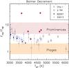 |
Fig. 14 Balmer decrement (FHα/FHβ) versus effective temperature for the γ Vel (triangles) and Cha I (diamonds) stars with residual emission detected both in the Hα and Hβ lines. The accretors are displayed with filled symbols. The decrements measured for late-K and M-type stars by Bochanski et al. (2007, B2007) and Stelzer et al. (2013, S2013) are overplotted with different symbols. The range of values typical of solar plages and of prominences are also shown by the shaded and hatched areas, respectively. |
It is well known that the Balmer decrement for the Sun is quite low (~ 1–2) in the optically thick plasma of plages or preflare active regions, while it is much higher (~ 4.5–12) in the prominences (see, e.g. Tandberg-Hanssen 1967; Landman & Mongillo 1979; Chester 1991).
For the very active giants or subgiants in RS CVn binaries, a Balmer decrement in the range 3–10, i.e. significantly larger than that of solar active regions, has been observed. This has been interpreted as the result of different conditions in the active regions or as the combined effect of plage-like and prominence-like structures (Hall & Ramsey 1992; Chester et al. 1994). For active main-sequence stars, a lower Balmer decrement (in the range 2.2–3.2), but still slightly larger than in solar plages, has been observed (see, e.g. Frasca et al. 2010, 2011). In the case of late-K and M-type stars, a Balmer decrement between solar plages and prominences (2–5), with an increasing trend with the decrease in Teff, has been observed both in field dMe stars (Bochanski et al. 2007) and in PMS Class III stars in regions with age of 1–10 Myr (Stelzer et al. 2013). These data are also displayed in Fig. 14 for comparison.
For the few chromospherically active stars members of γ Vel and for the non-accreting stars in Cha I we also found a Balmer decrement between about two and five, that is, midway between solar plages and prominences. This suggests either that the chromospheric active regions of these young stars have a different structure from the solar plages, mainly as regards their optical thickness, or that the emitted chromospheric flux is the result of contributions from plage-like and prominence-like regions, the latter having a much higher Balmer decrement. Moreover, these data do not show any clear dependence of the Balmer decrement on Teff for the G–K-type stars in 1–10 Myr age range, unlike what is seen for M-type stars (Stelzer et al. 2013).
The star J11064510–7727023 (=UX Cha) was disregarded in this analysis because of unreliable EWHβ value owing to the extremely low S/N of the spectrum in the Hβ region. The six accreting stars in Cha I observed with UVES display instead higher Balmer decrements, from about 3 to 30, as expected from an optically thin accreting matter.
4.4. Mass accretion rate
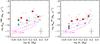 |
Fig. 15 Mass accretion rate from 10%WHα (left panel) and EWHα (right panel) versus stellar mass. Diamonds and triangles represent Cha I and γ Vel stars, where filled and empty symbols refer to UVES and GIRAFFE data, respectively. Squares mark the position of the possible accretors. Big red diamonds represent the median values of Ṁacc for stellar masses of Cha I members binned at 0.2 M⊙, where both confirmed and possible accretors were considered. The dashed line represents the |

In Fig. 15, the mass accretion rates measured by means of the 10%WHα and EWHα diagnostics are plotted as a function of the stellar mass derived from the HR diagram (see Sect. 3.3). From this figure, it is evident how all confirmed and possible accretors in both clusters fall above the boundaries between chromospheric emission and accretion as defined by Manara et al. (2013) for the ages of Cha I and γ Vel (~3 Myr and ~10 Myr, respectively). This means that the selection of accreting objects within the GES is reliable.
Moreover, from the same figure, the large spread in accretion rates is also evident for any given mass similar to what has already been found by previous studies. Short-term (e.g., Biazzo et al. 2012) and long-term variability (up to ~0.5 dex according to Costigan et al. 2014) may contribute to, but not explain, the wide vertical spread of the Ṁacc − M⋆ relationship. Different methodologies for deriving Ṁacc (see e.g., Alcalá et al. 2014) may also contribute to the scatter, but the wide spread (up to 3 dex) observed in the Ṁacc − M⋆ relation is still unexplained. What seems to be reached is the general agreement in finding a dependence of Ṁacc on stellar mass with a power of ~2 (e.g., Muzerolle et al. 2005; Herczeg & Hillenbrand 2008; Alcalá et al. 2014). From Fig. 15, despite the wide spread in Ṁacc at each stellar mass, an increasing trend of Ṁacc with M⋆ seems to be present, and this emerges more clearly when Ṁacc is derived from EWHα. The power-law relation  , which is also depicted in Fig. 15, is consistent with our data, although the scatter does not allow us to say more. A Spearman’s rank correlation analysis yields a coefficient ρ = 0.44 for Cha I with a significance σ = 0.01 for Ṁacc derived from EWHα, indicating a significant positive correlation, while Ṁacc is less correlated with the stellar mass (ρ = 0.26, σ = 0.16) when it is obtained from 10%WHα.
Summarizing, the mass accretion rate for the few accretors in the γ Vel sample ranges from ~10-11 to 10-9 M⊙ yr-1, while for the Cha I members it is in the range 10-10−5 × 10⁻⁸ M⊙ yr-1, with a mean value of ~2 × 10⁻⁹ M⊙ yr-1 at ~1 M⊙. Considering the different ages of γ Vel and Cha I, these values are consistent with the temporal decay of mass accretion rates due to the mechanisms driving the evolution and dispersal of circumstellar disks (see, e.g., Hartmann et al. 1998). Moreover, as mentioned in Sect. 4.2, we find a fraction of accretors of ~35–42% in Cha I and ~2–4% in γ Vel, which are in very good agreement with the results of Fedele et al. (2010) based on low-resolution spectra and consistent with the disk fractions for stellar clusters with ages similar to that of γ Vel and Cha I (Ribas et al. 2014).
A comparison between our mass accretion rates with those derived in the literature is presented in Appendix A.
5. Summary and conclusions
In this paper we used the dataset provided by the GES consortium to study the chromospheric activity and accretion properties of the γ Vel and Cha I regions. Our findings can be summarized as follows:
-
GIRAFFE spectra acquired within the GES survey with aS/N> 20 for stars in the young associations γ Vel and Cha I form statistically significant samples for the analysis of vsini.
-
The vsini distribution for the members of γ Vel appears asymmetric with a main peak at about 10 km s-1 and a broad tail extending toward fast rotators. This suggests the presence of both stars that are at the end of the disk-locking phase and are still rotating rather slowly and others that have started to spin-up while contracting and approaching the ZAMS. Some indication of a distinction between the A and B kinematical subsamples discovered by Jeffries et al. (2014) emerges from the vsini data.
-
We found no clear dependence of the chromospheric Hα flux on vsini. Only a hint of correlation with the vsini emerges instead for
, i.e. the line flux normalized to the bolometric one. This very weak dependence on vsini may be due to activity saturation for most of the non-accreting stars, as witnessed by the high chromospheric fluxes that are comparable to those typical of stars in the saturated regime. -
A low fraction (~2–4%) of γ Vel members display mass accretion, while a much higher percentage (~35–42%) were found for Cha I. This is an expected result based on the quick dissipation of the disks after their typical lifetime of 5–7 Myr, and it suggests that γ Vel is right at the end of the accretion phase.
-
Accreting and active stars occupy two different regions in a Teff–FHα diagram and we propose a simple criterion for distinguishing them, which is, however, very consistent with previous findings (e.g., Barrado y Navascués & Martín 2003). The few stars around the dividing line in our plots are possibly near the end of their accretion phase or have very high chromospheric fluxes.
-
The Balmer decrement (FHα/FHβ) was calculated for the stars observed with UVES, where the setup included both Hα and Hβ. In the case of the active stars in γ Vel and the nonaccreting members of Cha I, we found values in the range 2–5, which are slightly higher than those observed in solar plages, as already found in other very active stars. This indicates either that the chromospheric active regions are not as optically thick as in the Sun or that the hemisphere-averaged chromospheric emission is the result of a “mixture” of plage-like and prominence-like regions, the latter having a much higher Balmer decrement. All the few accreting stars in Cha I observed with UVES display a Balmer decrement of ~5–30, indicating an optically thin emission from the accreting matter.
-
The accreting stars in Cha I display a wide range of r values, but all the stars for which we found a veiling greater than 0.25 are accretors.
-
On the one hand, the luminosity in the Hα line proved to be a more reliable diagnostic than the Hα 10% width for deriving the mass accretion rate, as found in previous works. On the other hand, the Hα 10% width represents a fast and efficient criterion for selecting accretor candidates for ad hoc analysis, for example by searching for the value of veiling that, in combination with that of other free parameters, matches the observations best.
In conclusion, the results presented in this work, which are based on the first two young clusters observed by the GES, show the huge potential of the survey for studying the fundamental properties of PMS stars, such as their rotation, magnetic activity, and mass accretion properties as a function of basic stellar parameters like mass and age. This type of analysis can be extended to the other young clusters that are being observed within the GES. This will provide an unprecedented picture of these phenomena in low-mass stars during the first stages of their evolution.
Online material
Hβ equivalent widths and fluxes for the members of γ Vel and Cha I observed with UVES.
Mass accretion rates derived in the literature with different methods.
Appendix A: Cha I: comparing  with the literature
In Fig. A.1, we compare the mass accretion rates from the literature with those computed in this work from the Hα EW (see also Table 6).
Hartmann et al. (1998) derived mass accretion rates from intermediate-resolution spectrophotometry of the hot continuum emission. Ten accretors are shared with us. Our values and those obtained by these authors agree within the errors with the only exception of J11072825–7652118, for which our Ṁacc is lower than the Hartmann et al. (1998) value by ~1.7 dex, but it is close to the values reported by other authors (see Daemgen et al. 2013). Three accretors of our sample have also been observed by Kim et al. (2009), who measured Ṁacc through U-band photometry. Differences between these values and our determinations are within ~0.3 dex, on average. Recently, Espaillat et al. (2011) have measured Ṁacc with a similar method to the latter authors; for the four accretors in common with, us a mean difference of ~0.5 dex is found. Seven accreting objects are shared with Antoniucci et al. (2011), who measured Ṁacc through the Brγ line. Four stars show similar mass accretion rates, while the values for the three targets with the lowest Ṁacc are higher than ours. Similar differences have also been found by Biazzo et al. (2012) for low-mass stars in Chamaeleon II. Robberto et al. (2012) have derived Ṁacc from Hα photometry for five accretors of our sample. The mean difference in Ṁacc between theirs and our value is ~0.7 dex. Costigan et al. (2012) report Ṁacc measurements using three different diagnostics (EWHα, 10%WHα, and EWCa ii − λ8662) for four accretors in common with us. The agreement between their results and ours is good, especially when we consider the Ṁacc derived from their EWHα. The case of J11075809–7742413 is emblematic because they measure the highest difference in Ṁacc derived through the three methods, but the value obtained with EWHα is very close to ours. This suggests that the discrepancies in the Ṁacc values are mostly due to the method used for deriving it rather than to the different instrumentation used or to an intrinsical variability of the source. Finally, Daemgen et al. (2013) have observed three accretors in common with us and have adopted the Brγ line as diagnostics. The agreement with our values is fairly good, with the exception of 10555973–7724399 for which they have derived log Ṁacc = −7.4 M⊙ yr-1 at odds with our value of −9.1 M⊙ yr-1, which is more similar, within the errors, to the values of −8.8 M⊙ yr-1 and −8.4 M⊙ yr-1 obtained by Robberto et al. (2012) and Hartmann et al. (1998), respectively.
In conclusion, we think that the comparison between our Ṁacc, as derived from the Hα luminosity, and the literature values is in general quite good. The differences/inconsistencies can be attributed to intrinsic short-term and long-term variability (as outlined in Sect. 4.4) and the different photometric/spectroscopic methodologies used by each author to derive accretion luminosity and the mass accretion rate, as well as to the different evolutionary models adopted to estimate the stellar parameters (as also recently pointed out by Alcalá et al. 2014).
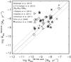 |
Fig. A.1 Comparison between our Ṁacc values calculated using the EWHα and those obtained by several authors. Dashed and dotted lines represent the one-to-one relation and the position of the typical mean error in Ṁacc of ± 0.5 dex. The legend in the upper left corner explains the meaning of the symbols. |
IDL (Interactive Data Language) is a registered trademark of Exelis Visual Information Solutions.
Acknowledgments
The authors are grateful to the referee for carefully reading the paper and for the useful remarks. This work was partly supported by the European Union FP7 program through ERC grant number 320360 and by the Leverhulme Trust through grant RPG-2012-541. We acknowledge the support from INAF and Ministero dell’Istruzione, dell’ Università e della Ricerca (MIUR) in the form of the grant “Premiale VLT 2012”. The results presented here benefit from discussions held during the Gaia-ESO workshops and conferences supported by the ESF (European Science Foundation) through the GREAT Research Network Program. S.G.S. acknowledge the support from the Fundação para a Ciência e Tecnologia, FCT (Portugal) in the form of the fellowship SFRH/BPD/47611/2008. This research also made use of the SIMBAD database, operated at the CDS (Strasbourg, France) and of the Deep Near Infrared Survey of the Southern Sky (DENIS) database.
References
- Alcalá, J. M., Natta, A., Manara, C., et al. 2014, A&A, 561, A2 [NASA ADS] [CrossRef] [EDP Sciences] [Google Scholar]
- Antoniucci, S., García-López, R., Nisini, B., et al. 2011, A&A, 534, A32 [NASA ADS] [CrossRef] [EDP Sciences] [Google Scholar]
- Baraffe, I., Chabrier, G., Allard, F., & Hauschildt, P. H. 1998, A&A, 337, 403 [NASA ADS] [Google Scholar]
- Barrado y Navascués, D., Martín, E. L., 2003, AJ, 126. 2997 [NASA ADS] [CrossRef] [Google Scholar]
- Bayo, A., Barrado, D., Huélamo, N., et al. 2012, A&A, 547, A80 [NASA ADS] [CrossRef] [EDP Sciences] [Google Scholar]
- Biazzo, K., Alcalá, J. M., Covino, E., et al. 2012, A&A, 547, A104 [NASA ADS] [CrossRef] [EDP Sciences] [Google Scholar]
- Biazzo, K., Alcalá, J. M., Frasca, A., et al. 2014, A&A, 572, A84 [NASA ADS] [CrossRef] [EDP Sciences] [Google Scholar]
- Bochanski, J. J., West, A. A., Hawley, S. L., & Covey, K. R. 2007, AJ, 133, 531 [NASA ADS] [CrossRef] [Google Scholar]
- Bouvier, J., Forestini, M., & Allain, S. 1997, A&A, 326, 1023 [NASA ADS] [Google Scholar]
- Calvet, N., Briceno, C., Hernández, J., et al. 2005, AJ, 129, 935 [CrossRef] [Google Scholar]
- Chester, M. M. 1991, Ph.D. Thesis, Pennsylvania State Univ. [Google Scholar]
- Chester, M. M., Hall, J. C., & Buzasi, D. 1994, in Eigth Cambridge Workshop on Cool Stars Slettar Systems and the Sun, ed. J.-P. Caillault, ASP Conf. Ser., 64, 1994 [Google Scholar]
- Costigan, G., Scholz, A., Stelzer, B., et al. 2012, MNRAS, 427, 1344 [NASA ADS] [CrossRef] [Google Scholar]
- Costigan, G., Vink, J. K., Scholz, A., Ray, T., & Testi, L. 2014, MNRAS, 440, 3444 [NASA ADS] [CrossRef] [Google Scholar]
- Daemgen, S., Petr-Gotzens, M. G., Correia, S., et al. 2013, A&A, 554, A43 [NASA ADS] [CrossRef] [EDP Sciences] [Google Scholar]
- Espaillat, C., Furlan, E., D’Alessio, P., et al. 2011, ApJ, 728, 49 [NASA ADS] [CrossRef] [Google Scholar]
- Fang, M., van Boekel, R., Wang, W., et al. 2009, A&A, 504, 461 [NASA ADS] [CrossRef] [EDP Sciences] [Google Scholar]
- Fedele, D., van den Ancker, M. E., Henning, Th., Jayawardhana, R., & Oliveira, J. M. 2010, A&A, 510, A72 [NASA ADS] [CrossRef] [EDP Sciences] [Google Scholar]
- Frasca, A., & Catalano, S. 1994, A&A, 284, 883 [NASA ADS] [Google Scholar]
- Frasca, A., Alcalà, J. M., Covino, E., et al. 2003, A&A, 405, 149 [NASA ADS] [CrossRef] [EDP Sciences] [Google Scholar]
- Frasca, A., Guillout, P., Marilli, E., et al. 2006, A&A, 454, 301 [NASA ADS] [CrossRef] [EDP Sciences] [Google Scholar]
- Frasca, A., Covino, E., Spezzi, L., et al. 2009, A&A, 508, 1313 [NASA ADS] [CrossRef] [EDP Sciences] [Google Scholar]
- Frasca, A., Biazzo, K., Kővári, Zs., Marilli, E., & Çakırlı, Ö. 2010, A&A, 518, A48 [NASA ADS] [CrossRef] [EDP Sciences] [Google Scholar]
- Frasca, A., Fröhlich, H.-E., Bonanno, A., et al. 2011, A&A, 532, A81 [NASA ADS] [CrossRef] [EDP Sciences] [Google Scholar]
- Gilmore, G., Randich, S., Asplund, M., et al. 2012, The Messenger, 147, 25 [NASA ADS] [Google Scholar]
- Hall, J. C., & Ramsey, L. W. 1992, AJ, 104, 1942 [NASA ADS] [CrossRef] [Google Scholar]
- Haisch, K. E., Lada, E. A., & Lada, C. J. 2001, ApJ, 553, 153 [Google Scholar]
- Hartmann, L. 1998, in Accretion Processes in Star Formation (Cambridge Univ. Press) [Google Scholar]
- Hartmann, L., Calvet, N., Gullbring, E., & D’Alessio, P. 1998, ApJ, 495, 385 [NASA ADS] [CrossRef] [Google Scholar]
- Hauschildt, P. H., Allard, F., & Baron, E. 1999, ApJ, 512, 377 [NASA ADS] [CrossRef] [Google Scholar]
- Herbst, W., Bailer-Jones, C. A. L., Mundt, R., Meisenheimer, K., & Wackermann, R. 2002, A&A, 396, 513 [NASA ADS] [CrossRef] [EDP Sciences] [Google Scholar]
- Herczeg, G. J., & Hillenbrand, L. A. 2008, ApJ, 681, 594 [NASA ADS] [CrossRef] [Google Scholar]
- Hernández, J., Hartmann, L., Calvet, N., et al. 2008, ApJ, 686, 1195 [NASA ADS] [CrossRef] [Google Scholar]
- Ingleby, L., Calvet, N., Herczeg, G., et al. 2013, ApJ, 767, 112 [NASA ADS] [CrossRef] [Google Scholar]
- Jeffries, R. D., Naylor, T., Walter, F. M., Pozzo, M. P., & Devey, C. R. 2009, MNRAS, 393, 538 [NASA ADS] [CrossRef] [Google Scholar]
- Jeffries, R. D., Jackson, R. J., Cottaar, M., et al. 2014, A&A, 563, A94 [NASA ADS] [CrossRef] [EDP Sciences] [Google Scholar]
- Kim, K. H., Watson, D. M., Manoj, P., et al. 2009, ApJ, 700, 1017 [NASA ADS] [CrossRef] [Google Scholar]
- Kraus, A. L., Shkolnik, E. L., Allers, K. L., &,Liu, M. C. 2014, AJ, 147, 146 [NASA ADS] [CrossRef] [Google Scholar]
- Lada, C. J., Muench, A. A., Luhman, K. L., et al. 2006, AJ, 131, 1574 [NASA ADS] [CrossRef] [Google Scholar]
- Landman, D. A., & Mongillo, M. 1979, ApJ, 230, 581 [NASA ADS] [CrossRef] [Google Scholar]
- Lanzafame, A. C., Frasca, A., Damiani, F., et al. 2015, A&A, in press [arXiv:1501.4450] [Google Scholar]
- Luhman, K. L. 2007, ApJ, 173, 104 [Google Scholar]
- Luhman, K. L. 2008, in Handbook of Star Forming Regions Vol. II, ed. B. Reipurth, ASP Mon. Publ., 169 [Google Scholar]
- Luhman, K. L., Allen, L. E., Allen, P. R., et al. 2008, ApJ, 675, 1375 [NASA ADS] [CrossRef] [Google Scholar]
- Mamajek, E. E., & Hillenbrand, L. A. 2008, ApJ, 687, 1264 [NASA ADS] [CrossRef] [Google Scholar]
- Manara, C., Testi, L., Rigliaco, E., et al. 2013, A&A, 551, A107 [NASA ADS] [CrossRef] [EDP Sciences] [Google Scholar]
- Manoj, P., Kim, K. H., Furlan, E., et al. 2001, ApJS, 193, 11 [Google Scholar]
- Martínez-Arnáiz, R., López-Santiago, J., Crespo-Chacón, I., & Montes, D. 2011, MNRAS, 414, 2629 [NASA ADS] [CrossRef] [Google Scholar]
- Meibom, S., Mathieu, R. D., & Stassun, K. G. 2009, ApJ, 695, 679 [NASA ADS] [CrossRef] [Google Scholar]
- Messina, S., Pizzolato, N., Guinan, E. F., & Rodonò, M. 2003, A&A, 410, 671 [NASA ADS] [CrossRef] [EDP Sciences] [Google Scholar]
- Messina, S., Desidera, S., Turatto, M., Lanzafame, A. C., & Guinan, E. F. 2010, A&A, 520, A15 [NASA ADS] [CrossRef] [EDP Sciences] [Google Scholar]
- Montes, D., de Castro, E., Fernandez-Figueroa, M. J., & Cornide, M. 1995, A&AS, 114, 287 [NASA ADS] [Google Scholar]
- Moultaka, J., Ilovaisky, S. A., Prugniel, P., & Soubiran, C. 2004, PASP, 116, 693 [NASA ADS] [CrossRef] [Google Scholar]
- Muzerolle, J., Luhman, K. L., Briceño, C., Hartmann, L., & Calvet, N. 2005, ApJ, 625, 906 [NASA ADS] [CrossRef] [Google Scholar]
- Natta, A., Testi, L., Muzerolle, J., et al. 2004, A&A, 424, 603 [NASA ADS] [CrossRef] [EDP Sciences] [Google Scholar]
- Nguyen, D. C., Brandeker, A., van Kerkwijk, M. H., & Jayawardhana, R., 2012, ApJ, 745, 119 [Google Scholar]
- Pace, G. 2013, A&A, 551, L8 [NASA ADS] [CrossRef] [EDP Sciences] [Google Scholar]
- Pace, G., & Pasquini, L. 2004, A&A, 426, 1021 [NASA ADS] [CrossRef] [EDP Sciences] [Google Scholar]
- Pecaut, M. J., & Mamajek, E. E. 2013, ApJS, 208, 9 [NASA ADS] [CrossRef] [Google Scholar]
- Pizzolato, N., Maggio, A., Micela, G., Sciortino, S., & Ventura, P. 2003, A&A, 397, 147 [NASA ADS] [CrossRef] [EDP Sciences] [Google Scholar]
- Pozzo, M., Jeffries, R. D., Naylor, T., et al. 2000, MNRAS, 313, L23 [NASA ADS] [CrossRef] [Google Scholar]
- Preibisch, T., & Feigelson, E. D. 2005, ApJS, 160, 390 [NASA ADS] [CrossRef] [Google Scholar]
- Press, W. H., Teukolsky, S. A., Wetterling, W. T., & Flannery, B. P. 1992, Numerical Recipes, The Art of Scientific Computing (Cambridge University Press), second edition [Google Scholar]
- Randich, S., Gilmore, G., & Gaia-ESO Consortium 2013, The Messenger, 154, 47 [NASA ADS] [Google Scholar]
- Rebull, L. M., Wolff, S. C., Strom, S. E., & Makidon, R. B. 2002, AJ, 124, 546 [NASA ADS] [CrossRef] [Google Scholar]
- Ribas, A., Merín, B., Bouy, H., & Maud, L. T. 2014, A&A, 561, A54 [NASA ADS] [CrossRef] [EDP Sciences] [Google Scholar]
- Robberto, M., Spina, L., Da Rio, N., et al. 2012, AJ, 144, 83 [NASA ADS] [CrossRef] [Google Scholar]
- Sacco, G. G., Morbidelli, L., Franciosini, E., et al. 2014, A&A, 565, A113 [NASA ADS] [CrossRef] [EDP Sciences] [Google Scholar]
- Sicilia-Aguilar, A., Hartmann, L., Calvet, N., et al. 2006, ApJ, 638, 897 [NASA ADS] [CrossRef] [Google Scholar]
- Skumanich, A. 1972, ApJ, 171, 265 [NASA ADS] [Google Scholar]
- Soderblom, D. R., Duncan, D. K., & Johnson, D. R. H. 1991, ApJ, 375, 722 [NASA ADS] [CrossRef] [Google Scholar]
- Spada, F., Lanzafame, A. C., Lanza, A. F., Messina, S., & Collier Cameron, A. 2011, MNRAS, 416, 447 [NASA ADS] [Google Scholar]
- Spina, L., Randich, S., Palla, F., et al. 2014a, A&A, 567, A55 [NASA ADS] [CrossRef] [EDP Sciences] [Google Scholar]
- Spina, L., Randich, S., Palla, F., et al. 2014b, A&A, 568, A2 [NASA ADS] [CrossRef] [EDP Sciences] [Google Scholar]
- Stauffer, J. R., Hartmann, L. W., Prosser, C. F., et al. 1997, ApJ, 479, 776 [NASA ADS] [CrossRef] [Google Scholar]
- Stelzer, B., Frasca, A., Alcalà, J. M., et al. 2013, A&A, 558, A141 [NASA ADS] [CrossRef] [EDP Sciences] [Google Scholar]
- Skrutskie, M. F., Cutri, R. M., Stiening, R., et al. 2006, AJ, 131, 1163 [NASA ADS] [CrossRef] [Google Scholar]
- Tandberg-Hanssen, E. 1967, Solar activity, Waltham, Mass.: Blaisdell [Google Scholar]
- Wahhaj, Z., Cieza, L., Koerner, D. W., et al. 2010, ApJ, 724, 835 [NASA ADS] [CrossRef] [Google Scholar]
- White, R. J., & Basri, G. 2003, ApJ, 582, 1109 [NASA ADS] [CrossRef] [Google Scholar]
- Whittet, D. C. B., Prusti, T., Franco, G. A. P., et al. 1997, A&A, 327, 1194 [NASA ADS] [Google Scholar]
- Zacharias, N., Monet, D. G., Levine, S. E., et al. 2004, Am. Astron. Soc. Meet., 205, #4815, 36, 1418 [Google Scholar]
- de Zeeuw, P. T., Hoogerwerf, R., de Bruijne, J. H. J., Brown, A. G. A., & Blaauw, A. 1999, ApJ, 117, 399 [Google Scholar]
All Tables
Hβ equivalent widths and fluxes for the members of γ Vel and Cha I observed with UVES.
All Figures
|
Fig. 1 Radial velocity distribution of γ Vel (left panel) and Cha I (right panel) stars. Thick (red) and thin (blue) lines represent the histograms of “lithium members” and targeted nonmembers, respectively. Lithium members fulfilling also the RV criterion are represented by the red hatched area. In γ Vel there is a double peak in the RV distribution of members and a total absence of such peaks for nonmembers. |
| In the text | |
|
Fig. 2 Results of the Monte Carlo simulations on vsini made with GIRAFFE spectra of two slowly-rotating stars for S/N = 100 (upper panels) and S/N = 20 (lower panels). The average vsini measured with our procedure (dots) are plotted against the “theoretical” vsini to which the spectra have been broadened. The one-to-one relation is plotted with a dotted line. |
| In the text | |
|
Fig. 3 Comparison between the vsini measured by the VELCLASS (WG8) and ROTFIT (WG12) procedures for the stars in the γ Vel field. The ROTFIT’s vsini values lower than 7 km s-1 are denoted by red crosses. |
| In the text | |
|
Fig. 4 UVES spectrum of an accreting star in Cha I (thick black line) with overplotted the rotationally-broadened and veiled best template (thin red line). A wavelength independent veiling of 0.4 (hatched area) was found by ROTFIT. |
| In the text | |
|
Fig. 5 Spectral energy distributions (dots) of two members of the γVel cluster (upper and middle panels) and one member of the young Cha I association (lower panel). In each panel, the best fitting low-resolution NextGen spectrum (Hauschildt et al. 1999) is displayed by a continuous line. The SEDs of the two accretors (middle and lower panels) display MIR excess typical of Class II sources. |
| In the text | |
|
Fig. 6 HR diagram of γ Vel (upper panel) and Cha I (lower panel) members for both UVES and GIRAFFE data. The evolutionary tracks of Baraffe et al. (1998) are shown by solid lines with the labels representing their masses. Similarly, the isochrones (from 1 to 30 Myr) by the same authors are shown with dashed lines. The ZAMS position is also represented by a solid line. |
| In the text | |
|
Fig. 7 Example of the spectral subtraction method with UVES spectra in the Hα (upper panel) and Hβ (lower panel) regions for an active star in γ Vel. The target spectrum is represented by a solid black line, while the best-fitting reference spectrum of a low-activity star artificially broadened at the vsini of the target is overplotted with a thin red line. In both panels, the difference spectrum (blue line) is displayed as shifted upward by 1.3 for clarity. The residual Hα and Hβ profiles integrated over wavelength (hatched green areas) provide the net equivalent widths (EWHα and EWHβ). The narrow absorption features visible in the upper panel are telluric water-vapor lines. |
| In the text | |
|
Fig. 8 Net Hα equivalent width versus Teff of the γ Vel (left panel) and Cha I (right panel) members observed with GIRAFFE and UVES. The symbol size scales with the vsini. Filled symbols denote the accretor candidates (10%WHα> 270 km s-1), while the targets with a significant amount of veiling (r ≥ 0.25) are enclosed in open squares. The two arrows represent the targets with EWHα out of the range. |
| In the text | |
|
Fig. 9 Accretion rates from EWHα versus accretion rates from 10%WHα for Cha I (diamonds) and γ Vel (triangles) stars. Empty and filled symbols refer to GIRAFFE and UVES data, respectively. Squares show the possible accretors. The dashed line is the one-to-one relation. |
| In the text | |
|
Fig. 10 Left panel: distribution of vsini for the members of γ Vel (empty histogram) showing a main peak centered at about 10 km s-1 with a tail towards faster rotators. The two kinematic subsamples A and B identified by Jeffries et al. (2014) display slightly different distributions (hatched and filled histograms), with a higher frequency of faster rotators for Population B. Right panel: distribution of vsini for the members of Cha I, peaked at about 10 km s-1. |
| In the text | |
|
Fig. 11 Hα flux versus Teff for the γ Vel (left panel) and the Cha I (right panel) members observed with GIRAFFE and UVES. The symbol size scales with the vsini. The accretor candidates (10%WHα> 270 km s-1) are denoted with filled symbols and typically have a larger flux than the other stars. The candidates that have been rejected on the basis of the EWHα criterion (Sect. 3.5) are marked with crosses. The flux values corrected for veiling by the factor (1 + r) are denoted by arrowheads. In each box, the dashed straight line is drawn to follow the upper envelope of the sources without accretion, while the dotted line is the saturation criterion adopted by Barrado y Navascués & Martín (2003) to separate classical from weak T Tauri. |
| In the text | |
|
Fig. 12
|
| In the text | |
|
Fig. 13 Hα flux versus veiling for the Cha I members observed with GIRAFFE and UVES. The accretor candidates (10%WHα> 270 km s-1) are denoted by filled symbols, as in Fig. 11. All the stars with a significant veiling (r ≥ 0.5) turn out to be confirmed or possible accretors. The full line is a linear best fit to the data with r ≥ 0.25. |
| In the text | |
|
Fig. 14 Balmer decrement (FHα/FHβ) versus effective temperature for the γ Vel (triangles) and Cha I (diamonds) stars with residual emission detected both in the Hα and Hβ lines. The accretors are displayed with filled symbols. The decrements measured for late-K and M-type stars by Bochanski et al. (2007, B2007) and Stelzer et al. (2013, S2013) are overplotted with different symbols. The range of values typical of solar plages and of prominences are also shown by the shaded and hatched areas, respectively. |
| In the text | |
|
Fig. 15 Mass accretion rate from 10%WHα (left panel) and EWHα (right panel) versus stellar mass. Diamonds and triangles represent Cha I and γ Vel stars, where filled and empty symbols refer to UVES and GIRAFFE data, respectively. Squares mark the position of the possible accretors. Big red diamonds represent the median values of Ṁacc for stellar masses of Cha I members binned at 0.2 M⊙, where both confirmed and possible accretors were considered. The dashed line represents the |
| In the text | |
|
Fig. A.1 Comparison between our Ṁacc values calculated using the EWHα and those obtained by several authors. Dashed and dotted lines represent the one-to-one relation and the position of the typical mean error in Ṁacc of ± 0.5 dex. The legend in the upper left corner explains the meaning of the symbols. |
| In the text | |
Current usage metrics show cumulative count of Article Views (full-text article views including HTML views, PDF and ePub downloads, according to the available data) and Abstracts Views on Vision4Press platform.
Data correspond to usage on the plateform after 2015. The current usage metrics is available 48-96 hours after online publication and is updated daily on week days.
Initial download of the metrics may take a while.