| Issue |
A&A
Volume 575, March 2015
|
|
|---|---|---|
| Article Number | A30 | |
| Number of page(s) | 25 | |
| Section | Cosmology (including clusters of galaxies) | |
| DOI | https://doi.org/10.1051/0004-6361/201424085 | |
| Published online | 17 February 2015 | |
XMM-Newton and Chandra cross-calibration using HIFLUGCS galaxy clusters
Systematic temperature differences and cosmological impact⋆
1
Argelander-Institut für Astronomie, Universität Bonn,
Auf dem Hügel 71,
53121
Bonn,
Germany
e-mail:
gerrit@uni-bonn.de
2
Tartu Observatory, 61602
Toravere,
Estonia
3
Department of Physics, Dynamicum, PO Box 48, University of
Helsinki, 00014
Helsinki,
Finland
4 Harvard-Smithsonian Center for Astrophysics, 60 Garden
Street, Cambridge, USA
Received: 28 April 2014
Accepted: 3 December 2014
Context. Robust X-ray temperature measurements of the intracluster medium (ICM) of galaxy clusters require an accurate energy-dependent effective area calibration. Since the hot gas X-ray emission of galaxy clusters does not vary on relevant timescales, they are excellent cross-calibration targets. Moreover, cosmological constraints from clusters rely on accurate gravitational mass estimates, which in X-rays strongly depend on cluster gas temperature measurements. Therefore, systematic calibration differences may result in biased, instrument-dependent cosmological constraints. This is of special interest in light of the tension between the Planck results of the primary temperature anisotropies of the cosmic microwave background (CMB) and Sunyaev-Zel’dovich-plus-X-ray cluster-count analyses.
Aims. We quantify in detail the systematics and uncertainties of the cross-calibration of the effective area between five X-ray instruments, EPIC-MOS1/MOS2/PN onboard XMM-Newton and ACIS-I/S onboard Chandra, and the influence on temperature measurements. Furthermore, we assess the impact of the cross-calibration uncertainties on cosmology.
Methods. Using the HIFLUGCS sample, consisting of the 64 X-ray brightest galaxy clusters, we constrain the ICM temperatures through spectral fitting in the same, mostly isothermal regions and compare the different instruments. We use the stacked residual ratio method to evaluate the cross-calibration uncertainties between the instruments as a function of energy. Our work is an extension to a previous one using X-ray clusters by the International Astronomical Consortium for High Energy Calibration (IACHEC) and is carried out in the context of IACHEC.
Results. Performing spectral fitting in the full energy band, (0.7−7) keV, as is typical of the analysis of cluster spectra, we find that best-fit temperatures determined with XMM-Newton/EPIC are significantly lower than Chandra/ACIS temperatures. This confirms the previous IACHEC results obtained with older calibrations with high precision. The difference increases with temperature, and we quantify this dependence with a fitting formula. For instance, at a cluster temperature of 10 keV, EPIC temperatures are on average 23% lower than ACIS temperatures. We also find systematic differences between the three XMM-Newton/EPIC instruments, with the PN detector typically estimating the lowest temperatures. Testing the cross-calibration of the energy-dependence of the effective areas in the soft and hard energy bands, (0.7−2) keV and (2−7) keV, respectively, we confirm the previously indicated relatively good agreement between all instruments in the hard and the systematic differences in the soft band. We provide scaling relations to convert between the different instruments based on the effective area, gas temperature, and hydrostatic mass. We demonstrate that effects like multitemperature structure and different relative sensitivities of the instruments at certain energy bands cannot explain the observed differences. We conclude that using XMM-Newton/EPIC instead of Chandra/ACIS to derive full energy band temperature profiles for cluster mass determination results in an 8% shift toward lower ΩM values and <1% change of σ8 values in a cosmological analysis of a complete sample of galaxy clusters. Such a shift alone is insufficient to significantly alleviate the tension between Planck CMB primary anisotropies and Sunyaev-Zel’dovich-plus-XMM-Newton cosmological constraints.
Key words: X-rays: galaxies: clusters / instrumentation: miscellaneous / galaxies: clusters: intracluster medium / techniques: spectroscopic
Appendices are available in electronic form at http://www.aanda.org
© ESO, 2015
1. Introduction
Galaxy clusters are excellent tools for studying cosmology, in particular the phenomena of dark matter and dark energy, because they are the most massive gravitationally relaxed systems in the Universe. Especially the cluster mass function, which is the number density of clusters with a certain mass, is a sensitive probe of cosmological parameters. By determining the temperature using X-ray emission from the hot intracluster medium (ICM), one traces the most massive visible component of clusters and can derive both the total gravitating mass and the mass of the emitting medium.
Robust cosmological constraints require accurate estimates of the cluster masses without any systematic bias. There are at least two important sources of possible biases in the hydrostatic method: a) the previously reported results of the International Astronomical Consortium for High Energy Calibration (IACHEC)1 on the cross-calibration uncertainties of the effective area between XMM-Newton/EPIC and Chandra/ACIS (Nevalainen et al. 2010, N10), the two major current X-ray missions and b) the hydrostatic bias (e.g., Nagai et al. 2007) whereby a fraction of the total pressure in the ICM has a non-thermal origin, e.g., due to bulk motions. In the latter case, the assumption of the gas pressure balancing the gravity underestimates of the total mass.
Both biases may be affecting the recent Planck results (Planck Collaboration XVI 2014; Planck Collaboration XX 2014), whereby the cosmological constraints driven by the primary temperature anisotropies of the cosmic microwave background (CMB) radiation and Sunyaev-Zel’dovich (SZ) analyses do not agree with each other. For the SZ analysis a relation between the Compton Y parameter and the mass for galaxy clusters derived using XMM-Newton data was used and even allowing for a possible hydrostatic mass bias factor in the range 0.7−1.0, no full agreement between the two probes is achieved. As mentioned before, reasons for the discrepancy can be the breakdown of the hydrostatic assumption, the underestimation of calibration uncertainties in the X-ray, but also in the microwave regime, or an incomplete cosmological model (e.g., the lack of massive neutrinos).
As pointed out in von der Linden et al. (2014), the XMM-Newton-based cluster masses in the Planck sample are significantly lower than the values obtained from a weak lensing analysis. This difference is mass dependent and might be explained by (i) a temperature-dependent calibration uncertainty and/or (ii) a failing hydrostatic assumption. We address the question of whether a Chandra-derived scaling relation could solve this tension, i.e., whether systematic cross-calibration uncertainties between Chandra and XMM-Newton can explain the inconsistent Planck results. The results in Israel et al. (2014a), where Chandra X-ray masses agree with cluster masses of a weak-lensing analysis indicate that the hydrostatic assumption does not cause a major bias with respect to weak-lensing masses. While we clearly isolate here the systematic uncertainty resulting directly and only from X-ray calibration uncertainties, a comparison of mass estimates and/or cosmological constraints from different sources is much more complicated (Rozo et al. 2014).
We show in this work how reliable the current (December 2012) calibrations are by using nearby galaxy clusters as reference objects and comparing the measured XMM-Newton temperatures with the results from Chandra. Galaxy clusters are Megaparsec-scale objects, and their X-ray emission from the hot ICM does not vary on human timescales.
The XMM-Newton/Chandra effective-area cross-calibration uncertainties as reported in N10 yielded that Chandra/ACIS measures ~10–15% higher temperatures in the (0.5−7) keV energy band compared to XMM-Newton/EPIC. Since the N10 sample was relatively small (11 galaxy clusters), it is important to evaluate the XMM-Newton/Chandra effective area cross-calibration uncertainties with a large cluster sample to gain more statistical precision for comparing XMM-Newton and Chandra temperatures. Furthermore, the cosmological implications of cross-calibration uncertainties have not been studied by N10. In more recent works (e.g., Mahdavi et al. 2013; Martino et al. 2014; Donahue et al. 2014) the authors still find significant differences in temperatures between Chandra and XMM-Newton by comparing the data of typically of about of 20 galaxy clusters.
Here we use the HIFLUGCS cluster sample (Reiprich & Böhringer 2002), which provides the 64 galaxy clusters with the highest X-ray flux. High quality Chandra/ACIS and XMM-Newton/EPIC data are available for all of them except one (Hudson et al. 2010; Zhang et al. 2011). This work is an extension of N10 in the sense that it updates the calibration information (as in Dec. 2012) with about five times more objects and that the cosmological impact is quantified. The current data can be used to evaluate both the energy dependence and the normalization of the cross-calibration uncertainties. We are interested in the cross-calibration effect on the cluster mass function, which depends on the temperature and only on the gradient of the gas density. Therefore, the normalization of the effective areas is not relevant for the current work and will be addressed in detail in an upcoming paper.
In this paper we first describe the properties of the galaxy clusters we use in Sect. 2. We give an overview of our data reduction for the two satellites in Sect. 3 and describe the background subtraction in Sect. 4 in more detail. Section 5 deals with the analysis method, and finally we present the results in Sect. 6 and discuss the various effects that might have an influence on the results in Sect. 7. In this section we also describe the cosmological impact on the normalized matter density parameter, Ωm, and the amplitude of the linear matter power spectrum on 8 h-1 Mpc scale, σ8.
Throughout this paper we use a flat ΛCDM cosmology with the following parameters: Ωm = 0.3, ΩΛ = 0.7, H0 = h·100 km s-1 Mpc-1 with h = 0.71.
2. Cluster properties
The whole HIFLUGCS cluster sample consists of 64 clusters with a redshift up to z = 0.215 for RXC J1504. The average redshift of this sample is z = 0.053 with a dispersion of 0.039. All clusters are listed in Table A.1. Chandra/ACIS data are available for all 64 clusters, XMM-Newton/EPIC data for all except A2244, which will be observed in AO13.
In Hudson et al. (2010) a galaxy cluster is defined as a cool-core cluster if the central cooling time is less than 7.7 Gyr. The authors also show that NCC clusters of the HIFLUGCS sample exhibit a temperature drop toward the center of less than 20%, while CC clusters show a decrease in the temperature by a factor of 2 to 5. More details on this phenomenon including the categorization of the HIFLUGCS clusters in CC and NCC clusters can be found in Hudson et al. (2010). To minimize possible biases introduced by multitemperature ICM (Sect. 7.1.1) we exclude the cool core regions of clusters as provided by Hudson et al. (2010) (Table 2).
The greatest limitation for the choice of the extraction region size is imposed by ACIS-S. In order not to lose a fraction of the cluster annulus owing to a relatively limited ACIS-S field of view (FOV), we set the outer extraction radius to 3.5′ around the emission peak, as defined in Hudson et al. (2010).
Finally we always added 15″ on all cool core radii and point-source radii (as determined from Chandra data using a wavelet algorithm) to minimize the scattering of emission into the annulus because of the XMM-Newton PSF. We marked bad columns and chip gaps in the observations of the three EPIC instruments and excluded them from all spectral analyses.
Furthermore, this assures that regions are fully covered by Chandra’s FOV for almost all clusters. All this leads to the following procedure:
-
For cool-core clusters, the cool core region (plus15″) was excluded, and the temperature was measured within an annulus between the cool core and the 3.5′.
-
Non-cool-core clusters are assumed to have no big temperature variations, so the region used here is the full 3.5′-circle. We assume that the azimuthal temperature variations can be neglected for our purpose.
-
For five clusters, the 3.5′ enclose regions outside the ACIS-S chips. Since this could bias our results, we changed the outer border for these clusters (for both XMM-Newton and Chandra) from the usual 3.5′ to a smaller radius that lies completely on the chips. The new outer borders are:
-
2′ for Abell 754
-
2′ for Abell 1367
-
2.1′ for Abell 2256
-
2.4′ for Hydra A
-
2.3′ for NGC 1550.
-
-
For seven clusters2, the cool core is larger than 3.5′. These clusters were excluded from our analysis. To see whether these clusters would bias our result, we analyzed them within the full 3.5′ circle as well (see Fig. 9). The check revealed that these clusters do not show any special behavior in any direction as compared to the other clusters. Apart from the previously mentioned figure and the stacked residual ratio analysis (Sect. 5.2), these seven clusters are always excluded.
Within these regions the source-to-background count-rate ratio in the sample is between 9 and 135 in the (0.7−2.0) keV band.
3. Data processing
3.1. Chandra
Chandra data reduction was performed using the CIAO software (CIAO 4.5, CALDB 4.5.5.1) and the HEASOFT tools (6.12), including the Xspec fitting package (12.7.1d and AtomDB 2.0.2)3. We first created the level-2 event files using the contributed script chandra_repro, for example, to correct for afterglows from cosmic rays. In the next step the chips comprising the selected regions (I-chips were combined for I-observations) were cleaned from solar flares by creating a lightcurve with the suggested values from Markevitch’s Cookbook4 and the lc_clean algorithm. Point sources detected by the wavdetect algorithm were excluded, but each observation was visually inspected for false and insignificant detections, and if necessary, the list of point sources was edited manually. The acis_bkgrnd_lookup script helped us to find the blank-sky background file from the CALDB matching to the observation. Finally background files were reprojected to match the orientation of the cluster observation, before continuing. For VFAINT observations only the events with status bits =0 were used because all background files were taken from VFAINT observations.
Unfortunately, the quiescent particle background varies with time, so we had to compensate for this behavior by rescaling the background count rate with a normalization factor. This factor is the ratio of the count rates in the (9.5−12) keV energy range of the blank sky files and the observations, because the effective area of Chandra is almost zero in this energy interval and almost all events are related to the particle background. This factor is then multiplied by the BACKSCALE value of the background spectral file. To create the spectra and response files, we used the specextract task and created the weighted RMFs and ARFs. The spectra were grouped to have at least 30 counts per bin.
3.2. XMM-Newton
The XMM-Newton data reduction is different in some parts from the Chandra treatment. The software we used was the SAS package version 12.0.1 with CCF calibration files from 14.12.2012. With emchain and epchain, we created the initial event lists excluding flagged events (FLAG==0) and setting PATTERN<=12 for MOS and PATTERN==0 for PN. The decision that only single events be selected for EPIC-PN is because there are still significant gain problems for the double events (see XMM-Newton release note XMM-CCF-REL-309). Blank-sky background files are also available for XMM-Newton and can be downloaded from the website5. One has to make sure to use the correct file for each observation in terms of used filter, pointing and recording mode. Solar flares are a tremendous issue for XMM, so we cleaned the lightcurve in two steps to remove them. To obtain the good time intervals we fitted a Poisson distribution function to a 100 s binned histogram of the high energy lightcurve, i.e. (10−12) keV for MOS and (12−14) keV for PN. Events belonging to a count rate higher than  above the mean count-rate, μ, were rejected.
In a second step, the lightcurve was filtered in the full energy band from (0.3−10) keV by the same method as described. The same thresholds were applied to the background files. We visually inspected all final full-energy band lightcurves and, if necessary, removed strong flares that were not detected by the previously mentioned method. Since Chandra has much better spatial resolution, we used the detected point sources from the Chandra analysis and removed the same regions here. We excluded chip gaps and bad columns of the EPIC instruments from all observations. This exclusion criterion changes the best-fit temperature on the order of 0.5%. The normalization of the background files due to the changing particle background level is done in the same way as for Chandra except that the high energy interval, (9.5−12) keV for Chandra, (10−12) keV for EPIC-MOS and (12−14) keV for EPIC-PN, is different because of Chandra’s lower effective area in the high energy. For the EPIC spectra we used the same spectral grouping parameters as for Chandra of 30 counts per bin.
4. Background treatment
X-ray observations are always contaminated with events not related to the source, which we call background in the following. It usually consists of:
-
the particle background: energetic particles produce charges on the detector while penetrating it, or induce fluorescent emission lines in the surrounding material;
-
the so-called soft protons: these particle events should be removed by the flare reduction process to a significant amount;
-
the cosmic X-ray background (CXB): it can be subdivided into the local hot bubble emission, the thermal emission of the galactic halo, and the contribution of unresolved point sources (most likely AGNs, see, e.g., Hickox & Markevitch 2006);
-
solar wind charge exchange emission (SWCX): highly ionized particles interacting with neutral atoms. For more details, see Wargelin et al. (2004); Snowden et al. (2004).
Generally it is very important to properly account for all background components because they affect the cluster temperature resulting from the spectral fit. The HIFLUGCS clusters are nearby objects, so they cover almost the whole field of view of the two instruments, and the background cannot be estimated from the observation itself. We decided to use the blank-sky observations for both Chandra and XMM-Newton, because our selection criteria ensure that the background is much lower than the source count rate (see Table A.2). These archival observations of regions without astronomical sources are not always the best description for every observation, but when extracting spectra out to only 3.5′ for these very bright objects, the error is negligible, because the background level is at least one order of magnitude lower than the cluster emission. To verify this assumption, we increased the background normalization by 10% up to an energy of 2 keV (see Fig. 1). Beyond that energy the spectrum remains unchanged. This should simulate a different foreground/CXB emission level but leaves the particle background unchanged, which is dominant beyond 2 keV. For ACIS, 91% of the clusters exhibit a difference in the best-fit temperature of less than 2%, while EPIC-PN temperature changes are less than 2% for all clusters. RXC J1504 has a temperature difference for ACIS of almost 3% after changing the background. Still this is not significant, since this cluster is one of the hottest in the sample, and it has a temperature difference between ACIS and EPIC-PN of more than 35% in the full energy band (see Table A.2).
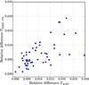 |
Fig. 1 Relative temperature difference resulting from raising the background level by 10% for energies below 2 keV. |
Apart from a systematic under- or overestimation of the background level, an energy dependence of the background spectrum mismatch can be introduced by the photo-electric absorption of the blank sky background: The observations from which the blank sky background is extracted were taken at different sky positions and undergo different absorptions. The mean hydrogen column density along the line of sight, NH, of all these regions will not agree with most of the cluster observation. For all the clusters we checked the effect of changing the background spectra by absorbing it according to the cluster NH minus the exposure-weighted average hydrogen column density of the background file. This method produces a background spectrum as it would have been observed through the cluster line-of-sight absorption. For all clusters the temperature difference is below 3%, and it is below 1% for almost 90% of the clusters. This is also expected since the source to background count rate ratio in the relevant energy band is very high.
In summary, our results are robust against systematic uncertainties in the background estimation.
5. Analysis
5.1. Spectral fitting method
To obtain the emission model and temperature for each region, we fit an apec-model (Smith et al. 2001) and a photoelectric absorption model (phabs) using the cross sections from Balucinska-Church & McCammon (1992). The column density of neutral hydrogen NH and the redshift z are frozen to the values from Zhang et al. (2011), where most of the hydrogen column densities are consistent with the values from the LAB HI survey (Kalberla et al. 2005). For two clusters, Abell 478 and Abell 2163, our spectral fits resulted in a very poor χ2, so we used NH values from spectral fits with the hydrogen column density left free to vary. For Abell 478 we used 3 × 1021 cm-2 and for Abell 2163 2 × 1021 cm-2. Both values are around 100% higher than the LAB values, and they produced a  for the spectral fit. The new values also agree roughly with the NH,tot values, as discussed in Sect. 7.2.
For Abell 478 and Abell 3571, we did not consider the redshifts from Zhang et al. (2011), because all X-ray instruments agree with the new redshift values from the spectral fit (0.0848 instead of 0.0900 for Abell 478 and 0.0374 instead of 0.0397 for Abell 3571).
By default the abundance table presented in Anders & Grevesse (1989, AnGr) was used for the absorption and emission model. Additionally, all values were recomputed using the relative abundance of elements from Asplund et al. (2009, Aspl).
We performed the spectral fits in the full (0.7−7) keV, hard (2−7) keV, and soft (0.7−2) keV energy bands. This is different from the definition in N10, where the low energy threshold of the full and soft bands was at 0.5 keV. We also excluded the events below 0.7 keV to avoid the emission lines around 0.6 keV due to the cosmic X-ray background or SWCX. We also excluded all events above 7 keV because of the prominent EPIC-PN fluorescent lines (Ni at 7.5 keV, Cu at 8 keV, and Zn at 8.6 keV) and the small Chandra effective area. It should be mentioned that the soft band spectral fits for high temperature clusters provides poor constraints on the parameters because the change in the slope of different temperature models is very small, and there are almost no emission lines in this energy band. For the full- and hard-band fits all  are below 1.6, while for the soft band fits the maximum is 2.3 (although for more than 88% the χred are below 1.3). The possibility and influence of a temperature-abundance degeneracy will be discussed in Sect. 7.1.2.
5.2. Stacked residuals ratio
The effective area cross-calibration uncertainties between a pair of instruments as a function of energy can be obtained using the stacked residual ratio method (see Kettula et al. 2013; Longinotti et al. 2008). Using the definition from Kettula et al. (2013) for the stacked residual ratio, 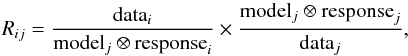 (1)we can test instrument i and use instrument j as reference. We briefly summarize the steps:
-
The results on the relative cross-calibration uncertainties do not depend on the choice of the reference detector.
-
The data of the reference detector are fitted with an absorbed apec-model in the (0.5−7.0) keV energy range. We also experimented by using an absorbed mekal-model to be more consistent with previous works (Kettula et al. 2013; N10) using the stacked residual ratio method, but we did not find any significant differences. This fitting procedure defines our reference model and is not changed any more in the following. We included the (0.5−0.7) keV energy band for the stacked residual ratio test in order to stay close to previous analyses.
-
Each spectral data point of all the instruments (ACIS-S, ACIS-I, MOS1, MOS2, and PN) is divided by the reference model folded with the response (RMF and ARF) of the current instrument. This gives us the residuals.
-
In the next step we calculated the residual ratio (Eq. (1)) for each cluster and instrument pair by dividing the residuals of ACIS-S, ACIS-I, MOS1, and MOS2 by the residuals of the reference instrument (PN). The second term in Eq. (1) corrects for possible deviations between the data and model prediction of the reference instrument; i.e., after this correction the reference model agrees with the reference data. Thus, the details of the reference model (e.g., single temperature or multitemperature) are not important. Since the detectors use a different energy binning, we perform a linear interpolation to be able to calculate the residuals ratio at exactly the same energies for different instruments before dividing the residuals.
-
In the full (0.5−7.0) keV energy range, we define 19 energy bins (with equal separation in log-space), within which we calculate the median value of the residuals ratio of all the clusters to be analyzed. This yields the stack residuals ratio. We estimated the uncertainty by performing 10000 bootstrap simulations and taking the 68% confidence interval around the median of the 10000 sample medians.
-
We normalized the stacked residual ratios to unity at 1.1 keV because we are not studying the cross-calibration of the normalization of the effective area in this work, since it does not affect the temperature measurement.
Applying the stacked residual ratio method we end up with 53 clusters. Some observations6 had to be discarded because the source region is not completely within one chip for ACIS-S observations.
6. Results
6.1. Stacked residuals ratio
The analysis yielded that ACIS-S and ACIS-I stack residuals, using EPIC-PN as the reference, are consistent at all energies (see Fig. 2). This indicates that there are no energy-dependent effective area calibration biases between the two ACIS instruments at the 5–10% level of the statistical uncertainties. Thus, in the following we combine ACIS-S and ACIS-I to a single group called ACIS. The uncertainties coming from the bootstrap simulation are on average 60% higher for ACIS-S/PN than for ACIS-I/PN, because only 13 observations were done with ACIS-S.
Furthermore, the flat ACIS and MOS1 vs. PN stacked residuals imply that at energies above 3 keV there are no significant energy-dependent effective area cross-calibration uncertainties between these instruments. However, the MOS2/PN stacked residuals deviate significantly from a flat ratio (see Fig. 3). Given that MOS2 is the only instrument that indicates energy-dependent features above 3 keV, it is likely that MOS2 has the larger calibration uncertainties, in the sense that with increasing energy in the 3–7 keV band, the MOS2 effective area is increasingly overestimated. The bias reaches ~10% at 7 keV for MOS2/PN. Consequently, the MOS2 temperatures in the hard band are lower than values obtained with MOS1 or ACIS (see below). A similar effect was suggested by N10, who did not study the effect in more detail owing lack of statistical precision.
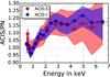 |
Fig. 2 Stacked residuals ratio, rescaled to unity at 1.1 keV. The shaded region represents the 68% confidence level from 10000 bootstrap simulations. For a detailed description see text. |
 |
Fig. 3 Stacked residuals ratios are rescaled to unity at 1.1 keV. The shaded region represents the 68% confidence level from 10000 bootstrap simulations. For a detailed description, see text. Apart from choosing EPIC-PN as the reference instrument, we also show the ACIS/MOS1, ACIS/MOS2, and MOS1/MOS2 stacked residuals. |
The situation is more problematic at lower energies. In general, the EPIC-PN vs. ACIS soft band differences are consistent with those reported in N10, but the better statistics and the systematic usage of stacked residual method in the present paper yield a more detailed view of the situation. ACIS and MOS1 vs. PN stacked residuals exhibit a systematic decrease when moving from 3 keV to 1 keV. The amplitudes are different: ~20% for ACIS/PN and ~10% for MOS1/PN. The MOS2/PN and MOS1/MOS2 ratios have smaller (~5%) and insignificant changes when moving from 3 keV to 1 keV. Especially in the (0.5−2) keV band, the MOS1/PN and MOS2/PN residuals show very similar behavior. If the shape of the effective area of PN is very accurately calibrated, the above results indicate that the ACIS (MOS1) effective area is overestimated by a factor of ~20% (~10%) at 1 keV.
The sudden increase in the stacked residual ratio at energies (1−0.5) keV by ~5% in all instruments compared to PN indicates problems with PN effective area calibration at these energies. The simplest explanation of the data is that the PN effective area is underestimated by 5% at 0.5 keV. We also detect this increase between ~1 keV and 0.5 keV in the ACIS/MOS1 and ACIS/MOS2 ratios but at a lower level (<5%).
While preparing this work, a paper by Read et al. (2014) appeared on arXiv, that employs stacked residuals of on-axis point sources. While their results are mostly consistent with ours, there is an indication of a slightly different behavior in their default analysis method (stack+fit) of the MOS2/PN case at high energies. They only see a drop in the stacked residuals for MOS2/PN, if they use the fit+stack method, as we do here. In Read et al. (2014), the authors mention “negative spectral bins that can sometimes occur in the individual source spectra” as the reason for the MOS2/PN drop in the fit+stack method. We tested this by excluding all spectra from the stacked residuals analysis, which have at least one negative bin. Since no different behavior can be detected, we conclude that negative bins do not matter in our analysis.
6.2. Temperatures
The results of the stacked residuals imply a multitude of temperature agreements and disagreements between different instruments in different energy bands (reported in Figs. 4–7 and Table A.2). In the following we compare these temperatures and evaluate the significance of temperature differences for one cluster of the sample, as well as for the whole sample.
6.2.1. Temperature comparison of individual clusters
We evaluate the temperature differences and their significances ξ by defining  (2)where TIX and TIY denote the temperatures measured with two instruments to be compared and ΔTIX and ΔTIYdenote the statistical uncertainties of the temperature for the two instruments. Here, ξ is calculated for each cluster and instrument combination individually. The ξ distributions for the detector combinations are not symmetric, but we are able to calculate the median ξ for each combination and the percentage of clusters with ξ above 3 (see Table 1). For a non-systematic temperature difference (e.g., scatter) the median should not be significantly different from zero.
As indicated by the consistent ACIS-I/PN and ACIS-S/PN stacked residuals, the ACIS-I and ACIS-S temperatures are consistent in all bands (see Figs. 4 and B.5, right). In the hard band, as indicated by the flat stack residuals, the temperatures are more consistent (most of the clusters with a ξ< 3, see Table 1). The feature of the MOS2/PN declining stacked residuals above 4.5 keV is not seen in the temperature comparison. This might be explained by the low statistical weight that this band gets in the spectral fit because of the low number of counts. In the soft band, as expected due to the systematic effect in the stacked residuals, the PN temperatures are systematically lower than those of MOS1, MOS2, and ACIS, and MOS1 and MOS2 are showing very good agreement (no cluster with ξ above 3). In the full energy band, the complex stacked residuals behavior as a function of energy results in MOS1 delivering higher temperatures than PN (due to soft band problems) and MOS2 delivering lower temperatures than MOS1 and ACIS and yielding approximate agreement with PN (see Fig. 5).
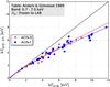 |
Fig. 4 Comparison of EPIC-PN full energy band temperatures with those obtained with ACIS-I (blue squares) and ACIS-S (red triangles). The NH is frozen to the radio value of the LAB survey. For a comparison of the resulting best-fit parameters see also Fig. B.5 and Table 2. The red and blue lines show the powerlaw best-fit function (Eq. (3)) to the ACIS-S and ACIS-I subsamples, respectively. |
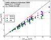 |
Fig. 5 Comparison of the full energy band temperatures obtained with the three individual XMM-Newton detectors (every detector combination has 56 objects) with those obtained with ACIS. The NH is frozen to the radio value of the LAB survey. The gray line shows the powerlaw best-fit function (Eq. (3)) to the simultaneously fitted XMM-Newton temperatures, see also Fig. 8. |
Median of the significance of temperature differences, ξ, and probability of HIFLUGCS clusters to deviate more than 3 ξ from zero for the three energy bands.
To enable a comparison with the literature, we also combined the three XMM-Newton instruments by performing a simultaneous fit (which we call “combined XMM-Newton” from now on) in the different energy bands and linking temperatures and metallicities while the normalizations are free to vary. In the combined EPIC fit, the systematic soft-band stacked residuals feature for ACIS-PN and MOS1-PN (see Fig. 3) results in lower full band EPIC temperatures (see Figs. 5–7). The ACIS-EPIC temperature differences increase with temperature in all bands. We think this is due to the spectra of the lowest temperature clusters not having enough statistics to weight the (1−3) keV band cross-calibration feature significantly.
6.2.2. Scaling relations of temperatures between different instruments
The distribution of temperature differences for any detector combination shows a Gaussian behavior in logarithmic space. We quantified this by modeling the temperatures obtained with one instrument as a powerlaw function of the values obtained with another instrument, in a given energy band, as  (3)We included intrinsic scatter ζ in the fitting process (see Table 2), which is determined by requiring
  (as done, e.g., by Maughan 2007). The intrinsic scatter is added in quadrature to the statistical uncertainty of the data to calculate the χ2 of the model. The degeneracy between the two parameters, a and b, is shown in Fig. B.4) and in Fig. 8 for the ACIS–XMM-Newton combined case. Neglecting the intrinsic scatter would result in tighter constraints of the fit parameters, hence in higher significances of temperature differences. From Fig. B.4 we conclude that for our sample the temperatures deviate for all detector combinations at least by 5σ in the full energy band, while in the soft energy band only MOS1 and MOS2 show good agreement. In the hard band no instrument combination shows deviations larger than 4.4σ. For individual clusters the average significance of differences between temperatures is smaller, as shown in Sect. 6.2.1.
We see more than a 4σ deviation between ACIS and PN even in the hard band. Looking at the stacked residual ratio for ACIS/PN (Fig. 3, top left) we see an increase in the (2−3) keV band, which might be responsible for the temperature difference in the hard band. However, this 4σ deviation is still small compared to the other bands. N10 conclude that the hard-band temperatures of ACIS and PN agree (0.88σ according to our analysis method), which was probably driven by the lower number of objects in the N10 sample. Even though N10 find consistent ACIS and PN temperatures in the hard band and we detect a more than 4σ deviation, the ellipses in the a-b-plane overlap (Fig. B.5, right panel). Since we use more than five times more objects and compare two high precision instruments here, our significance increases.
In the full band, EPIC-PN temperatures are on average 29% lower than ACIS temperatures at a cluster temperature of 10 keV (see Table 2). All detector combinations are plotted individually in Fig. B.1 for the full energy band, B.2 for the soft and B.3 for the hard energy band. Within the uncertainties, the best-fit N10 relation agrees with our full band relation (see Fig. B.5), implying persistent calibration uncertainties since 2009. Although this work deals with the Chandra CALDB 4.5.5.1, we cross-checked our results of ACIS using the new ACIS QE contamination model vN0008 included in CALDB 4.6.1. Comparing the Chandra CALDB 4.5.5.1 (default in this work) and 4.6.1, we get 1.9 % lower temperatures (2.9 % scatter) using CALDB 4.6.1 for low and medium temperature clusters. For cluster temperatures above 8 kev we find 5.4 % (4.8 % scatter) lower temperatures with CALDB 4.6.1. In a future work, we will study the effect of the new contamination model in more detail.
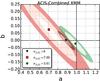 |
Fig. 8 Degeneracy of the fit parameters (see Eq. (3)) for the ACIS – Combined XMM-Newton fit. The shaded regions correspond to the 1σ, 3σ, and 5σ confidence levels. The red square represents the soft energy band, the green circle the hard, and the gray triangle the full band. Equality of temperatures is given for a = 1 and b = 0. The deviation in σ from equality is given in the legend. |
We want to mention here that we also tested the self consistency of the instruments by comparing the soft and hard band temperatures of the same instrument. However, the conclusions of these results depend strongly on the multitemperature structure of the ICM. Details are provided in Appendix C.
The combined EPIC and ACIS temperatures indicate that the clusters that are excluded because of the overly large cool core radius (see Sect. 2) do not show any systematic behavior compared to the other clusters (see Fig. 9).
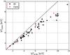 |
Fig. 9 Combined XMM-Newton versus Chandra temperature. The excluded objects (too large core radius) are marked here by red triangles. |
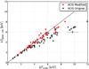 |
Fig. 10 Temperatures before and after modifying the ARF files of ACIS spectra according to the energy-dependent calibration uncertainties shown in Fig. 3. This plot shows the 53 clusters from the stacked residual ratio sample (Sect. 5.2). |
We modeled the energy dependence of the cross-calibration uncertainties by cubic spline interpolation (e.g., Press et al. 1992, Chap. 3.3). This was applied in Figs. 2, 3 and Table A.3 to the stacked residual ratios (see Sect. 6.1). These splines can be used to estimate the effect of the effective area cross-calibration uncertainties on the spectral analysis performed with a given EPIC or ACIS instrument. The effective area of a given instrument must be multiplied by the corresponding spline to obtain best-fit temperatures when assuming that the reference instrument is precisely calibrated. To convert, for example, from ACIS to EPIC-PN, one should multiply the effective area of ACIS with the energy-dependent spline values of ACIS/PN from Table A.3. The underlying assumption is, that the reason for the temperature differences between the detectors is the uncertainty in the effective area calibration. As an example, we pick the most extreme case, ACIS versus EPIC-PN: We find that indeed temperatures between ACIS and EPIC-PN (Fig. 10) are now consistent. The significance of temperature differences between ACIS and PN is now 2.7σ in the full band, while before we had a more than 8σ deviation. To enable the use of our results for calibration work, we present the spline parameters for each instrument pair in Table A.3 and we provide a tool to modify the effective area based on the splines of the stacked residual ratios7.
7. Discussion
In the previous section we have shown that systematic temperature differences exist between ACIS and the EPIC detectors. We investigate the consequences arising when our assumption of a single-temperature plasma breaks down and we have to deal with a multitemperature structure. Finally, we compare measured and independently derived hydrogen column density values and estimate the cosmological impacts of our results.
7.1. Systematics
7.1.1. Multiphase ICM
While we know the relative calibration uncertainties from the stacked residual ratios (see Sect. 6.1), we discuss here the possibility that the observed temperature differences between the instruments and detectors are not caused by calibration uncertainties but by the different effective areas and the multitemperature structure of the ICM. The role of the multiphase ICM has been discussed in detail in Mazzotta et al. (2004), Vikhlinin (2006), and Reiprich et al. (2013), among others. As shown in Reiprich et al. (2013), one can conclude from the effective areas of the instruments that Chandra is more sensitive to the harder spectra and higher temperatures than XMM-Newton, which may explain the higher temperatures if a multitemperature structure plays an important role. In the following we quantify whether this effect is significant and if a multitemperature structure is important by performing simulations. We show later that the restrictions on the two-temperature plasma cannot be fulfilled. We also show examples, where we expect a strong multiphase structure of the ICM, such as the cool core regions of CC clusters or the full (3.5′) region of clusters with a cool core larger than this size. Finally we compare the results from Chandra event files that were smoothed to the XMM-Newton resolution.
In summary, we demonstrate that none of the studied possible effects can explain the observed temperature differences.
Simulations
To test the effect on the measurements of a multitemperature plasma, we simulated a set of spectra for the different XMM-Newton detectors and for ACIS-I following the same approach presented in Reiprich et al. (2013, Sect. 4.6). To isolate the influence of multitemperature structure on best-fit temperatures, we assumed here that the instruments are perfectly calibrated. We used as test cases for the cold component three different temperatures, 0.5, 1, and 2 keV, and three different metal abundances (0.3, 0.5, and 1 times solar). The temperature of the hot component was varied from 3 to 10 keV, while the metallicity was kept fixed to 0.3 solar, a value typical of the clusters in our sample. The relative contribution of the second plasma component has been estimated by varying the emission measure ratios (from 10% to equal emission measure). We then fitted the resultant spectra with a single-temperature model and also left the metallicity free to vary. The best-fit values and the 68% errors have been taken from the distribution of 100 realizations.
We found that when the cold component is ~2 keV, the fit is always good (χ2< 1.1) independent of the amount of “cold gas” present in the cluster and of the metallicity of this gas. For cooler temperatures the amount of cold gas and its metallicity play an important role. Clearly, if the cold gas were very enriched the fit would yield a bad χ2 (>2) in almost all the cases (i.e., also with only 10% of cold gas with respect to the hot component), while for lower abundance it also depends on the amount of gas. Since in the observations we do not see such bad , we excluded all the combinations with a  . Each dataset of the simulated spectra contains 10000 counts. This is a conservative approach, since we typically have more counts in our spectra from the observed data. Owing to the higher statistics of the observed spectra with respect to the simulated ones, we would expect to find an inappropriate model (e.g., due to multitemperature structure) first in the observed data. We checked the difference in temperature between Chandra and XMM-Newton of the simulated spectra and found that the fitted temperature of the two instruments starts to be significantly different only when the second component is very cold (i.e., 0.5 keV). In Fig. 11 we only show this case. We note that to explain the observed difference between Chandra and EPIC-MOS2, an emission measure ratio (EMR) of almost 0.2 is required. We show in the next paragraphs that this is not the case. Furthermore, an EMR = 0.2 is not able to explain the observed difference between Chandra and MOS1/PN. Thus, we conclude that although a multi temperature ICM cannot be excluded, it cannot explain the observed difference in temperature between the different instruments. We also note here that a higher EMR always gives a bad χ2 that we do not observe in the real observations.
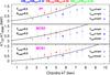 |
Fig. 11 Difference between Chandra and XMM-Newton single-temperature fits to two-temperature component mock spectra vs. the Chandra best-fit temperature. The three colors correspond to different emission measure ratios (EMR) of the cold and hot components, the symbols represent 8 different temperatures of the hot component, while its metallicity is frozen to 0.3 of the solar value and the redshift to 0.05, which corresponds to the mean HIFLUGCS redshift. The temperature and metallicity of the cold component are always fixed to 0.5 and 0.3, respectively. The black curve shows the measured temperature difference between Chandra and XMM-Newton as presented in Table 2. |
Two-temperature fits
To test the results from the simulations we selected the clusters with the highest number of counts in both XMM-Newton and Chandra: Abell 2029 has 210000 counts in Chandra and roughly 62000 counts in PN and a Chandra temperature of 8.7 keV. For both instruments, we fit a two-temperature model, fixing the temperature of the second component to 0.5 keV and the metallicity to 0.3. The temperature of the first component increased for both instruments by 3% to 4% compared to the single-temperature model. The normalization of the second component is for both instruments 1% to 5% of the first component. This is far too low to explain any temperature differences obtained by the two instruments. Also fixing the normalization of the second component to 20% of the first component increases the reduced χ2 to almost 4 for PN and >15 for ACIS.
Another good example is the cool-core cluster Abell 2142 with more than 180000 counts in both instruments and a Chandra temperature above 9 keV. This cluster has a cool core radius larger than 3.5′, so in an observation within this threshold, more than one temperature component should be present. For Chandra the normalization of a 0.5 keV component is consistent with zero. This is also true if the temperature of the cold component is frozen to 2 keV. For PN the normalization of the 0.5 keV component is below 1.5%, and for a fitted temperature of 2.7 keV of the cold component, the normalization is about 17% of the first component. From the simulations we conclude that every cold component above 2 keV cannot explain the observed difference, so we cannot find any hint of a multiphase ICM being the reason for the inconsistency of the instruments.
Multitemperature plasmas
Since galaxy clusters, in general, and especially cool-core clusters do not show only one dominant temperature, but a temperature profile, we select now regions, where a clear multiphase ICM structure is present, the cool cores of CC clusters and the whole circular region until 3.5′. Assuming that a multitemperature structure contributes significantly to the observed temperature differences, we would then expect to find significantly larger temperature differences. We do not observe this, though. We have already demonstrated in Fig. 9 that the restriction to isothermal regions does not introduce any bias, but we verify this again especially for the cool core regions. We ended up with 28 cool core region clusters and 56 clusters where we used the full circular region and compared this to the 28 clusters using the annulus region. To choose the extreme case, we only used the PN detector for XMM-Newton. As can be seen in Fig. 12, the best-fit curves do agree, and we can be sure that the multitemperature structure of clusters has no significant effect on our measurements of the instrumental differences.
Summary of the multiphase ICM tests
In this section we show that assuming the observed temperature differences are only caused by multitemperature structure of the ICM (i.e., the calibrations are perfect), we can set up restrictions on the cold plasma component (EMR ≈ 20% and kT = 0.5 keV). These restrictions were derived by fitting two simulated plasma components with a single component and requiring the observed temperature difference between detectors to be reproduced with the simulations, as well as  . Applying this to real high quality observations by fitting two plasma components we cannot recover the required emission measure of the cold component. Also we cannot see any hint of a different behavior of the temperature difference for regions with a clear multi phase structure (e.g., the cool core region), which would be expected, if the multitemperature structure is responsible for the measured temperature differences.
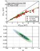 |
Fig. 12 Top: XMM-Newton/EPIC-PN versus Chandra/ACIS temperatures in the full energy band. The different colors correspond to the 3 different regions where the spectra could be extracted: The full 3.5′ circle (red squares), the cool core region (green circles), and the annulus between the two (black triangles). In the cool core region, the strongest influence of multitemperature plasma is expected. Bottom: degeneracy between the parameters a and b for the three cases shown above. The shaded regions correspond to 1σ, 3σ, and 5σ confidence levels. |
7.1.2. Temperature – abundance degeneracy
The two parameters, temperature and abundance of heavy elements, are not completely independent of each other (e.g., Gastaldello et al. 2010; Buote 2000). Since for many of our clusters, the constrained abundance also does not agree within the different instruments, it is possible that a degeneracy of the two parameters is producing inconsistent values for both of them. To make certain that this degeneracy is not the reason for the detected temperature difference, we refit the XMM-Newton data of all clusters by freezing the metallicity to the one obtained by Chandra. On average the EPIC-PN temperature increased by 0.8% compared to the best-fit temperature where the relative abundance is free to vary. For only 8 of the 56 clusters the EPIC-PN temperature increased by more than 2% (at maximum by 8.7%), but for none of these cases does the new (with frozen relative abundance to Chandra/ACIS) EPIC-PN temperature agree with Chandra/ACIS. Therefore, any inconsistency in the temperatures cannot be explained by wrongly constrained abundance, and because the temperature change described in this section is not systematic in one direction.
7.1.3. Effects of the point spread function (PSF)
The last case to discuss here is the possible scatter of the cool core emission into the annular region due to the broader XMM-Newton PSF. We used the Chandra cleaned events files and redistributed the position of all photons using a Gaussian smoothing kernel with a σ between 1″ and 70″. This scenario is different than what we simulated in Sect. 7.1.1 since we assumed there that the detectors “see” the same photon distribution, but are sensitive to different parts of the spectrum, which is more complicated than our one-component model. Then the instrument has to deal with the different photon distributions caused by the different PSFs. We tested this for four clusters, where we detect a temperature difference between XMM-Newton and Chandra and which have a strong cool core: Abell 85, Abell 133, Abell 2204, and Abell 3112. In all four cases, the temperature is very constant up to a threshold of the smoothing kernel σ. A significant drop in the temperature is detected beyond 30″, then the temperature drops constantly with increasing σ. Even if the Gaussian shape of the PSF (constant with photon energy) is not the best approximation of the real PSF behavior, we can conclude from this test that the PSF of XMM-Newton (half power diameter of 15″ on axis) is not sufficient to scatter enough emission from cooler regions.
7.2. Influence of NH and the abundance table
In this section we show the influence of the heavy elements abundance table and the hydrogen column density in the absorption model. We demonstrate that the NH constrained in a spectral fit can be compared to independently determined reference values. This comparison could help to evaluate the calibration status of a detector through the level of agreement with reverence values, but the conclusions depend on the abundance table.
The relative abundance table gives the number densities of atoms of a certain element relative to hydrogen. Most of the abundance tables are established using measurements of the solar photosphere and corona and from meteorites. It is still very common to use the (xspec default) table presented in Anders & Grevesse (1989), but we also want to test for a dependence of our results on the choice of the table by using the Asplund et al. (2009) relative abundances, which represent more recent measurements. In our analysis we are able to see a systematic effect by using this abundance table. Temperatures derived using Aspl are on average 5% higher. These higher temperatures are produced independently of the detector (ACIS and EPIC). Since this effect is much bigger than expected, we tested whether the absorption or the emission component is responsible for this change. When using the wabs instead of the phabs-model for the absorption fixes, the abundance table for the absorption model to the hard-wired abundance table from Anders & Ebihara (1982), while phabs self-consistently uses the same abundance table for absorption and emission. With the wabs model, the temperature change is then very tiny, and the results are always consistent within the errorbars. The reason for this large change in temperature by using the Aspl abundance table is given in the absorption.
The step during the spectral fitting process of accounting for the absorption of heavy elements along the line of sight is important. The absolute abundance of these metals can be traced by measuring the neutral hydrogen column density (e.g., with HI 21 cm radio measurements) and assuming relative abundances as in the solar system. A widely used HI survey is the Leiden/Argentine/Bonn (LAB) survey (Kalberla et al. 2005). The cross-calibration uncertainties of the effective area are larger at the lowest energies (Sect. 6.2), where the Galactic absorption is significant. If a) one detector had its effective area very accurately calibrated in the full energy band; and b) the emission modeling was accurate (i.e. correctly treating the possible multitemperature structure), the best-fit hydrogen column densities obtained with this instrument should be consistent with the Galactic values. Thus the free NH test could yield some information on the calibration accuracy.
We refit the full energy band EPIC-PN and ACIS spectra, allowing the temperature, metal abundance, emission measure, and the hydrogen column density to be free parameters. Using the PN detector as representative of XMM-Newton, we can conclude that Chandra systematically finds higher NH values than XMM-Newton (on average around 40%). Also compared to the LAB values, a Chandra-detected NH is systematically higher (on average 20% using AnGr), while PN detects 33% lower column densities using AnGr. Comparing the detected NH values using the Aspl abundance table with the detected column densities using AnGr reveals a strong trend toward detecting 20% to 30% higher column densities with the more recent abundance table.
The dominant element responsible for this temperature increase is oxygen, since its relative abundance value is reduced by almost 50% in the Aspl table compared to the default AnGr. This decreased relative oxygen abundance causes the detected NH values to increase, since the absolute number of oxygen atoms along the line of sight should stay constant. Conversely if the NH value is frozen, the absolute number of oxygen atoms along the line of sight is reduced by switching to the Aspl table, so the effect of absorption is lower and the temperature needs to increase to compensate for this effect.
The radio surveys measure the hydrogen column density from the HI-21 cm line. This only provides the neutral hydrogen along the line of sight, so the molecular and ionized hydrogen is not accounted for. Even if the neutral hydrogen usually contributes most to the total hydrogen, an easy method exists to account for the molecular hydrogen (for more details see Willingale et al. 2013). One can use the dust extinction E(B − V) measured in the B and V band as a tracer for the molecular hydrogen.
We therefore define the total hydrogen column density as  (4)with NH2,max = 7.2 × 1020 cm-2, Nc = 3 × 1020 cm-2, and α = 1.1 as given by Willingale et al. (2013). The relation has been calibrated using X-ray afterglows of gamma ray bursts. A webtool8 is available to calculate NH,tot for a given position using the infrared data from IRAS and COBE/DIRBE (Schlegel et al. 1998).
We compared the obtained hydrogen column density values with those derived including the molecular hydrogen Willingale et al. (2013; see Fig. 13). The median difference and the 68% scatter between the X-ray derived NH to that of Willingale et al. (2013) for ACIS and EPIC-PN are  and
and  , respectively, when using abundance table of AnGr. That Chandra constrained NH values are in better agreement with the total hydrogen column density than XMM-Newton PN could give a hint that the Chandra calibration is more reliable; however, using the Aspl abundances instead, the corresponding values are
  for ACIS and
 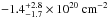 for EPIC-PN. Thus, the choice of the abundance table (i.e., the relative abundances of the elements responsible for absorption) and the scatter of the measurements make it difficult to interpret the results: The AnGr abundance table favors the ACIS derived column densities, while no conclusion can be drawn when using Aspl.
We have demonstrated that even though the most reliable calibrated instrument can be identified theoretically by comparing the constrained hydrogen column densities with references, the systematics of the abundance table that is being used, have to be taken into account.
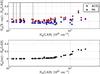 |
Fig. 13 Top: determined NH values for Chandra (red diamonds) and EPIC-PN (blue squares). Bottom: comparison of the NH,tot and the LAB hydrogen column density values for the HIFLUGCS clusters. The y-axis is in units of 1022 cm-2, and the abundance table used is AnGr. |
7.3. Cosmological impact
Galaxy clusters are excellent tools for cosmology, because they trace the dark matter and large scale structure in the Universe. In X-rays one can see the emission of the most massive visible component of galaxy clusters and measure this mass from the surface brightness profile (see, e.g., Nulsen et al. 2010). By assuming hydrostatic equilibrium the total mass can be calculated. The temperature profile of the galaxy cluster enters into this calculation as absolute value at a given radius and its logarithmic derivative (the former usually dominates, as shown in Reiprich et al. 2013, Fig. 3). To get a good handle on the cluster masses, one therefore needs accurate temperature measurements. As shown above, there is a bias depending on the X-ray instrument used. We want to quantify what effect the temperature difference between Chandra and XMM-Newton has on the cosmological parameters. Therefore we calculated the total hydrostatic masses of all HIFLUGCS clusters by establishing a temperature and density profile for each using Chandra data. The same was done to get “XMM-Newton masses” by rescaling the Chandra temperatures to “combined XMM-Newton” temperatures (see Table 2) and with that, obtaining “XMM-Newton masses”. Although it is not being used for the cosmological analysis, we present here our scaling relation for the hydrostatic masses of the different instruments for comparison reasons: 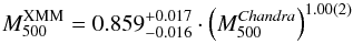 (5)(see Appendix D for more details). Since only the gradient of the density profile enters the hydrostatic equation, it is not necessary to have an accurate flux calibration for this comparison. Establishing a cluster mass function with both Chandra and XMM-Newton masses, and comparing it to the Tinker et al. (2008) halo mass function gives us constraints on the cosmological parameters ΩM and σ8. The details about this full analysis is part of a further paper on the HIFLUGCS cluster sample and is beyond the scope of the present paper, so we use a self-consistent analysis of the Chandra data, whose purpose is only to quantify the relative effect of the calibration uncertainties on the cosmological parameters.
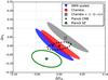 |
Fig. 14 Shift of the two cosmological parameters, ΩM and σ8, relative to the Chandra best-fit values for the X-ray analysis and relative to the Planck CMB results for the Planck analysis. The Chandra error ellipses are derived from hydrostatic masses of the HIFLUGCS clusters using Chandra temperature profiles and the Tinker halo mass function, the gray ellipse giving the results assuming a 20% hydrostatic bias. The XMM-Newton error ellipses are derived using the Chandra temperature profiles and by rescaling these profiles using Eq. (3) and Table 2. The Planck error ellipses are approximated from Planck Collaboration XX (2014). |
The resulting shift of cosmological parameters is mainly a shift toward lower ΩM when using the XMM-Newton masses. We find an 8% lower ΩM and a <1% higher σ8 for the XMM-Newton masses (see Fig. 14). Still, the 68% confidence levels in the ΩM − σ8 plane show some overlap. For precision cosmology it is necessary to quantify all systematic biases, but it seems clear that calibration differences alone cannot account for the Planck CMB primary anisotropies and Sunyaev-Zel’dovich differences (Planck Collaboration XVI 2014; Planck Collaboration XX 2014) as also shown in Fig. 14 where the relative difference between Planck SZ and Planck CMB are indicated by the unfilled ellipses. We do note that the precise shift of best-fit cosmological parameter values is expected to depend on the cluster sample under consideration. We point out that Chandra and Planck CMB overlap in this figure simply because both are arbitrarily normalized to zero for comparison reasons. This does not imply cosmological constraints from Planck CMB and Chandra galaxy clusters agree perfectly. We want to stress that the relative difference between Planck CMB and SZ best-fit values is significantly larger than the difference between Chandra and XMM-Newton derived results in the ΩM–σ8-plane.
In our analysis we also tested a hydrostatic bias,  (6)by upscaling the Chandra masses by 25% to simulate the strongest bias still allowed by the weak lensing (WL) masses determined by Israel et al. (2014a). We found a 7% higher ΩM and 6% higher σ8 for the WL masses compared to the Chandra analysis. This would correspond to a 14% difference in ΩM and 6% difference in σ8 for XMM-Newton masses compared to WL. In Fig. 14 we indicate the contours of upscaled Chandra masses in the ΩM–σ8 plane assuming (1 − b) = 0.8 by a gray square.
In the Planck SZ contours, the assumption of a uniformly varying bias in the range [ 0.7,1.0 ] enters, while the results from Israel et al. (2014a) indicate the absence of any bias and allow a maximum bias of about 20% based on the uncertainty of the intercept method. Without a marginalization of (1−b) over the range [ 0.7,1.0 ], the difference between the cosmological parameters ΩM and σ8 of the Planck primary CMB anisotropies and the SZ analyses would be even more significant, which makes it even more unlikely that the X-ray calibration uncertainties between Chandra and XMM-Newton can be responsible for this difference alone.
8. Summary and conclusions
We tested the calibration of Chandra and XMM-Newton using a large sample of very bright galaxy clusters. Analyzing the same regions, we found significant systematic differences. First, in a direct way using the stacked residual ratio method, we quantified the relative effective area uncertainties in the most extreme case (ACIS vs. EPIC-PN) by an increase of ~20% when moving in energy from 1 keV to 3 keV. Then more indirectly, but also more physically relevant, we quantified the gas temperature differences, where again the most extreme case is Chandra/ACIS and XMM-Newton/EPIC-PN at high cluster temperatures (i.e., EPIC-PN, yielding 29% lower temperatures at 10 keV in the full energy band).
We showed that physical effects like multitemperature structure cannot cause the observed temperature differences. From
-
using different energy bands for spectral fitting;
-
an energy-dependent difference of the stacked residual ratio; and
-
hydrogen column density studies,
we concluded that systematic effective area calibration uncertainties in the soft energy band (0.7−2) keV cause the observed differences. We provided fitting formulae to convert between Chandra and XMM-Newton using either effective area calibration files, temperatures, or masses (Appendix D).
To illustrate the cosmological relevance, we showed that using XMM-Newton instead of Chandra for the cluster mass function determination would result in an 8% lower ΩM and <1% different σ8. While this implies that for future high precision cluster experiments, e.g. with eROSITA (Pillepich et al. 2012; Merloni et al. 2012), this calibration needs to be improved, it also means that this systematic uncertainty alone cannot account for the Planck CMB/SZ difference.
Online material
Appendix A: Tables
63 HIFLUGCS clusters (without Abell 2244).
Best-fit temperatures and 68% confidence levels for the 4 different detectors (plus EPIC combined) in the (0.7−7) keV band.
Spline parameters (e.g., Press et al. 1992, Chap. 3.3) for the stacked residual ratios.
Appendix B: Temperature comparison
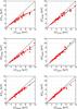 |
Fig. B.1 Best-fit temperatures of the HIFLUGCS clusters in an isothermal region for all detector combinations in the (0.7−7.0) keV energy band and with NH frozen to the radio value of the LAB survey. The parameters of the best-fit powerlaw (black line) are also shown in Fig. B.4. |
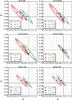 |
Fig. B.4 Fit parameter (see Eq. (3)) degeneracy for the 1, 3, and 5σ levels of the different detector combinations for the full (gray triangle), soft (red square), and hard (green circle) energy bands. Equality of temperatures for two instruments is given for a = 1 and b = 0. The deviation in σ from equality is given in the legend. |
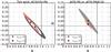 |
Fig. B.5 Left: fit parameter degeneracy for the 1, 3, and 5σ levels of ACIS – PN for the (0.7−7) keV energy band. ACIS-I (red square) and ACIS-S (black triangle) HIFLUGCS subsamples are shown versus the PN data (for all ACIS data combined, see Fig. B.4, top left panel, gray ellipse). Equality of temperatures for two instruments is given for a = 1 and b = 0. The deviation in σ from equality is given in the legend. Right: as in the left panel but only 3σ levels (gray and red ellipses) of ACIS – PN with temperatures taken from N10 (0.5−7 keV energy band, black triangle) and complete ACIS – PN of this work (0.7−7 keV energy band, red square). |
Appendix C: Self consistency test
In Sect. 6.2 we compared the best-fit temperatures of different instruments in the same energy band. In the case of purely isothermal emission and a very accurately calibrated effective area, the temperatures obtained in different energy bands of the same instrument should also be equal. By comparing temperatures of one instrument in different bands it is thus possible to quantify the absolute calibration uncertainties, if the assumption of isothermal emission is fulfilled.
In Fig. C.1 we demonstrate how self consistent the instruments are in terms of soft and hard band temperatures. We also quantify the expected deviation from equality of soft and hard band temperatures for a given two-temperature plasma.
Only for ACIS the temperature deviation (quoted σ value in the legend of Fig. C.1) is less than 3σ in comparing the soft and hard energy bands. By performing simulations similar to those shown in Sect. 7.1.1, we can quantify the expected difference between soft and hard band temperatures of the same instrument in the presence of a multitemperature structure. This is shown in Fig. C.1, where we indicate this result from simulations including a cold component with 1 keV and an EMR of 0.01, 2 keV and an EMR of 0.05, and 1 keV and an EMR of 0.05; i.e., the new symbols represent the new expected “zero points” given the multiple temperature components.
We conclude that the multitemperature structure has a strong influence on the results of this test and prevents firm conclusions on the absolute calibration. For a cold component with a temperature of ~1 keV and EMR higher than 0.01, the EPIC-PN instrument seems to agree with the simulations.
We want to emphasize that the non-detection of an effect of multitemperature ICM on comparing different instruments (as suggested in Sect. 7) is unrelated to multitemperature effects on the soft and hard band temperatures of the same instrument presented here, since the multitemperature influence may be much stronger.
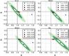 |
Fig. C.1 Fit parameter degeneracy for the 1, 3, and 5σ levels of each instrument in different energy bands. The green contours (circles) refer to the soft vs hard band. Equality of temperatures for two bands is given for a = 1 and b = 0. The deviation in σ from equality is given in the legend, as well as the expectations (blue pentagon, black square, and red diamond) for a multitemperature ICM with the parameters (temperature, emission measure ratio) of the cold component given. |
Appendix D: XMM-Newton and Chandra cross-calibration formulae
There are several methods of performing a cross-calibration between two instruments such as Chandra/ACIS and XMM-Newton/EPIC using galaxy clusters. In this work we show:
-
A correction formula for the effective area obtained using the stacked residual ratio method (Sect. 6.1 and Table A.3). For example to rescale the effective area of ACIS to give EPIC-PN consistent temperatures, one has to multiply the ACIS effective area by the spline interpolation of the ACIS/PN column of Table A.3.
-
A correction formula for the best-fit ICM temperature (Eq. (3) and Table 2); for example, for an ACIS-PN conversion in the full energy band, one has to use a = 0.836 and b = 0.016 for the parameters in Eq. (3) (with ACIS as X and PN as Y).
-
A linear relation for the hydrostatic masses (see below). The Chandra masses were calculated using the temperature and surface brightness profiles of the HIFLUGCS clusters, while the XMM-Newton masses were adopted from the rescaled Chandra temperature profiles (using Eq. (3) and Table 2).
The hydrostatic masses are shown in Fig. D.1. We found the following relation: 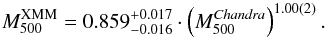 (D.1)This result agrees with the derived relations in Mahdavi et al. (2013) and is also in rough agreement with Israel et al. (2014b). In Israel et al. (2014b), the authors obtained Chandra masses by using Chandra cluster temperatures assuming temperature profiles (from a scaling relation from Reiprich et al. 2013), while the XMM-Newton masses are calculated from the rescaled temperature profiles following the temperature scaling relation presented in this work. In Mahdavi et al. (2013), the authors find similar results concerning the temperature differences and also give a conversion for the hydrostatic masses between XMM-Newton and Chandra (see Fig. D.1).
The three methods presented in this work for converting between XMM-Newton and Chandra are obviously not exactly equivalent in the context of cosmological results.
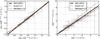 |
Fig. D.1 Comparison between Chandra and XMM-Newton in terms of hydrostatic masses in logspace (left) and realspace (right). Gray circles: Hydrostatic masses for Chandra (derived from data) and XMM-Newton (from rescaled Chandra temperature profiles). A best-fit relation (derived in logspace) is shown in black (Eq. (5)), along with the results from Israel et al. (2014b; red dashed line) and Mahdavi et al. (2013; green dotted dashed line). |
Acknowledgments
The authors would like to thank Douglas Applegate, Matteo Guainazzi and Fabio Gastaldello for helpful discussions. G.S., L.L., and T.H.R. acknowledge support by the German Research Association (DFG) through grant RE 1462/6. T.H.R. acknowledges support by the DFG through Heisenberg grant RE 1462/5. L.L. acknowledges support by the DFG through grant LO 2009/1-1 and by the German Aerospace Agency (DLR) with funds from the Ministry of Economy and Technology (BMWi) through grant 50 OR 1102. J.N. acknowledges a PUT 246 grant from Estonian Research Council.
References
- Anders, E., & Ebihara, M. 1982, Geochim. Cosmochim. Acta, 46, 2363 [NASA ADS] [CrossRef] [Google Scholar]
- Anders, E., & Grevesse, N. 1989, Geochim. Cosmochim. Acta, 53, 197 [Google Scholar]
- Asplund, M., Grevesse, N., Sauval, A. J., & Scott, P. 2009, ARA&A, 47, 481 [NASA ADS] [CrossRef] [Google Scholar]
- Balucinska-Church, M., & McCammon, D. 1992, ApJ, 400, 699 [NASA ADS] [CrossRef] [Google Scholar]
- Buote, D. A. 2000, MNRAS, 311, 176 [NASA ADS] [CrossRef] [Google Scholar]
- Donahue, M., Voit, G. M., Mahdavi, A., et al. 2014, ApJ, 794, 136 [NASA ADS] [CrossRef] [Google Scholar]
- Gastaldello, F., Ettori, S., Balestra, I., et al. 2010, A&A, 522, A34 [NASA ADS] [CrossRef] [EDP Sciences] [Google Scholar]
- Hickox, R. C., & Markevitch, M. 2006, ApJ, 645, 95 [NASA ADS] [CrossRef] [Google Scholar]
- Hudson, D. S., Mittal, R., Reiprich, T. H., et al. 2010, A&A, 513, A37 [NASA ADS] [CrossRef] [EDP Sciences] [Google Scholar]
- Israel, H., Reiprich, T. H., Erben, T., et al. 2014a, A&A, 564, A129 [NASA ADS] [CrossRef] [EDP Sciences] [Google Scholar]
- Israel, H., Schellenberger, G., Nevalainen, J., Massey, R., & Reiprich, T. 2014b [arXiv:1408.4758] [Google Scholar]
- Kalberla, P. M. W., Burton, W. B., Hartmann, D., et al. 2005, A&A, 440, 775 [NASA ADS] [CrossRef] [EDP Sciences] [Google Scholar]
- Kettula, K., Nevalainen, J., & Miller, E. D. 2013, A&A, 552, A47 [NASA ADS] [CrossRef] [EDP Sciences] [Google Scholar]
- Longinotti, A. L., de La Calle, I., Bianchi, S., Guainazzi, M., & Dovciak, M. 2008, in Rev. Mex. Astron. Astrofis. Conf. Ser., 32, 62 [Google Scholar]
- Mahdavi, A., Hoekstra, H., Babul, A., et al. 2013, ApJ, 767, 116 [NASA ADS] [CrossRef] [Google Scholar]
- Martino, R., Mazzotta, P., Bourdin, H., et al. 2014, MNRAS, 443, 2342 [NASA ADS] [CrossRef] [Google Scholar]
- Maughan, B. J. 2007, ApJ, 668, 772 [NASA ADS] [CrossRef] [Google Scholar]
- Mazzotta, P., Rasia, E., Moscardini, L., & Tormen, G. 2004, MNRAS, 354, 10 [NASA ADS] [CrossRef] [Google Scholar]
- Merloni, A., Predehl, P., Becker, W., et al. 2012 [arXiv:1209.3114v2] [Google Scholar]
- Nagai, D., Kravtsov, A. V., & Vikhlinin, A. 2007, ApJ, 668, 1 [NASA ADS] [CrossRef] [Google Scholar]
- Nevalainen, J., David, L., & Guainazzi, M. 2010, A&A, 523, A22 [NASA ADS] [CrossRef] [EDP Sciences] [Google Scholar]
- Nulsen, P. E. J., Powell, S. L., & Vikhlinin, A. 2010, ApJ, 722, 55 [NASA ADS] [CrossRef] [Google Scholar]
- Pillepich, A., Porciani, C., & Reiprich, T. H. 2012, MNRAS, 422, 44 [NASA ADS] [CrossRef] [Google Scholar]
- Planck Collaboration XVI. 2014, A&A, 571, A16 [NASA ADS] [CrossRef] [EDP Sciences] [Google Scholar]
- Planck Collaboration XX. 2014, A&A, 571, A20 [NASA ADS] [CrossRef] [EDP Sciences] [Google Scholar]
- Press, W. H., Teukolsky, S. A., Vetterling, W. T., & Flannery, B. P. 1992, Numerical recipes in C. The art of scientific computing [Google Scholar]
- Read, A. M., Guainazzi, M., & Sembay, S. 2014, A&A, 564, A75 [NASA ADS] [CrossRef] [EDP Sciences] [Google Scholar]
- Reiprich, T. H., & Böhringer, H. 2002, ApJ, 567, 716 [NASA ADS] [CrossRef] [Google Scholar]
- Reiprich, T. H., Basu, K., Ettori, S., et al. 2013, Space Sci. Rev., 177, 195 [NASA ADS] [CrossRef] [EDP Sciences] [Google Scholar]
- Rozo, E., Bartlett, J. G., Evrard, A. E., & Rykoff, E. S. 2014, MNRAS, 438, 78 [NASA ADS] [CrossRef] [Google Scholar]
- Schlegel, D. J., Finkbeiner, D. P., & Davis, M. 1998, ApJ, 500, 525 [NASA ADS] [CrossRef] [Google Scholar]
- Smith, R. K., Brickhouse, N. S., Liedahl, D. A., & Raymond, J. C. 2001, ApJ, 556, L91 [NASA ADS] [CrossRef] [Google Scholar]
- Snowden, S. L., Collier, M. R., & Kuntz, K. D. 2004, ApJ, 610, 1182 [NASA ADS] [CrossRef] [Google Scholar]
- Tinker, J., Kravtsov, A. V., Klypin, A., et al. 2008, ApJ, 688, 709 [NASA ADS] [CrossRef] [Google Scholar]
- Vikhlinin, A. 2006, ApJ, 640, 710 [NASA ADS] [CrossRef] [Google Scholar]
- von der Linden, A., Mantz, A., Allen, S. W., et al. 2014, MNRAS, 443, 1973 [NASA ADS] [CrossRef] [Google Scholar]
- Wargelin, B. J., Markevitch, M., Juda, M., et al. 2004, ApJ, 607, 596 [Google Scholar]
- Willingale, R., Starling, R. L. C., Beardmore, A. P., Tanvir, N. R., & O’Brien, P. T. 2013, MNRAS, 431, 394 [NASA ADS] [CrossRef] [Google Scholar]
- Zhang, Y.-Y., Andernach, H., Caretta, C. A., et al. 2011, A&A, 526, A105 [NASA ADS] [CrossRef] [EDP Sciences] [Google Scholar]
All Tables
Median of the significance of temperature differences, ξ, and probability of HIFLUGCS clusters to deviate more than 3 ξ from zero for the three energy bands.
Best-fit temperatures and 68% confidence levels for the 4 different detectors (plus EPIC combined) in the (0.7−7) keV band.
Spline parameters (e.g., Press et al. 1992, Chap. 3.3) for the stacked residual ratios.
All Figures
|
Fig. 1 Relative temperature difference resulting from raising the background level by 10% for energies below 2 keV. |
| In the text | |
|
Fig. 2 Stacked residuals ratio, rescaled to unity at 1.1 keV. The shaded region represents the 68% confidence level from 10000 bootstrap simulations. For a detailed description see text. |
| In the text | |
|
Fig. 3 Stacked residuals ratios are rescaled to unity at 1.1 keV. The shaded region represents the 68% confidence level from 10000 bootstrap simulations. For a detailed description, see text. Apart from choosing EPIC-PN as the reference instrument, we also show the ACIS/MOS1, ACIS/MOS2, and MOS1/MOS2 stacked residuals. |
| In the text | |
|
Fig. 4 Comparison of EPIC-PN full energy band temperatures with those obtained with ACIS-I (blue squares) and ACIS-S (red triangles). The NH is frozen to the radio value of the LAB survey. For a comparison of the resulting best-fit parameters see also Fig. B.5 and Table 2. The red and blue lines show the powerlaw best-fit function (Eq. (3)) to the ACIS-S and ACIS-I subsamples, respectively. |
| In the text | |
|
Fig. 5 Comparison of the full energy band temperatures obtained with the three individual XMM-Newton detectors (every detector combination has 56 objects) with those obtained with ACIS. The NH is frozen to the radio value of the LAB survey. The gray line shows the powerlaw best-fit function (Eq. (3)) to the simultaneously fitted XMM-Newton temperatures, see also Fig. 8. |
| In the text | |
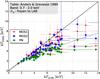 |
Fig. 6 Same as Fig. 5, except in the soft energy band (0.7−2) keV. |
| In the text | |
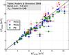 |
Fig. 7 Same as Fig. 5, except in the hard energy band (2−7) keV. |
| In the text | |
|
Fig. 8 Degeneracy of the fit parameters (see Eq. (3)) for the ACIS – Combined XMM-Newton fit. The shaded regions correspond to the 1σ, 3σ, and 5σ confidence levels. The red square represents the soft energy band, the green circle the hard, and the gray triangle the full band. Equality of temperatures is given for a = 1 and b = 0. The deviation in σ from equality is given in the legend. |
| In the text | |
|
Fig. 9 Combined XMM-Newton versus Chandra temperature. The excluded objects (too large core radius) are marked here by red triangles. |
| In the text | |
|
Fig. 10 Temperatures before and after modifying the ARF files of ACIS spectra according to the energy-dependent calibration uncertainties shown in Fig. 3. This plot shows the 53 clusters from the stacked residual ratio sample (Sect. 5.2). |
| In the text | |
|
Fig. 11 Difference between Chandra and XMM-Newton single-temperature fits to two-temperature component mock spectra vs. the Chandra best-fit temperature. The three colors correspond to different emission measure ratios (EMR) of the cold and hot components, the symbols represent 8 different temperatures of the hot component, while its metallicity is frozen to 0.3 of the solar value and the redshift to 0.05, which corresponds to the mean HIFLUGCS redshift. The temperature and metallicity of the cold component are always fixed to 0.5 and 0.3, respectively. The black curve shows the measured temperature difference between Chandra and XMM-Newton as presented in Table 2. |
| In the text | |
|
Fig. 12 Top: XMM-Newton/EPIC-PN versus Chandra/ACIS temperatures in the full energy band. The different colors correspond to the 3 different regions where the spectra could be extracted: The full 3.5′ circle (red squares), the cool core region (green circles), and the annulus between the two (black triangles). In the cool core region, the strongest influence of multitemperature plasma is expected. Bottom: degeneracy between the parameters a and b for the three cases shown above. The shaded regions correspond to 1σ, 3σ, and 5σ confidence levels. |
| In the text | |
|
Fig. 13 Top: determined NH values for Chandra (red diamonds) and EPIC-PN (blue squares). Bottom: comparison of the NH,tot and the LAB hydrogen column density values for the HIFLUGCS clusters. The y-axis is in units of 1022 cm-2, and the abundance table used is AnGr. |
| In the text | |
|
Fig. 14 Shift of the two cosmological parameters, ΩM and σ8, relative to the Chandra best-fit values for the X-ray analysis and relative to the Planck CMB results for the Planck analysis. The Chandra error ellipses are derived from hydrostatic masses of the HIFLUGCS clusters using Chandra temperature profiles and the Tinker halo mass function, the gray ellipse giving the results assuming a 20% hydrostatic bias. The XMM-Newton error ellipses are derived using the Chandra temperature profiles and by rescaling these profiles using Eq. (3) and Table 2. The Planck error ellipses are approximated from Planck Collaboration XX (2014). |
| In the text | |
|
Fig. B.1 Best-fit temperatures of the HIFLUGCS clusters in an isothermal region for all detector combinations in the (0.7−7.0) keV energy band and with NH frozen to the radio value of the LAB survey. The parameters of the best-fit powerlaw (black line) are also shown in Fig. B.4. |
| In the text | |
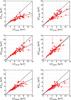 |
Fig. B.2 Same as Fig. B.1 but for the (0.7−2.0) keV band. |
| In the text | |
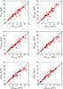 |
Fig. B.3 Same as Fig. B.1 but for the (2.0−7.0) keV band. |
| In the text | |
|
Fig. B.4 Fit parameter (see Eq. (3)) degeneracy for the 1, 3, and 5σ levels of the different detector combinations for the full (gray triangle), soft (red square), and hard (green circle) energy bands. Equality of temperatures for two instruments is given for a = 1 and b = 0. The deviation in σ from equality is given in the legend. |
| In the text | |
|
Fig. B.5 Left: fit parameter degeneracy for the 1, 3, and 5σ levels of ACIS – PN for the (0.7−7) keV energy band. ACIS-I (red square) and ACIS-S (black triangle) HIFLUGCS subsamples are shown versus the PN data (for all ACIS data combined, see Fig. B.4, top left panel, gray ellipse). Equality of temperatures for two instruments is given for a = 1 and b = 0. The deviation in σ from equality is given in the legend. Right: as in the left panel but only 3σ levels (gray and red ellipses) of ACIS – PN with temperatures taken from N10 (0.5−7 keV energy band, black triangle) and complete ACIS – PN of this work (0.7−7 keV energy band, red square). |
| In the text | |
|
Fig. C.1 Fit parameter degeneracy for the 1, 3, and 5σ levels of each instrument in different energy bands. The green contours (circles) refer to the soft vs hard band. Equality of temperatures for two bands is given for a = 1 and b = 0. The deviation in σ from equality is given in the legend, as well as the expectations (blue pentagon, black square, and red diamond) for a multitemperature ICM with the parameters (temperature, emission measure ratio) of the cold component given. |
| In the text | |
|
Fig. D.1 Comparison between Chandra and XMM-Newton in terms of hydrostatic masses in logspace (left) and realspace (right). Gray circles: Hydrostatic masses for Chandra (derived from data) and XMM-Newton (from rescaled Chandra temperature profiles). A best-fit relation (derived in logspace) is shown in black (Eq. (5)), along with the results from Israel et al. (2014b; red dashed line) and Mahdavi et al. (2013; green dotted dashed line). |
| In the text | |
Current usage metrics show cumulative count of Article Views (full-text article views including HTML views, PDF and ePub downloads, according to the available data) and Abstracts Views on Vision4Press platform.
Data correspond to usage on the plateform after 2015. The current usage metrics is available 48-96 hours after online publication and is updated daily on week days.
Initial download of the metrics may take a while.