© ESO, 2015

1. Introduction

Despite the apparent ease with which nature is forming planets, current models of planet and even planetesimal formation have problems growing large bodies within the typical gas disk lifetime of ~10⁶ years (Haisch et al. 2001). The process of planetesimal formation is a complex one, with many different processes acting on a variety of lengths and timescales (see Testi et al. 2014; and Johansen et al. 2014, for recent reviews).

The first step towards planetesimal formation is the coagulation of small dust aggregates that stick together through surface forces. As aggregates collide and stick to form larger aggregates, these aggregates have to overcome several hurdles on their way to becoming planetesimals. One important obstacle faced by a growing dust aggregate is the radial drift barrier (Whipple 1972; Weidenschilling 1977). When aggregates grow to a certain size (about a meter at 1 AU and a millimeter at 100 AU, assuming compact particles) they will decouple from the pressure-supported gas disk, and start to lose angular momentum to the gas around them. As a result, said particles will drift inward.

Even before radial drift becomes problematic, the coagulation of aggregates can be frustrated by catastrophic fragmentation or bouncing (Blum & Wurm 2008; Güttler et al. 2010; Zsom et al. 2010), which prevents colliding aggregates from gaining mass. These problems are alleviated somewhat by including velocity distributions between pairs of particles (Windmark et al. 2012; Garaud et al. 2013) in combination with mass transfer in high-velocity collisions (Wurm et al. 2005; Kothe et al. 2010), though these solutions require the presence of relatively compact targets.

Recently, it has been proposed that icy aggregates, if they can manage to stay very porous, suffer less from these barriers, and might be able to form planetesimals locally and on relatively short timescales (Okuzumi et al. 2012; Kataoka et al. 2013a). Very porous, or fluffy, aggregates are less likely to bounce (Wada et al. 2011; Seizinger & Kley 2013), and icy particles have much higher fragmentation threshold velocities than refractory ones (Dominik & Tielens 1997; Wada et al. 2013), but perhaps most surprising was the finding that porous aggregates can outgrow the radial drift barrier, by growing very rapidly as a result of their enhanced collisional cross section (Okuzumi et al. 2012). However, Okuzumi et al. (2012) assumed perfect sticking between colliding aggregates, neglecting possible mass-loss in aggregate-aggregate collisions.

We study the effects of the existence of an erosive regime for icy aggregates, where collisions at low mass ratios will produce erosive fragments at velocities below a critical erosion threshold velocity (Schräpler & Blum 2011; Seizinger et al. 2013; Gundlach & Blum 2014). Our goal is to quantify how erosion influences the direct formation of planetesimals through coagulation. To this end, we develop a local Monte Carlo coagulation code, capable of simulating the vertically-integrated dust population, tracing both the evolution of the mass and the porosity of the entire mass distribution self-consistently. Section 2 describes the models we use for the protoplanetary disk and the dust aggregates. In Sect. 3, we present the numerical method, which is based on the work of Ormel & Spaans (2008). Then, we test our model against the results of Okuzumi et al. (2012) (Sect. 4.1.1), after which we expand the model to include compaction from gas pressure and self-gravity according to Kataoka et al. (2013a) (Sect. 4.1.2), and erosive collisions (Sect. 4.2). In Sect. 5, we compare the results to a simple semi-analytical model, and describe which processes can limit coagulation in different parts of protoplanetary disks. Discussion of the results and implications takes place in Sect. 6, and conclusions are presented in Sect. 7.

2. Disk and dust models

The disk model and collisional compaction prescription are based on Okuzumi et al. (2012), to which we add non-collisional compaction processes (Sect. 2.4.2) and a model for erosive collisions (Sects. 2.3.2 and 2.3.3).

2.1. Disk structure

The disk model used in this work is based on the minimum-mass solar nebula (MMSN) of Hayashi (1981). The evolution of the gas surface density and temperature as a function of radial distance R from the Sun-like central star are given as 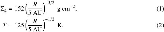$\begin{array}{ccc}{\mathrm{\Sigma }}_{\mathrm{g}}& \mathrm{=}& \mathrm{152}{\left(\frac{\mathit{R}}{\mathrm{5}\mathrm{AU}}\right)}^{\mathrm{-}\mathrm{3}\mathit{/}\mathrm{2}}\mathrm{g}\mathrm{c}{\mathrm{m}}^{-2}\mathit{,}\\ \mathit{T}& \mathrm{=}& \mathrm{125}{\left(\frac{\mathit{R}}{\mathrm{5}\mathrm{AU}}\right)}^{\mathrm{-}\mathrm{1}\mathit{/}\mathrm{2}}\mathrm{K}\mathit{.}\end{array}$The gas sound speed is given by 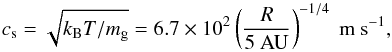${\mathit{c}}_{\mathrm{s}}\mathrm{=}\sqrt{{\mathit{k}}_{\mathrm{B}}\mathit{T}\mathit{/}{\mathit{m}}_{\mathrm{g}}}\mathrm{=}\mathrm{6.7}\mathrm{\times }{\mathrm{10}}^{\mathrm{2}}{\left(\frac{\mathit{R}}{\mathrm{5}\mathrm{AU}}\right)}^{\mathrm{-}\mathrm{1}\mathit{/}\mathrm{4}}\mathrm{m}{\mathrm{s}}^{-1}\mathit{,}$(3)with k_B the Boltzmann constant and m_g = 3.9 × 10^-24 g the mean molecular weight. The Kepler frequency equals 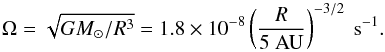$\mathrm{\Omega }\mathrm{=}\sqrt{\mathit{G}{\mathit{M}}_{\mathrm{\odot }}\mathit{/}{\mathit{R}}^{\mathrm{3}}}\mathrm{=}\mathrm{1.8}\mathrm{\times }{\mathrm{10}}^{-8}{\left(\frac{\mathit{R}}{\mathrm{5}\mathrm{AU}}\right)}^{\mathrm{-}\mathrm{3}\mathit{/}\mathrm{2}}{\mathrm{s}}^{-1}\mathit{.}$(4)Assuming an isothermal column, the gas density drops with increasing distance from the midplane z according to 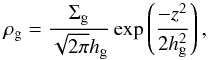${\mathit{\rho }}_{\mathrm{g}}\mathrm{=}\frac{{\mathrm{\Sigma }}_{\mathrm{g}}}{\sqrt{\mathrm{2}\mathit{\pi }}{\mathit{h}}_{\mathrm{g}}}\exp \left(\frac{\mathrm{-}{\mathit{z}}^{\mathrm{2}}}{\mathrm{2}{\mathit{h}}_{\mathrm{g}}^{\mathrm{2}}}\right)\mathit{,}$(5)with the relative vertical scale height of the gas h_g/R = 0.05(R/ 5 AU)^1/4. The turbulent viscosity is parametrized as ${\mathit{\nu }}_{\mathrm{turb}}\mathrm{=}\mathit{\alpha }{\mathit{c}}_{\mathrm{s}}^{\mathrm{2}}\mathit{/}\mathrm{\Omega }$ following Shakura & Sunyaev (1973), and α is assumed to be constant in both the radial and the vertical direction. The eddie turn-over time of the largest eddies equals t_L = Ω^-1.

In our local model, the surface density of the dust is related to the gas surface density through Σ_d/ Σ_g = 10^-2, but the vertical distribution of dust depends on its aerodynamic properties. The dust is described by a Gaussian, with the dust scale height h_d set by the stopping time t_s of the dust particle through (Youdin & Lithwick 2007) 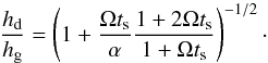$\frac{{\mathit{h}}_{\mathrm{d}}}{{\mathit{h}}_{\mathrm{g}}}\mathrm{=}{\left(\mathrm{1}\mathrm{+}\frac{\mathrm{\Omega }{\mathit{t}}_{\mathrm{s}}}{\mathit{\alpha }}\frac{\mathrm{1}\mathrm{+}\mathrm{2}\mathrm{\Omega }{\mathit{t}}_{\mathrm{s}}}{\mathrm{1}\mathrm{+}\mathrm{\Omega }{\mathit{t}}_{\mathrm{s}}}\right)}^{\mathrm{-}\mathrm{1}\mathit{/}\mathrm{2}}\mathrm{·}$(6)Thus, settling becomes important when a dust particle reaches Ωt_s ~ α.

2.2. Dust properties

Initially, all dust particles are assumed to be spherical (sub)micron-size monomers. In time, these monomers coagulate through collisions, and aggregates of considerable mass can be formed. Any aggregate is described by two parameters: the mass m, and the filling factor φ. Since aggregates are made up of monomers the mass can be written as m = Nm₀, with N the number of monomers and m₀ the monomer mass. Following Okuzumi et al. (2012), we define the internal density of an aggregate as ρ_int = m/V, with V = (4/3)πa³ the volume of the aggregate, and a its radius. An aggregate’s radius is defined as $\mathit{a}\mathrm{=}\mathrm{[}\mathrm{5}\mathit{/}\mathrm{(}\mathrm{3}\mathit{N}\mathrm{\left)}{\sum }_{\mathit{k}\hspace{0.17em}\mathrm{=}\hspace{0.17em}\mathrm{1}}^{\mathit{N}}\mathrm{\right(}{{r}}_{\mathit{k}}\mathrm{-}{{r}}_{\mathrm{CM}}{\mathrm{)}}^{\mathrm{2}}{\mathrm{]}}^{\mathrm{1}\mathit{/}\mathrm{2}}$, with r_k the position of monomer k and r_CM the position of the aggregate’s center of mass (Mukai et al. 1992; Suyama et al. 2008; Okuzumi et al. 2009). By definition, monomers have an internal density of ρ_int = m₀/V₀ = ρ₀, while aggregates can have ρ_int ≪ ρ₀. Since we are interested in region beyond the snow-line, we focus here on monomers composed of mostly ice, and use a density of ρ₀ = 1.4 g cm^-3. For the monomer radius we use a₀ = 0.1 μm. We define the filling factor as $\mathit{\phi }\mathrm{\equiv }\frac{{\mathit{\rho }}_{\mathrm{int}}}{{\mathit{\rho }}_{\mathrm{0}}}\mathit{,}$(7)as a measure for the internal density.

In the rest of this section, we describe the main ingredients for the simulations presented in Sect. 3. These are: the relative velocities between aggregates, the equations governing the evolution of ρ_int through mutual collisions as well as gas ram pressure and self-gravity, and models for the destructive processes of erosion and fragmentation.

2.2.1. Relative velocities

We take into account relative velocities arising from Brownian motion, turbulence, settling, radial drift and azimuthal drift (see Sect. 2.3.2 of Okuzumi et al. 2012). The relative contribution of the velocity components depends strongly on the size and aerodynamic properties of the dust grains in question. More specifically, the relative velocity is a function of the stopping times of the particles. Depending on the size of the particle, the stopping time is set either by Epstein or Stokes drag 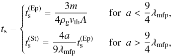${\mathit{t}}_{\mathrm{s}}\mathrm{=}\{\begin{array}{c}\\ & \mathrm{for}\mathit{a}\mathit{<}\frac{\mathrm{9}}{\mathrm{4}}{\mathit{\lambda }}_{\mathrm{mfp}}\mathit{,}\\ & \mathrm{for}\mathit{a}\mathit{>}\frac{\mathrm{9}}{\mathrm{4}}{\mathit{\lambda }}_{\mathrm{mfp}}\mathit{,}\end{array}$(8)where ${\mathit{v}}_{\mathrm{th}}\mathrm{=}\sqrt{\mathrm{8}\mathit{/}\mathit{\pi }}{\mathit{c}}_{\mathrm{s}}$ is the mean thermal velocity of the gas molecules, and λ_mfp = m_g/ (σ_molρ_g) is the gas molecule mean free path. Taking σ_mol = 2 × 10^-15 cm², we obtain λ_mfp = 120(R/ 5 AU)^11/4 cm at the disk midplane. In Eq. (8), a = a₀(V/V₀)^1/3 refers to the dust particle radius, while A is the projected cross section of the particle averaged over all orientations, which can be obtained using the formulation of Okuzumi et al. (2009).

The above equation is accurate when the particle Reynolds number Re_p = 4av_dg/ (v_thλ_mfp) < 1, with v_dg the relative velocity between the gas and the dust particle. The Reynolds number can become large when aggregates grow very big or their velocity relative to the gas is very large. In general, the stopping time can be written as 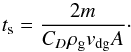${\mathit{t}}_{\mathrm{s}}\mathrm{=}\frac{\mathrm{2}\mathit{m}}{{\mathit{C}}_{\mathit{D}}{\mathit{\rho }}_{\mathrm{g}}{\mathit{v}}_{\mathrm{dg}}\mathit{A}}\mathrm{·}$(9)In the Stokes regime the drag coefficient equals C_D = 24/Re_p, and the stopping time becomes independent of v_dg. However, for larger Reynolds number the stopping time becomes a function of the velocity relative to the gas. This regime is called the Newton drag regime. Since the relative velocity depends in turn on the stopping time, we have to iterate to find the corresponding stopping time. Following Weidenschilling (1977), we use 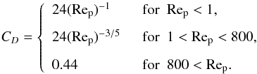${\mathit{C}}_{\mathit{D}}\mathrm{=}\{\begin{array}{c}\\ & \mathrm{for}\mathrm{R}{\mathrm{e}}_{\mathrm{p}}\mathit{<}\mathrm{1}\mathit{,}\\ & \mathrm{for}\mathrm{1}\mathit{<}\mathrm{R}{\mathrm{e}}_{\mathrm{p}}\mathit{<}\mathrm{800}\mathit{,}\\ & \mathrm{for}\mathrm{800}\mathit{<}\mathrm{R}{\mathrm{e}}_{\mathrm{p}}\mathit{.}\end{array}$(10)Figure 1 shows Stokes numbers (Ωt_s) for different particles in the midplane of a MMSN disk at 5 AU. Different lines show compact particles (red), porous aggregates with constant φ = 10⁴ (yellow), and aggregates with a constant fractal dimension of 2.5 (green). For the solid lines, all drag regimes (Epstein, Stokes and Newton) have been taken into account, while the dashed lines indicate the results using only Epstein and Stokes drag, i.e., assuming that Re_p< 1. Focussing on the D_f = 2.5 aggregates, we can clearly distinguish the different drag regimes. The smallest particles are in the Epstein regime, and switch to the Stokes regime around Ωt_s = 10^-3. Then, at a mass of m/m₀ ~ 10²¹, the Reynolds number exceeds unity and we enter the second regime of Eq. (10). We note that this transition occurs before Ωt_s = 1. The most massive particles, m/m₀> 10²⁶ are in the regime where C_D = 0.44. Compact particles on the other hand, reach Ωt_s = 1 while still in the Epstein drag regime.

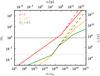Fig. 1 Particle Stokes numbers as a function of mass, in the midplane of an MMSN disk at 5 AU. Different lines show compact particles (red), porous aggregates with constant φ = 104 (yellow), and aggregates with a constant fractal dimension of 2.5 (green). For the solid lines, all drag regimes (Epstein, Stokes and Newton) have been taken into account, while the dashed lines indicate the results using only Epstein and Stokes drag. Horizontal lines indicate Ωts = 1 (where drift is fastest) and Ωts = α = 10-3 (where particles start to settle to the midplane).

The turbulence-induced relative velocity between two particles with stopping times t_s,1 and t_s,2 ≤ t_s,1 has three regimes (Ormel & Cuzzi 2007) 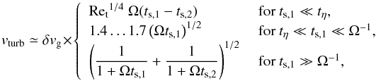${\mathit{v}}_{\mathrm{turb}}\mathrm{\simeq }\mathit{\delta }{\mathit{v}}_{\mathrm{g}}\mathrm{\times }\{\begin{array}{c}\\ & \mathrm{for}{\mathit{t}}_{\mathrm{s}\mathit{,}\mathrm{1}}\mathrm{\ll }{\mathit{t}}_{\mathit{\eta }}\mathit{,}\\ & \mathrm{for}{\mathit{t}}_{\mathit{\eta }}\mathrm{\ll }{\mathit{t}}_{\mathrm{s}\mathit{,}\mathrm{1}}\mathrm{\ll }{\mathrm{\Omega }}^{-1}\mathit{,}\\ & \mathrm{for}{\mathit{t}}_{\mathrm{s}\mathit{,}\mathrm{1}}\mathrm{\gg }{\mathrm{\Omega }}^{-1}\mathit{,}\end{array}$(11)where δv_g = α^1/2c_s is the mean random velocity of the largest turbulent eddies, and t_η = Re_t^1/2t_L is the turn-over time of the smallest eddies. The turbulence Reynolds number is given by $\mathrm{R}{\mathrm{e}}_{\mathrm{t}}\mathrm{=}\mathit{\alpha }{\mathit{c}}_{\mathrm{s}}^{\mathrm{2}}\mathit{/}\mathrm{\left(}\mathrm{\Omega }{\mathit{\nu }}_{\mathrm{mol}}\mathrm{\right)}$, with the molecular viscosity ν_mol = v_thλ_mfp/ 2. We will refer to the first two cases of Eq. (11) as the first and second turbulence regimes. Relative velocities between similar particles (similar in the sense that they have comparable stopping times) are very small¹ in the first turbulence regime because of the (t_s,1 − t_s,2) term, but considerably larger in the second regime.

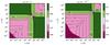Fig. 2 Relative velocities between compact (left) or very porous (right) particles with masses mi and mj at the midplane of an MMSN-disk at 5 AU with α = 10-3. The masses range from single monomers to aggregates containing 1032 monomers. The contours give relative velocities in m s-1, and the colors indicate the dominating source for the relative velocity: Brownian motion (BrM), turbulence (Trb), settling (Set), radial drift (Rad), or azimuthal drift (Azi). Epstein, Stokes, and Newton drag regimes have been taken into account.

Figure 2 shows the midplane relative velocity in m s^-1 (contours), and its dominant source (color), for a range of combinations of masses m_i and m_j. The velocities have been calculated for the disk properties of Sect. 2.1, at 5 AU, and assuming a turbulence α = 10^-3. The left plot corresponds to two compact particles (ρ_int = ρ₀), and the right plot to two very porous ones (ρ_int = 10^-4ρ₀). The general picture is the same for all porosities: Brownian motion dominates the relative velocity at the smallest sizes, followed by turbulence for larger particles, and systematic drift for bodies that have Ωt_s ~ 1. However, the masses at which various transitions occur can vary by several orders of magnitude depending on the particle porosity. For this particular location and turbulence strength, there is no combination of particle masses whose relative velocity is dominated by differential settling.

2.3. Collisional outcomes

A collision between porous aggregates can have a number of outcomes, ranging from perfect sticking to catastrophic fragmentation. For silicates, Blum & Wurm (2008) and Güttler et al. (2010) offer reviews of the various outcomes as observed in laboratory experiments. For porous ices, experimental investigations are scarce, and we have to turn to numerical simulations when predicting the outcome (e.g., Dominik & Tielens 1997; Wada et al. 2007; Suyama et al. 2008; Wada et al. 2009).

In general, a collision can result in sticking, erosion, or fragmentation, depending on the relative velocity and the mass ratio R^(m) ≡ m_i/m_j ≤ 1 of the colliding bodies. Collisions between particles with comparable masses result in catastrophic fragmentation if they collide above the fragmentation velocity (Sect. 2.3.1). When colliding bodies have a mass ratio R^(m) ≪ 1, catastrophic fragmentation of the larger body is difficult, but the collision can result in erosion if the velocity is high enough. The transition from erosion to the fragmentation regime occurs at a mass ratio ${\mathit{R}}_{\mathrm{crit}}^{\mathrm{\left(}\mathit{m}\mathrm{\right)}}$, specified in Sect. 2.3.3. In an erosive event, the larger body will lose mass. From Fig. 2 it is clear that the highest velocities are reached between particles with very different masses, and thus erosion might very well be a common collisional outcome. We discuss erosion in more detail in Sect. 2.3.2. We should note at this point that we do not consider bouncing collisions. For relatively compact silicate particles, bouncing is frequently observed in the laboratory (e.g., Güttler et al. 2010), and indeed can halt growth in protoplanetary disks (Zsom et al. 2010). However, in porous aggregates, the average coordination number (the number of contacts per monomer) is much lower than in compact ones. As a result, collision energy is more easily dissipated, and it is safe to neglect bouncing (Wada et al. 2011; Seizinger & Kley 2013).

2.3.1. Catastrophic fragmentation

For collisions between roughly equal icy aggregates (mass ratio R^(m) ≥ 1/64), Wada et al. (2013) find a critical fragmentation velocity of 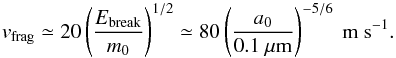${\mathit{v}}_{\mathrm{frag}}\mathrm{\simeq }\mathrm{20}{\left(\frac{{\mathit{E}}_{\mathrm{break}}}{{\mathit{m}}_{\mathrm{0}}}\right)}^{\mathrm{1}\mathit{/}\mathrm{2}}\mathrm{\simeq }\mathrm{80}{\left(\frac{{\mathit{a}}_{\mathrm{0}}}{\mathrm{0.1}\mathit{\mu }\mathrm{m}}\right)}^{\mathrm{-}\mathrm{5}\mathit{/}\mathrm{6}}\mathrm{m}{\mathrm{s}}^{-1}\mathit{.}$(12)The quantity E_break represents the energy needed to break a single mononer-monomer contact (Dominik & Tielens 1997). Collisions below this critical velocity result in sticking, while collisions at or above v_frag result in fragmentation of the collision partners.

2.3.2. The case for erosion

The relative velocity between similar-sized aggregates will generally not reach the fragmentation velocity (Eq. (12)) behind the snow line in a protoplanetary disk, especially not if the turbulence is weak. However, relative velocities between particles with very different masses can be much larger than velocities between similar particles, especially when radial and azimuthal drift are important (Fig. 2). In this paper, we study the effects of an erosive regime, where collisions at low mass ratios will produce erosive fragments at velocities below a critical erosion threshold velocity v_eros ≲ v_frag. Here, we briefly revisit numerical and experimental studies of erosion, before outlining the erosion model used in this work. The process of erosion can be described by two main quantities: the erosion threshold velocity, v_eros, above which erosion takes place, and the (normalized) erosion efficiency, ϵ_eros, that indicates how much mass is eroded in units of projectile mass.

For silicate particles, Güttler et al. (2010) summarize a number of experimental investigations and describe a threshold velocity of a few m s^-1, and an erosion efficiency that increases roughly linearly with collision velocity. Similar trends were observed by Schräpler & Blum (2011), who found an erosion threshold velocity of a few m s^-1 using micron-size silicate projectiles. We note that the threshold velocity is comparable to the monomer sticking velocity of micron-size silicate particles (Poppe et al. 2000). In the experiments of Schräpler & Blum (2011), the erosion efficiency also increased with impact velocity, reaching ~10 for the highest velocity of 60 m s^-1 (their Fig. 5). Seizinger et al. (2013) used molecular dynamics simulations, based on a new viscoelastic model (Krijt et al. 2013), to reproduce the experimental results. In addition, Seizinger et al. (2013) studied the variation on the threshold velocity and erosion efficiency with projectile mass, showing a trend of decreasing erosion threshold with decreasing mass ratio (e.g., their Fig. 11). For monomer projectiles, the threshold velocity equals the monomer-monomer sticking velocity ${\mathit{v}}_{\mathrm{s}}\mathrm{\simeq }\sqrt{{\mathit{E}}_{\mathrm{break}}\mathit{/}{\mathit{m}}_{\mathrm{0}}}$, after which it increased linearly with velocity to eventually flatten off around 10 m s^-1. This flattening off indicates the onset of catastrophic fragmentation, and occurs at a mass ratio of ~10^-2.

For ice particles, Gundlach & Blum (2014) present recent experimental results on the sticking and erosion threshold of (sub)micron-size particles. For a projectile distribution between 0.2−6 μm (with a mean value of 1.5 μm) impinging an icy target with a filling factor φ ≃ 0.5, an erosion threshold of 15.3 m s^-1 was found. These results confirm the increased stickiness of ice compared to silicate particles, and indicate v_eros could indeed be very high for (monodisperse) 0.1-μm monomers, possibly even >60 m s^-1. However, the aggregates acting as targets in the simulations presented here have a much higher porosity (φ ~ 10^-3), and the lower coordination number is expected to reduce the erosion threshold (Dominik & Tielens 1997). Lastly, while Gundlach & Blum (2014) used a distribution of grain sizes, numerical investigations (e.g., Seizinger et al. 2013; Wada et al. 2013), for computational reasons, often employ a monodisperse monomer distribution, making a direct comparison difficult. For a single grain size, the size significantly influences the strength of the aggregates, with larger monomers leading to weaker aggregates (Eq. (12)). Little is known about the expected grain sizes in the icy regions of protoplanetary disks, let alone their size distribution, or about the effect a monomer size distribution has on the strength and collisional behavior of porous aggregates.

For these reasons, we believe that the existence of an erosive regime for icy aggregates is plausible. However, at present the data are unfortunately ambiguous with other simulations indicating the opposite trend: that the mass-loss in low mass ratio collisions is relatively small. Using molecular dynamics N-body simulations Wada et al. (2013) find that the threshold velocity (where fragmentary collisions become more numerous than sticky collisions) increases for smaller mass ratios, suggesting that only similar-size particles colliding at v_frag fragment efficiently. This trend of an increased erosion threshold for smaller size ratios is corroborated by recent simulations by Tanaka et al. (in prep.). This would imply that for monodisperse submicron grains, both threshold velocities might not be reached (cf. Eq. (12) and Fig. 2). In this paper, we bury the uncertainty of the erosion threshold velocity in the parameter v_eros, which we vary to investigate the implications of effective versus ineffective erosion.

2.3.3. Erosion model

Erosive collisions only occur below a mass ratio ${\mathit{R}}_{\mathrm{crit}}^{\mathrm{\left(}\mathit{m}\mathrm{\right)}}$, and their outcome is parametrized in terms of a (velocity-dependent) erosion efficiency. In accordance with Güttler et al. (2010) and Seizinger et al. (2013) we will use ${\mathit{R}}_{\mathrm{crit}}^{\mathrm{\left(}\mathit{m}\mathrm{\right)}}\mathrm{=}{\mathrm{10}}^{-2}$. For smaller mass ratios, we will assume a constant value for v_eros, that does not depend on mass ratio or projectile/target porosity. We vary v_eros between 20 and 60 m s^-1, corresponding to (1/4)v_frag and (3/4)v_frag for 0.1 μm monomers (Eq. (12)). In the erosive regime, the normalized erosion efficiency can be written as 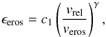${\mathit{ϵ}}_{\mathrm{eros}}\mathrm{=}{\mathit{c}}_{\mathrm{1}}{\left(\frac{{\mathit{v}}_{\mathrm{rel}}}{{\mathit{v}}_{\mathrm{eros}}}\right)}^{\mathit{\gamma }}\mathit{,}$(13)with c₁ ~ 1 (Güttler et al. 2010; Seizinger et al. 2013). While in supersonic cratering collisions γ = 16/9 (Tielens et al. 1994), the velocities encountered in this work are not that high and at most comparable to the sound speed in porous aggregates (Paszun & Dominik 2008). Hence, we will use γ = 1, in agreement with both numerical and experimental work in the appropriate velocity range (Güttler et al. 2010; Schräpler & Blum 2011; Seizinger et al. 2013).

Lastly, we need a prescription for the filling factors after an erosive collision. We assume that i) the filling factor of the target remains unchanged; and ii) the filling factor of the fragments is found by assuming they have the same fractal dimension as the target, where the target’s fractal dimension D_f is estimated as ${\mathit{D}}_{\mathrm{f}}\mathrm{\simeq }\mathrm{3}{\left[\mathrm{1}\mathrm{-}\frac{\log \mathrm{\left(}\mathit{\phi }\mathrm{\right)}}{\log \mathrm{(}\mathit{m}\mathit{/}{\mathit{m}}_{\mathrm{0}}\mathrm{)}}\right]}^{-1}\mathrm{·}$(14)The assumptions of the erosion model employed in this work are discussed further in Sect. 6.

2.4. Aggregate compaction

An aggregate’s porosity can be altered through collisions, or through non-collisional mechanisms. In this section, we first describe how porosity can increase and decrease as the result of sticking collisions. Then, we discuss gas- and self-gravity compaction.

2.4.1. Collisional compaction

When two particles i and j collide at a relative velocity v_rel that is below the thresholds for fragmentation or erosion, the particles stick, and form a new aggregate with mass m_i + m_j. The internal density of the new particle depends on how the impact energy compares to the energy needed for restructuring. When the impact energy is not enough to cause significant restructuring, particles grow by hit-and-stick collisions, and very fractal aggregates can be formed (Kempf et al. 1999). When the impact energy is much larger, significant restructuring can take place, reducing the internal density of the dust aggregates. In this work, we will make use of the model presented in Suyama et al. (2012) and Okuzumi et al. (2012). Specifically, we use Eq. (15) of Okuzumi et al. (2012) to calculate the volume of the a newly-formed aggregate, as a function of the masses and volumes of particles i and j, the impact velocity, and the rolling energy E_roll; the energy needed to roll two monomers over an angle of 90° (Dominik & Tielens 1997).

Gundlach et al. (2011) measured the rolling force between ice particles with radii of ~1.5 μm to be 1.8 × 10^-3 dyn, implying a rolling energy of 1.8 × 10^-7 erg. Assuming the rolling force is size-independent (Dominik & Tielens 1995), the rolling energy is then often extrapolated using E_roll ∝ a₀. Recently however, Krijt et al. (2014) showed that the rolling force scales with the size of the area of the monomers that is in direct contact, resulting in ${\mathit{F}}_{\mathrm{roll}}\mathrm{\propto }{\mathit{a}}_{\mathrm{0}}^{\mathrm{2}\mathit{/}\mathrm{3}}$, and ${\mathit{E}}_{\mathrm{roll}}\mathrm{\propto }{\mathit{a}}_{\mathrm{0}}^{\mathrm{5}\mathit{/}\mathrm{3}}$, leading to significantly smaller rolling energies when extrapolating down to monomer radii well below a micrometer. In this work, we use the scaling law of Krijt et al., resulting in a rolling energy of 4 × 10^-9 erg for 0.1-μm radius ice particles. Physically, a lower rolling energy means less energy is needed to start restructuring of an aggregate. As a result, a lower rolling energy will lead to compacter aggregates.

2.4.2. Gas and self-gravity compaction

Aggregates can also be compressed by the ram pressure of the gas, or their own gravity, if they become very porous or massive. For low internal densities, Kataoka et al. (2013b) found that the external pressure a dust aggregate can just withstand equals 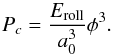${\mathit{P}}_{\mathit{c}}\mathrm{=}\frac{{\mathit{E}}_{\mathrm{roll}}}{{\mathit{a}}_{\mathrm{0}}^{\mathrm{3}}}{\mathit{\phi }}^{\mathrm{3}}\mathit{.}$(15)This pressure can then be compared to the pressure arising form the surrounding gas and from self-gravity 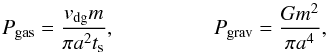${\mathit{P}}_{\mathrm{gas}}\mathrm{=}\frac{{\mathit{v}}_{\mathrm{dg}}\mathit{m}}{\mathit{\pi }{\mathit{a}}^{\mathrm{2}}{\mathit{t}}_{\mathrm{s}}}\mathit{,}{\mathit{P}}_{\mathrm{grav}}\mathrm{=}\frac{\mathit{G}{\mathit{m}}^{\mathrm{2}}}{\mathit{\pi }{\mathit{a}}^{\mathrm{4}}}\mathit{,}$(16)with G the gravitational constant, in order to see whether an aggregate will be compacted as a result of these non-collisional processes (Kataoka et al. 2013a). In this work, we will take these effects into account in a self-consistent way, while calculating the collisional evolution of the dust distribution.

3. Monte Carlo approach

Numerical techniques for studying coagulation can be divided in two categories²: integro-differential methods (e.g., Weidenschilling 1980; Dullemond & Dominik 2005; Birnstiel et al. 2010), and Monte Carlo (MC) methods (Gillespie 1975; Ormel et al. 2007; Zsom & Dullemond 2008). Tracing particle porosity as well as mass becomes computationally expensive in the integro-differential approach. A solution to this issue was presented by Okuzumi et al. (2012), who assumed the porosity distribution for a given mass bin was narrow, but could vary in time. Since we are interested in including erosive processes, this assumption is not expected to hold, and for this reason we opt for the MC method.

The approach to calculate the collisional evolution is based on the distribution method as described in Ormel & Spaans (2008). In this section we briefly revisit the method, focussing on what is new in this work.

We let f(x) be the (time-dependent) particle distribution function, with x_i the unique parameters describing dust particle i, in our case mass and filling factor³. For every pair of particles i and j, one can determine the collision rate as ${\mathit{C}}_{\mathit{ij}}\mathrm{=}{\mathit{K}}_{\mathit{ij}}\mathit{/}\mathrm{𝒮}\mathit{,}$(17)with the surface area of the column⁴, and K_ij the collision kernel, which in this case equals 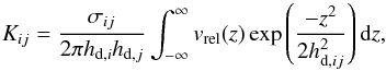${\mathit{K}}_{\mathit{ij}}\mathrm{=}\frac{{\mathit{\sigma }}_{\mathit{ij}}}{\mathrm{2}\mathit{\pi }{\mathit{h}}_{\mathrm{d}\mathit{,i}}{\mathit{h}}_{\mathrm{d}\mathit{,j}}}{\mathrm{\int }}_{\mathrm{-}\mathrm{\infty }}^{\mathrm{\infty }}{\mathit{v}}_{\mathrm{rel}}\mathrm{\left(}\mathit{z}\mathrm{\right)}\exp \left(\frac{\mathrm{-}{\mathit{z}}^{\mathrm{2}}}{\mathrm{2}{\mathit{h}}_{\mathrm{d}\mathit{,ij}}^{\mathrm{2}}}\right)\mathrm{d}\mathit{z,}$(18)where h_d,i is given by Eq. (6), and 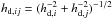${\mathit{h}}_{\mathrm{d}\mathit{,ij}}\mathrm{=}\mathrm{(}{\mathit{h}}_{\mathrm{d}\mathit{,i}}^{-2}\mathrm{+}{\mathit{h}}_{\mathrm{d}\mathit{,j}}^{-2}{\mathrm{)}}^{\mathrm{-}\mathrm{1}\mathit{/}\mathrm{2}}$ and σ_ij = π(a_i + a_j)² equals the collisional cross section (Okuzumi et al. 2012). This rate equation takes into account that particles with different properties inhabit different vertical scale heights, and is correct as long as the coagulation timescale is longer than the vertical settling/diffusion timescale. In this work, we approximate the integral over z by assuming the midplane relative velocity is a good indication for v_rel throughout the column. This allows us to solve the integral analytically and write 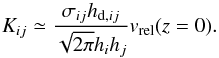${\mathit{K}}_{\mathit{ij}}\mathrm{\simeq }\frac{{\mathit{\sigma }}_{\mathit{ij}}{\mathit{h}}_{\mathrm{d}\mathit{,ij}}}{\sqrt{\mathrm{2}\mathit{\pi }}{\mathit{h}}_{\mathit{i}}{\mathit{h}}_{\mathit{j}}}{\mathit{v}}_{\mathrm{rel}}\mathrm{(}\mathit{z}\mathrm{=}\mathrm{0}\mathrm{)}\mathit{.}$(19)For the purpose of this paper, this approximation is sufficiently accurate, since most of the growth is expected to take place near the midplane.

Then, we can define the total collision rate for particle C_i = ∑ _j>iC_ij, and the total collision rate C_tot = ∑ _iC_i. With all these rates known, 3 random numbers are used to identify which particles collide, and the time Δt after which this collision occurs. The colliding particles are then removed from f, and the collision product is added. As a result, all collision rates C_i have to be adjusted, since the particle distribution f has changed. This cycle is then repeated.

The simple method has two main drawbacks. First, the time needed for updating the rates in between collisions scales with N², where N is the total number of particles. Second, this method describes 1 collision per cycle, which can become a problem whenever the mass distribution is broad.

3.1. Grouping method

Rather than following every particle individually, identical particles can be grouped together. In our approach, the dust distribution is described by N_f particle families. Within a single family, all particles have identical properties, in our case mass and internal density. In every family i, there are w_i particle groups, each containing 2^z_i individual particles, where we call z_i the zoom factor. The total number of particles in a single family therefor equals g_i = w_i2^z_i, and the total number of particles is N = ∑ _ig_i. Instead of 2 particles colliding per cycle, collisions now happen between groups of particles (see Ormel & Spaans 2008, for details about this method). Letting i refer to the group with the lower zoom factor, we obtain for the group collision rates 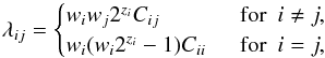${\mathit{\lambda }}_{\mathit{ij}}\mathrm{=}\{\begin{array}{c}\\ & \mathrm{for}\mathit{i}\ne \mathit{j,}\\ & \mathrm{for}\mathit{i}\mathrm{=}\mathit{j,}\end{array}$(20)where the i = j case in Eq. (20) describe so-called in-group collisions. Like before, we can define the total collision rate per family λ_i = ∑ _{j ≥ i}λ_ij, and the total collision rate λ_tot = ∑ _iλ_i, which can be used to determine which groups collide and when. This grouped approach has tremendous advantages, but there are also pitfalls, which we discuss in the following section.

3.2. Sequential collisions

Imagine the collision between a group of large bodies i with a group of much smaller bodies j, such that m_i ≫ m_j. Thus, a total of 2^z_ii-particles will collide with 2^z_jj-particles. Assuming z_j ≫ z_i, every i-particle in the group will collide with 2^{z_j − z_i}j-particles in a single sequence before the collision rates are updated and the next groups to collide are chosen. We are assuming that the collision rates and the relative velocity between i and j particles are constant during this sequence, but this is only true if the properties of particle i do not change significantly. For this reason we include the group splitting factor N_ε, that limits the number of collisions to 2^{z_j − z_i − N_ε}.

We let δm_i be the change in the mass of the larger particle i, after a single collision with a j-particle. Assuming the changes are small, we can then extrapolate to find the total change after the full sequence of collisions 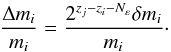$\frac{\mathrm{\Delta }{\mathit{m}}_{\mathit{i}}}{{\mathit{m}}_{\mathit{i}}}\mathrm{=}\frac{{\mathrm{2}}^{{\mathit{z}}_{\mathit{j}}\mathrm{-}{\mathit{z}}_{\mathit{i}}\mathrm{-}{\mathit{N}}_{\mathit{\epsilon }}}\mathit{\delta }{\mathit{m}}_{\mathit{i}}}{{\mathit{m}}_{\mathit{i}}}\mathrm{·}$(21)Now, by imposing that (Δm_i/m_i) ≤ f_m, we obtain ${\mathit{N}}_{\mathit{\epsilon }}^{\mathrm{\left(}\mathit{m}\mathrm{\right)}}\mathrm{=}\left[\mathrm{-}{\log }_{\mathrm{2}}\left(\frac{{\mathit{f}}_{\mathit{m}}{\mathit{m}}_{\mathit{i}}{\mathrm{2}}^{{\mathit{z}}_{\mathit{i}}}}{\mathit{\delta }{\mathit{m}}_{\mathit{i}}{\mathrm{2}}^{{\mathit{z}}_{\mathit{j}}}}\right)\right]\mathit{,}$(22)where the square brackets indicate that ${\mathit{N}}_{\mathit{\epsilon }}^{\mathrm{\left(}\mathit{m}\mathrm{\right)}}$ is truncated to integers ≥ 0, which has the effect of particles with mass ratios ≥ f_m always colliding 1-on-1. In the case of perfect sticking, obviously δm_i = m_j, and Eq. (22) reduces to Eq. (12) of Ormel & Spaans (2008). We write an equivalent expression for the filling factor of the bigger grain ${\mathit{N}}_{\mathit{\epsilon }}^{\mathrm{\left(}\mathit{\phi }\mathrm{\right)}}\mathrm{=}\left[\mathrm{-}{\log }_{\mathrm{2}}\left(\frac{{\mathit{f}}_{\mathit{\phi }}{\mathit{\phi }}_{\mathit{i}}{\mathrm{2}}^{{\mathit{z}}_{\mathit{i}}}}{\mathit{\delta }{\mathit{\phi }}_{\mathit{i}}{\mathrm{2}}^{{\mathit{z}}_{\mathit{j}}}}\right)\right]\mathit{,}$(23)where δφ_i denotes the change in φ after a single collision. 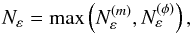The two limits are combined by writing ${\mathit{N}}_{\mathit{\epsilon }}\mathrm{=}\begin{array}{c}\max \end{array}\mathrm{(}{\mathit{N}}_{\mathit{\epsilon }}^{\mathrm{\left(}\mathit{m}\mathrm{\right)}}\mathit{,}{{\mathit{N}}_{\mathit{\epsilon }}^{\mathrm{\left(}\mathit{\phi }\mathrm{\right)}}}^{\mathrm{)}}\mathit{,}$(24)and ensure that neither the filling factor, nor the mass of the larger particle change by too much during a single MC cycle. We note that N_ε is not only a function of the masses and densities of both particles, but also of the relative velocity, since this influences δφ_i (and δm_i, when erosion is present). In this work, we will typically use f_m = f_φ = 0.1.

Imposing this limit has two consequences. First, since the group of i-particles can now only collide with part of the group of j-particles, this needs to be taken into account when the group collision rates are calculated, changing Eq. (20) into 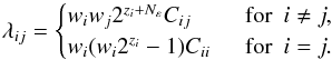${\mathit{\lambda }}_{\mathit{ij}}\mathrm{=}\{\begin{array}{c}\\ & \mathrm{for}\mathit{i}\ne \mathit{j,}\\ & \mathrm{for}\mathit{i}\mathrm{=}\mathit{j}\mathit{.}\end{array}$(25)Second, since it can occur that only part of a group collides, group numbers w_i can now become fractional. This is fine as long as w_i ≥ 1, ensuring that at least one full group collision can occur in the future (Ormel & Spaans 2008).

3.3. The distribution method

For a given number of family members g_i, we have some freedom in choosing z_i; either creating many groups with a few members (low z_i) or a few groups with many members (high z_i). This choice for the zoom factors is crucial because it determines how many groups of a certain mass exist, which is related to the numerical resolution in that part of the mass range. Two approaches for determining the zoom factors have been proposed by Ormel & Spaans (2008).

One approach is the so-called equal mass method, in which one strives to have groups of equal total mass. This method is essentially identical to the method of Zsom & Dullemond (2008). With this approach, the peak of the mass distribution is very well traced, but parts of the particle distribution that carry little mass are described by a few groups, resulting in larger uncertainties. The second option is the distribution method, where one strives to have an equal number of groups per mass decade, independent of the total mass present in that interval. The difference between the two methods is nicely illustrated in Fig. 4 of Ormel & Spaans (2008). Since we are interested in erosion, it is crucial to resolve the particle distribution over the entire mass range. It is for that reason that we adopt the distribution method.

In practice, this means that at certain times during the simulation, we calculate the total number of particles N₁₀ in every mass decade. The optimal zoom number for families in that mass range then equals ${\mathit{z}}^{\mathrm{\ast }}\mathrm{=}\left[{\log }_{\mathrm{2}}\left(\frac{{\mathit{N}}_{\mathrm{10}}}{{\mathit{w}}^{\mathrm{\ast }}}\right)\right]\mathit{,}$(26)where w^∗ is the desired number of groups per mass decade. In this way, we construct a function z^∗(m), which gives the desired zoom number for a family with particle mass m. We then check every existing family: if a certain zoom number is too big, we magnify the group (z_i → z_i − 1, w_i → 2w_i) until z_i = z^∗(m_i). Similarly, if the zoom number is too small, we demagnify (z_i → z_i + 1, w_i → w_i/ 2). The (de)magnification process conserves particle number, but does force one to update the various collision rates. A more detailed description of (de)magnification is given by Ormel & Spaans (2008). In the rest of this work, we calculate and update the zoom factors after every 10² collision cycles, whenever the peak or average mass has changed by > 5%, or when the maximum mass has changed by > 50%, which we found to ensure a smooth evolution of the zoom factors. We will use w^∗ = 60 for the perfect sticking calculations, and w^∗ = 40 for the ones including erosion.

3.4. Merging

Lastly, we have to address the merging of families. It can occur that demagnification results in a group number w_i< 1, which is not allowed. When this occurs, the family does not contain enough individual particles to adopt z_i = z^∗(m_i). At this point, the family is insignificant. As we are simulating a fixed volume and the total mass needs to be conserved, we merge the family with another, healthy (meaning w_i> 1) one. First, we find the family j that resembles family i the most. In order to do so, we find the family that gives the largest product (R^(m))(R^(φ))³, where R^(φ) ≤ 1 is the ratio of the filling factors⁵. Then, we merge the families into a new family k with properties 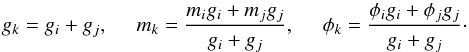${\mathit{g}}_{\mathit{k}}\mathrm{=}{\mathit{g}}_{\mathit{i}}\mathrm{+}{\mathit{g}}_{\mathit{j}}\mathit{,}{\mathit{m}}_{\mathit{k}}\mathrm{=}\frac{{\mathit{m}}_{\mathit{i}}{\mathit{g}}_{\mathit{i}}\mathrm{+}{\mathit{m}}_{\mathit{j}}{\mathit{g}}_{\mathit{j}}}{{\mathit{g}}_{\mathit{i}}\mathrm{+}{\mathit{g}}_{\mathit{j}}}\mathit{,}{\mathit{\phi }}_{\mathit{k}}\mathrm{=}\frac{{\mathit{\phi }}_{\mathit{i}}{\mathit{g}}_{\mathit{i}}\mathrm{+}{\mathit{\phi }}_{\mathit{j}}{\mathit{g}}_{\mathit{j}}}{{\mathit{g}}_{\mathit{i}}\mathrm{+}{\mathit{g}}_{\mathit{j}}}\mathrm{·}$(27)The new zoom- and group numbers are chosen such that z_k = z^∗(m_k). Merging is necessary to suppress the total number of groups.

3.5. Non-collisional compaction

Non-collisional compaction is implemented as follows: whenever a new aggregate is created in a collision, we calculate its compressive strength using Eq. (15), and compare this to the external pressures from gas ram pressure and self-gravity, calculated with Eq. (16) (Kataoka et al. 2013a). If either one of the external pressures exceeds P_c, we compactify the dust grain (i.e., increase φ) until the aggregate can withstand the external pressures.

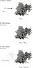Fig. 3 a) Schematic of a collision between unequal particles with a mass ratio R(m) = (mproj/mtarget) ≪ 1. b) Sticking occurs when vrel<veros. The mass of the projectile is added to the target. c) Collisions above the erosion threshold velocity lead to erosion. The mass loss of the target is given by the erosion efficiency ϵeros and the mass of the projectile.

3.6. Erosion

For every collision, we check if the conditions for erosion are met (i.e., v_rel>v_eros and ${\mathit{R}}^{\mathrm{\left(}\mathit{m}\mathrm{\right)}}\mathit{<}{\mathit{R}}_{\mathrm{crit}}^{\mathrm{\left(}\mathit{m}\mathrm{\right)}}$), and if so, we determine the erosion efficiency using Eq. (13). After a single erosive event, the mass that does not end up in the target body equals (1 + ϵ_eros)m_proj, see Fig. 3. To limit the number of new families, we redistribute this mass over fragments with a mass of m_frag = m_proj/ 10.

4. Results

In this section we show the results of our simulations for different erosion recipes, compaction mechanisms, turbulence strengths, and disk locations. When discussing the particle distribution at a given time, we shall use a number of quantities. These are the average mass and porosity ${\mathit{m}}_{\mathit{a}}\mathrm{=}\mathrm{⟨}{\mathit{m}}_{\mathit{i}}\mathrm{⟩}\mathit{,}{\mathit{\phi }}_{\mathit{a}}\mathrm{=}\mathrm{⟨}{\mathit{\phi }}_{\mathit{i}}\mathrm{⟩}\mathit{,}$(28)which trace the properties of the average particle, and the peak mass and filling factor ${\mathit{m}}_{\mathrm{p}}\mathrm{=}\frac{\mathrm{⟨}{\mathit{m}}_{\mathit{i}}^{\mathrm{2}}\mathrm{⟩}}{\mathrm{⟨}{\mathit{m}}_{\mathit{i}}\mathrm{⟩}}\mathit{,}{\mathit{\phi }}_{\mathit{p}}\mathrm{=}\frac{\mathrm{⟨}{\mathit{m}}_{\mathit{i}}{\mathit{\phi }}_{\mathit{i}}\mathrm{⟩}}{\mathrm{⟨}{\mathit{m}}_{\mathit{i}}\mathrm{⟩}}\mathit{,}$(29)which trace the properties of the mass-dominating particle. We will also use the maximum mass m_max, which is simply the mass of most massive particle.

4.1. Perfect sticking

4.1.1. Collisional-compaction-only scenario

As a test for the MC approach, we attempt first to match the trends observed in Okuzumi et al. (2012), who assumed perfect sticking between the dust grains. We adopt a turbulence strength parameter of α = 10^-3, and focus on a vertical column at 5 AU in a typical MMSN disk. At this point, we only include collisional compaction and omit erosion. To allow a direct comparison to the work of Okuzumi et al., we do not include the effects of Newton drag for particles with large Reynolds numbers in this simulation. In the rest of this work, Newton drag is always included self-consistently.

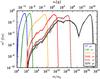Fig. 4 Evolution of the normalized particle mass distribution at 5 AU with α = 10-3, assuming perfect sticking and without compaction through gas and self-gravity. Only Epstein are Stokes drag are considered. Solid lines indicate averages over 4 MC runs with identical starting conditions, and the shaded areas represent a spread of 1σ.

Figure 4 shows the evolution of the normalized mass distribution m²f(m) as a function of time. Solid lines mark the average over 4 MC runs. Thanks to the distribution method described in Sect. 3.3, the sampling of the mass distribution is very good over the entire mass range: even at later times, when most of the mass is located in particles with masses of ~10¹⁵ g, the distribution of particles all the way down to 10^-9 g is resolved remarkably well, despite these particles only making up a very small fraction of the total mass.

When we compare our Fig. 4 to Fig. 7 of Okuzumi et al. (2012), it is clear that our local MC method yields very similar results. We recognize the familiar narrow mass peak when growth is governed by Brownian motion, followed by a broader distribution once turbulence kicks in. Once particles reach Ωt_s ~ 1 (m_j ≃ 10¹⁰ g in this case), systematic drift greatly increases their collision rate, and very rapid growth ensues. The slight difference in timescales is attributed to i) the slightly different value for the rolling energy, ii) our approximation of Eq. (18), and iii) our use Eq. (8) to calculate the stopping times, while Okuzumi et al. used ${\mathit{t}}_{\mathrm{s}}\mathrm{=}{\mathit{t}}_{\mathrm{s}}^{\mathrm{\left(}\mathrm{Ep}\mathrm{\right)}}\mathrm{+}{\mathit{t}}_{\mathrm{s}}^{\mathrm{\left(}\mathrm{St}\mathrm{\right)}}$ to ensure a smooth transition between Epstein and Stokes drag (Okuzumi, priv. comm.).

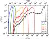Fig. 5 Like Fig. 4, but with compaction through gas and self-gravity and Newton drag for particles with Rep> 1.

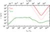Fig. 6 Evolution of the growth- and radial drift timescale of the peak mass for the perfect sticking model at 5 AU with α = 10-3. The dotted line indicates (tdrift/ 30). Only collisional compaction has been taken into account.

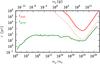Fig. 7 Evolution of the growth- and radial drift timescale of the peak mass for the perfect sticking model at 5 AU with α = 10-3. The dotted line indicates (tdrift/ 30). Compaction from gas and self-gravity, and Newton drag have been taken into account.

While we take into account drift-induced relative velocities, the dust particles are bound to our simulated column and cannot move radially through the disk. To test the validity of this assumption, we compare the growth timescale of the peak mass, defined as 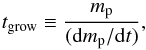${\mathit{t}}_{\mathrm{grow}}\mathrm{\equiv }\frac{{\mathit{m}}_{\mathrm{p}}}{\mathrm{(}\mathrm{d}{\mathit{m}}_{\mathrm{p}}\mathit{/}\mathrm{d}\mathit{t}\mathrm{)}}\mathit{,}$(30)to the radial drift timescale at that mass 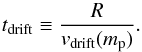${\mathit{t}}_{\mathrm{drift}}\mathrm{\equiv }\frac{\mathit{R}}{{\mathit{v}}_{\mathrm{drift}}\mathrm{\left(}{\mathit{m}}_{\mathrm{p}}\mathrm{\right)}}\mathit{.}$(31)The radial drift velocity is given by (Weidenschilling 1977) ${\mathit{v}}_{\mathrm{drift}}\mathrm{=}\mathrm{-}\frac{\mathrm{2}\mathrm{\Omega }{\mathit{t}}_{\mathrm{s}}}{\mathrm{1}\mathrm{+}\mathrm{(}\mathrm{\Omega }{\mathit{t}}_{\mathrm{s}}{\mathrm{)}}^{\mathrm{2}}}\mathit{\eta }{\mathit{v}}_{\mathrm{K}}\mathit{,}$(32)where v_K = RΩ is the Keplerian orbital velocity, and η can be written as (Nakagawa et al. 1986) 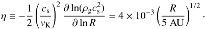$\mathit{\eta }\mathrm{\equiv }\mathrm{-}\frac{\mathrm{1}}{\mathrm{2}}{\left(\frac{{\mathit{c}}_{\mathrm{s}}}{{\mathit{v}}_{\mathrm{K}}}\right)}^{\mathrm{2}}\frac{\mathit{\partial }\ln \mathrm{\left(}{\mathit{\rho }}_{\mathrm{g}}{\mathit{c}}_{\mathrm{s}}^{\mathrm{2}}\mathrm{\right)}}{\mathit{\partial }\ln \mathit{R}}\mathrm{=}\mathrm{4}\mathrm{\times }{\mathrm{10}}^{-3}{\left(\frac{\mathit{R}}{\mathrm{5}\mathrm{AU}}\right)}^{\mathrm{1}\mathit{/}\mathrm{2}}\mathrm{·}$(33)Figure 6 shows both the growth and radial drift timescales during the complete evolution of the peak mass. Initially, relative velocities are dominated by Brownian motion. Since this velocity drops with increasing particle mass, the growth timescale increases. Around a mass of 10^-9 g, turbulent velocities start to dominate the relative velocity, and the growth timescale stays approximately constant. Particles larger than 10³ g enter the second turbulent regime as t_s(m_p) >t_η. In this regime, velocities between similar particles are increased (see Eq. (11)), which leads to a decrease in the growth timescale. Since the growth timescale is always much smaller than the drift timescale, the aggregates in this simulation do indeed out-grow the radial drift barrier.

4.1.2. Including gas and self-gravity compaction

The next step is to include compaction by gas pressure and self-gravity, as described in Sect. 2.4.2. In addition, we now take into account Newton drag for particles with large Reynolds numbers. Figure 5 shows the results for the same disk parameters as before. The general shape of the evolution looks similar to Fig. 4 initially, but from the corresponding times it is clear that the growth is slower for the largest aggregates. The main reason for this is that the largest dust grains are compacted by the gas and self-gravity, resulting in a smaller collisional cross section. In addition, the aerodynamic properties are different, which affects the relative velocities.

The growth- and drift timescales are plotted in Fig. 7. When we compare Figs. 6 and 7, we confirm that the growth close to the drift barrier is slower when using the full compaction recipe. For the largest particles, the growth timescale is increased by more than 2 orders of magnitude. In addition, including Newton drag has broadened the drift barrier somewhat. Nonetheless, the growth is still fast enough to prevent particles from drifting significant distances.

4.1.3. Evolution of internal densities

It is interesting to compare the evolution of the internal densities of the particles for the models with and without non-collisional compaction. In Fig. 8, the peak filling factor is plotted versus the peak mass for the simulations described so far. The symbols correspond to important points in the evolution of the aggregates: open circles are related to the stopping time of the aggregates, and closed symbols indicate the onset of various compaction mechanisms⁶.

Initially, aggregates grow through hit-and-stick collisions, and evolve along a line of constant fractal dimension close to 2. In the collisional-compaction-only scenario, particles reach a filling factor of ~10^-5 during hit and stick growth, before collisional compaction kicks in, after which φ stays almost constant. When Ωt_s(m_p) > 1, the internal density drops even further. The general picture, as well as the location of the various turnover points, is consistent with the top panel of Fig. 10 of Okuzumi et al. (2012). When non-collisional compaction is included, the filling factor, in general, is much higher at later times, and follows the boundaries that have been described by Kataoka et al. (2013a; e.g., their Fig. 3). For this particular combination of turbulence, rolling energy, and monomer size, compacting by gas ram pressure actually occurs before the first collisional compaction event takes place⁷. Significant settling occurs when Ωt_s>α, which corresponds to m ~ 10^-3 g for compact particles (see Fig. 1). From Fig. 8 however, we see that porous particles only begin to settle when their masses reach ~10⁴−10⁵ g. Lastly, aggregates with masses above ~10¹⁰ g are compacted by self-gravity, causing the filling factor for the largest bodies to be several orders of magnitude higher. In the remainder of this work, we include both collisional and non-collisional compaction mechanisms, and Epstein, Stokes, and Newton drag self-consistently.

Fig. 8 Evolution of the internal structure of the mass-dominating particles, for the perfect sticking models at 5 AU, for the models with and without non-collisional compaction mechanisms. Aggregates start out as monomers in the top left corner, and grow towards larger sizes and porosities. Lines show individual simulations. Open symbols correspond to points where the mass dominating particles reach a = λmfp (°); ts = tη (◇); Ωts = α (▿); and Ωts = 1 (□). Filled symbols show peak mass and filling factor at the times of first: collisional compaction (⋆); gas-pressure compaction (◆); and self-gravity compaction (•).

4.2. Erosion

With this framework in place, the final step is to include the erosion model of Sect. 2.3.3 in the simulations, and calculate the evolution of the particle distribution self-consistently. Figure 9 shows the mass distribution at various times for v_eros = 20 m s^-1. Initially, the evolution proceeds just like in 5, but as the largest aggregates approach Ωt_s = 1, their velocity relative to smaller particles is high enough for erosion, and their growth stalls. As a direct consequence of the erosion, the amount of small particles increases, and after ~4000 yr a steady-state is reached, with a significant amount of mass residing in particles smaller than a few grams.

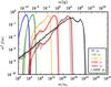Fig. 9 Evolution of the normalized particle mass distribution at 5 AU with α = 10-3, assuming veros = 20 m s-1. The full compaction model is used.

To investigate how erosion halts the growth of the largest bodies, it is instructive to plot so-called projectile mass distributions (Okuzumi et al. 2009). For a certain particle mass m_t, these distributions show the contribution to the growth of that particle as a function of projectile mass m ≤ m_t. An example of such a plot is shown in Fig. 9 of Okuzumi et al. (2012), where the distribution function is plotted at various times for m_t = m_p. For our distribution plots, we make two important changes: first, since we are interested in the growth of the largest bodies, we plot projectile distributions for m_t = m_max, with m_max the largest mass in the simulation at a given time. Second, to illustrate the effect of erosive collisions, we calculate the mass loss for every erosive collision, taking into account the correct erosion efficiency⁸. As a result, the sign of the distribution function can be both positive and negative. Figure 10 shows the distribution for one of the simulations of Fig. 9 (colors correspond to the same times). When we examine the right-most projectile mass distribution, corresponding to a time t = 10⁴ yr, it is immediately clear how erosion affects the evolution of particles with Ωt_s ~ 1. While these aggregates grow by collisions with similar-sized bodies, they lose mass by colliding with particles that have a mass below 10^-2m_t. This could have been predicted by looking at Fig. 2, from which it is clear that the highest velocities are attained between particles with mass ratios well below unity. The importance of this erosion however, depends on the current mass distribution, and can only be tested through dedicated simulations like the ones presented here. Since the area under the negative part of the projectile distribution outweighs the positive part, the erosion is so effective that it stops the growth of the largest bodies, resulting in the behavior seen in Fig. 9.

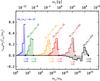Fig. 10 Projectile distribution mass functions for simulation E1, constructed for the maximum masses (mt =•) at various times. Colors and times correspond to Fig. 9. For each distribution, the stopping time of the mt-particle is given, and the weights of the total positive and negative area are plotted. The distributions have been normalized in such a way, that the absolute sum of the contributions equals 1.

We define a parameter ζ using the positive and negative areas under the projectile mass distributions 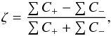$\mathit{\zeta }\mathrm{=}\frac{\sum {\mathit{C}}_{\mathrm{+}}\mathrm{-}\sum {\mathit{C}}_{\mathrm{-}}}{\sum {\mathit{C}}_{\mathrm{+}}\mathrm{+}\sum {\mathit{C}}_{\mathrm{-}}}\mathit{,}$(34)with ∑ C₊ and ∑ C₋ the sums of the positive and negative part of the projectile mass distribution respectively. The parameter ζ ranges from 1 (no erosion) to –1 (only erosion), and equals 0 when there is a balance between growth and erosion.

The top panel of Fig. 11 shows the evolution of ζ for the most massive particle during one of the simulations of Fig. 9, plotted as a function of Ωt_s of the maximum mass. Early on, there is no erosion present and ζ = 1, but as the largest bodies grow towards Ωt_s = 1, erosion increases and ζ drops. When 0 <ζ< 1, the massive particles still grow faster then they are eroded, but the erosion can be significant in that it results in the creation of more small particles, thus increasing its destructive effect. When ζ< 0, erosion dominates over growth and the most massive particles are loosing considerable mass. This causes the curve in Fig. 11 to turn around. As bodies shrink, there is less erosion and ζ increases again. A quasi steady-state is reached with ζ just below unity and Ωt_s(m_max) ~ 0.6. The reason ζ ≠ 0 during the steady state, is that it is not the same particle that is the most massive at all times. Instead, particles take turn at being the most massive body. Since the largest particles are stuck at a mass and size for which drift is fastest, they will move radially towards the central star. For this combination of parameters, we conclude that growth beyond the drift barrier is impeded by erosion.

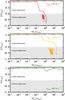Fig. 11 Evolution of ζ(mmax) for erosive simulations with veros = 20,40,60 m s-1 as a function of Ωts(mmax), showing the impact of erosion on the ability of the largest bodies to grow. In the upper two panels, the steady-state is indicated by the ⊚-symbol.

The other panels of Fig. 11 show similar plots but for different erosion threshold velocities. For v_eros = 40 m s^-1 (middle panel), erosion is less efficient and the largest bodies grow to Ωt_s ≃ 10 before they start to lose mass rapidly. The reason particles can grow larger is twofold. First, the threshold velocity itself is somewhat higher, causing erosion to start for higher masses. Second, since the erosion efficiency is proportional to (v_rel/v_eros), the high-velocity projectile are less efficient in excavating mass from the targets. Both effects together cause the largest mass in the steady state to be about a factor of 10 larger than in the top panel of Fig. 11. Finally, the bottom panel shows the results for v_eros = 60 m s^-1. This is a special case, since now the erosion threshold velocity can only be reached around Ωt_s = 1, with radial drift, azimuthal drift, and turbulence contributing (see Fig. 2). Indeed, erosion is strongest around Ωt_s = 1, but it is inefficient and ζ never drops below 0. When Ωt_s> 20, erosion reappears, as a result of smaller particles drifting into the larger bodies, but since ζ ~ 1, bodies can continue to grow relatively unaffected.

Fig. 12 Masses and filling factors of all unique families at different times, for simulation E1. One dot corresponds to one family, and does not provide information about the total mass or number of members in that family.

4.2.1. Variation in porosity

One of the biggest advantages of the MC method is that aggregate mass and porosity are treated truly independently. In other words, aggregates of identical mass can have a very different porosity. However, the collision model used in this work immediately implies that the spread in porosities (for a given particle mass) will be narrow, when sticking collisions dominate the evolution. For example, the collision model, at the moment, does not include an impact-parameter dependence in collisions, or a random component in the relative velocity. As a result, collisions between particles with certain properties always occur at the same relative velocity, and always result in the same collision product(s). Moreover, when gas compaction (or self-gravity compaction) limits the porosity of an aggregate, bodies will evolve along P_c = P_gas (or P_c = P_grav), according to Eqs. (15) and (16). As a result, mass-porosity relations as shown in Fig. 8 accurately represent the internal structure of the majority of aggregates.

This picture changes when erosion starts to play a role. Figure 12 shows the evolution of the properties of each family in one of the E1 simulations. We note that each dot corresponds to a single family, and that the total masses and number of family members can vary significantly between families. Nonetheless, Fig. 12 gives a good indication of the spread in porosity. For the reasons described above, the spread in porosity is very small during the first 3000 years of the evolution. After 3400 years, the first erosive collisions have occurred, and created a population of fragments with a fractal dimension set by the parent body. At this point, the porosity distribution becomes bimodal, and the assumption of a single porosity parameter – which only depends on aggregate mass – is untenable. Later, after ~6000 years, the original population of aggregates, whose porosity was set by their growth history, has disappeared. A steady-state is reached in which the internal structure of the fragments is dominated by the porosity of the particles that act as targets for erosion, i.e., the large bodies with Ωt_s ~ 1.

5. Semi-analytical model

The evolution of the mass-dominating particles can be captured in a simple semi-analytical model. Assuming the entire dust mass is located in particles of identical mass m_p, the growth rate can be written as (Okuzumi et al. 2012) 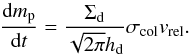$\frac{\mathrm{d}{\mathit{m}}_{\mathrm{p}}}{\mathrm{d}\mathit{t}}\mathrm{=}\frac{{\mathrm{\Sigma }}_{\mathrm{d}}}{\sqrt{\mathrm{2}\mathit{\pi }}{\mathit{h}}_{\mathrm{d}}}{\mathit{\sigma }}_{\mathrm{col}}{\mathit{v}}_{\mathrm{rel}}\mathit{.}$(35)The collisional cross section depends directly on the particle porosity, and the relative velocity and dust scale height depend on φ through the particle stopping time. As a simple model for the aggregate’s internal structure, we assume the aggregates initially grow with a constant fractal dimension of ~2, until the kinetic energy in same-sized collisions exceeds E_roll. After that, the internal structure can be calculated through Eq. (31) of Okuzumi et al. (2012), but in practice is always dominated by the gas/self-gravity compression of Kataoka et al. (2013a), see Sect. 2.4.2.

This approach, similar to Kataoka et al. (2014, Sect. 5.3), is valid when particles grow primarily through collisions with similar-sized particles. This is valid in most regimes, but not true in the first turbulence regime. Here, relative velocities between identical particles are suppressed, and aggregates grow by collecting smaller particles. However, it can be shown that in this regime the growth timescale is approximately constant (Okuzumi et al. 2009). Hence, we will assume that t_grow is constant in the regime where turbulence dominates v_rel, and t_s<t_η.

At the same time, the radial drift of the particles is governed by 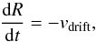$\frac{\mathrm{d}\mathit{R}}{\mathrm{d}\mathit{t}}\mathrm{=}\mathrm{-}{\mathit{v}}_{\mathrm{drift}}\mathit{,}$(36)with the drift velocity a function of Ωt_s. Assuming a fixed dust to gas ratio of 10^-2 throughout the disk, we can solve Eqs. (35) and (36) to obtain the evolution of the vertically integrated peak mass. Catastrophic fragmentation is taken into account by setting (dm_p/ dt) = 0 when v_turb>v_frag for two particles of mass m_p. Figure 13 shows lines along which the dust evolves, starting from m = m₀ at various locations in the disk. The left plot shows the results for compact growth (i.e., φ = 1 at all times), after 10⁶ yr. (For the compact case, we have temporarily set v_frag = 10 m s^-1.) Initially, growing aggregates are not moving radially, resulting in vertical lines in Fig. 13. As the particles’ Stokes numbers increase, collision velocities and drift speeds increase. In the inner regions of the disk, the maximum size is limited by fragmentation through same-sized collisions. Particles cannot grow larger than ~cm, and will inevitably drift inwards. In the intermediate region, from 20−100 AU, the fragmentation velocity is not reached. Here, the maximum size is set by radial drift. In the outermost disk (beyond 10² AU), growth is very slow because of the low dust densities, and 10⁶ yr is not enough to reach the size necessary to start drifting. The general behavior is identical to what is observed in full compact coagulation models (see Fig. 3 in Testi et al. 2014).

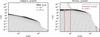Fig. 13 Evolution of mp(t) and R(t) for dust coagulation as obtained from the semi-analytical model (Eqs. (35) and (36)), for an MMSN disk and α = 10-3. Lines indicate different starting conditions R(t = 0), and are evolved for 106 yrs. Left: compact growth: φ = 1 at all times, and vfrag = 10 m s-1. Right: porous growth: the internal structure of the aggregates is set by hit and stick growth, followed by collisional compaction or gas and self-gravity compaction. Gray lines have no erosion, while black lines show the results for veros = 40 m s-1. Colored lines and ⊚-symbols indicate the evolution and steady state peak mass obtained through local MC simulations (Sect. 4.2).

The gray lines in the right-hand panel of Fig. 13 show the results of the semi-analytical model for porous growth, where φ is set by collisional, gas pressure, and self-gravity compaction, assuming perfect sticking. Since we are assuming the m_p particles carry the total dust mass, we do not have any information about the mass-distribution of smaller particles. Nonetheless, we can mimic the effect of effective erosion, by setting (dm_p/ dt) = 0 when the relative velocity between the mass dominating particle and small projectiles (taken to be monomers) exceeds v_eros. The black solid lines in the right panel of Fig. 13 show the results for v_eros = 40 m s^-1, while the red lines indicate results for the peak mass of the full MC models for the same erosion threshold velocity (although that the maximum mass reached in these models can be a factor of ~10 larger). We have also included a full model run at 200 AU, which we evolved for 10⁶ yrs. The results of the semi-analytical model agree with the simulations of the previous section remarkably well.

6. Discussion

From the maximum sizes fluffy aggregates can reach at a given location, we identify three zones in the protoplanetary disk:

• 3−10 AU: assuming perfect sticking, the combination of Stokes drag and enhanced collisional cross sections allows the porous aggregates in the inner disk to out-grow the radial drift barrier, and reach planetesimal sizes without experiencing significant drift. However, when erosion is efficient, mass loss in erosive collisions stalls the growth around Ωt_s ~ 1, preventing the porous aggregates from crossing the radial drift barrier (Fig. 11).

• 10−100 AU: at intermediate radii growth timescales increase and radial drift takes over, even before aggregates reach sizes and stopping times that allow erosive collisions to take place.

• >100 AU: in the outer disk, the disk lifetime is not long enough for particles to grow to sizes where significant drift occurs. In the porous growth scenario, aggregates this far out are in the hit-and-stick regime, and their surface-to-mass ratio does not change when they gain mass. As a result, hardly any drift is visible. In the compact case, an increase in mass automatically results in a decrease in the surface-to-mass ratio, and the onset of radial drift is already visible for very low particle masses.

For erosion to start, the collision velocity between target and projectile needs to exceed v_eros. In the limit where the projectiles are monomers that couple to the gas extremely well, this collision velocity equals the relative velocity of the large bodies with respect to the gas. When the largest particle has Ωt_s ≫ 1, it moves on a Keplerian orbit, and v_dg ≃ ηv_K, while bodies with Ωt_s = 1 have a slightly larger velocity with respect to the gas (Weidenschilling 1977). For the disk model employed in this work (Sect. 2.1), the quantity ηv_K does not depend on R, and thus the maximum drift speed is constant though out the disk. It is clear then from Eq. (33) that growing aggregates in colder disks (lower c_s), or disks with a (locally) shallower gas density profile might suffer less from erosion.

It is clear from Fig. 11 that the size of v_eros is an essential parameter: its value, together with ηv_K, determines whether growth beyond Ωt_s = 1 is possible or not. Unfortunately, the value of v_eros, or even its relation to v_frag, is not accurately known for the large and highly-porous icy bodies in question (Sect. 2.3.3). Numerical investigations, showing conflicting trends for erosion efficiency with mass ratio, often employ monodisperse grain sizes (e.g., Seizinger et al. 2013; Wada et al. 2013), and the threshold velocities depend almost linearly on the grain radius (Eq. (12)), a parameter which itself is not well constrained. At the same time, the only available experimental work on erosion for ices used a distribution of grain sizes (Gundlach & Blum 2014). In addition, both numerical and experimental studies are restricted to sizes ≲ mm and porosities ≳ 10^-1, and cover a soberingly small portion of the parameter space encountered in this work (e.g., Fig. 8). Future studies, numerical as well as experimental, are encouraged to elucidate these matters, and constrain the threshold for erosion and its dependence on target/projectile sizes and porosity. Finally, we assume that material that is eroded locally is removed from the target. In reality, the fate of the fragments will be determined by the local gas flow and the velocity with which they are ejected. For very porous targets, the gas flow through and around the surface of the target might result in these fragments being re-accreted (Wurm et al. 2004). If efficient, this re-accretion might be a way to alleviate the destructive influence of erosive collisions. On the other hand, the flow through a body is likely to be insignificant, unless it is extremely porous (Sekiya & Takeda 2005).

So far we have assumed that while erosion can play an important role, catastrophic fragmentation does not occur. The maximum velocity between same-sized bodies is reached for Ωt_s = 1, and equals ~(3/2)α^1/2c_s (Eq. (11)). Since the sound speed diminishes for increasing radii, this velocity is highest in the inner disk. For typical turbulence strengths (α ≲ 10^-3) and small icy monomers, this velocity will not exceed the fragmentation threshold velocity (Eq. (12)), and, especially in the outer disk, fragmentation of icy bodies through catastrophic fragmentation is very unlikely. However, if all collisions result in sticking, small particles (≲ 100 μm) are removed from the protoplanetary nebula very rapidly, contradicting observational constraints (Dullemond & Dominik 2005; Dominik & Dullemond 2008). Drift-induced erosion can alleviate these issues, since the maximum drift velocity is high throughout the entire disk.

In this work, we have assumed collisions below the fragmentation threshold to result in perfect sticking, i.e., the mass of the resulting aggregate equals the sum of both colliding masses. However, even for collisions below the fragmentation threshold velocity, a significant amount of mass may be ejected during a collision, especially if the collision occurs at a large impact parameter (Paszun & Dominik 2009; Wada et al. 2013). An advantage of a MC model approach like the one presented here, is that it is relatively straightforward to include an additional random number to determine, for example, the impact parameter. The difficulty lies in obtaining a collision model that describes the collisional outcome as a function of this parameter. A good start would be the work of Wada et al. (2013), who show the growth efficiency as a function of impact parameter (Fig. 4). Basically, head-on collisions promote growth, while collisions with a large impact parameter result in little mass gain. Unfortunately, much less is known about the porosities of the resulting aggregates.

At the heart of the model of Sect. 3 lies the assumption that an aggregate is adequately described by two quantities: its mass and (average) porosity. While this represents a considerable improvement on the compact coagulation assumption, a single average porosity does not allow a complex internal structure of the aggregates. For small grains, the accuracy of this assumption will depend on their collisional history. For example, one can imagine a porous aggregate with a denser outer shell being formed if the aggregate is compacted through many collisions with small mass ratios (Meisner et al. 2012). Such a compact rim will hardly alter the aggregate’s average porosity, but can influence its sticking and erosion behavior (Schräpler & Blum 2011). Likewise, gas- and self-gravity compaction need not result in a homogenous internal structure. With instruments such as CONCERT on board ESA’s Rosetta and Philae capable of probing the internal structure of large solar system objects, studies focussing on the internal structure of the larger bodies, as determined by its growth and compaction history would be very interesting. The MC method developed in this paper would be suitable for such studies, since adding parameters describing the aggregates is relatively straightforward.

6.1. Future work and implications

6.1.1. Pebble accretion

A novel idea in the field of planet formation is the process of pebble accretion, where protoplanets grow very efficiently by accreting small pebbles (Ormel & Klahr 2010; Lambrechts & Johansen 2012, 2014; Kretke & Levison 2014). These models rely on the radial influx of particles drifting in from the outer disk. As in the compact case, porous growth leads to the creation of rapidly drifting bodies in the region between 10 and 10² AU (Fig. 13). While the Stokes numbers of these particles are similar to the drifting pebbles in the compact case, their masses, sizes, and porosities can differ by many orders of magnitude (see also Fig. 14). In addition, the drag regime that the drifting bodies experience differs from the compact case (Fig. 1). Future studies are needed to address the effect of these factors on the efficiency of pebble accretion.

Fig. 14 Same as the right-hand plot of Fig. 13, but with aggregate size on the vertical axis.

6.1.2. Streaming instability

While – depending on the critical erosion velocity – rapid coagulation into masses as large as planetesimals might be prevented by erosive collisions, the conditions created by this process might be favorable for triggering planetesimal formation by streaming instability (Youdin & Goodman 2005; Johansen et al. 2007; Bai & Stone 2010a,b). To trigger streaming instability, the majority of mass needs to reside in particles with high Stokes numbers; the midplane dust to gas ratio has to be close to unity; and the local vertically integrated dust-to-gas ratio needs to exceed ~0.03 (Dra¸żkowska & Dullemond 2014). The first two conditions can be studied with simulations like the ones presented in this work. For example, for the steady-state distribution reached for v_eros = 40 m s^-1 at 5 AU for α = 10^-3, approximately 50% of the dust mass resides in particles with Ωt_s> 10^-2, and the midplane dust-to-gas ratio is ~10^-1. For weaker turbulence, the midplane dust-to-gas ratio will be increased further, since h_d ~ α^1/2 (Eq. (6)). Because our simulations are local, the vertically integrated dust-to-gas ratio stays constant at 10^-2. To fulfill the third condition, the dust-to-gas ratio either has to be larger from the beginning, or must increase by material drifting in from the outer disk. To study this, a global model is required, that calculates the evolution of the dust surface density in the presence of radial drift and erosion. In conclusion, drift-induced erosion appears to be a robust way of concentrating mass around Ωt_s ~ 1, and is expected to create conditions favorable for streaming instability.

6.1.3. The breakthrough case

For compact silicate bodies in the inner disk, bouncing and fragmentation are very effective in stopping growth at mm-cm sizes. The breakthrough scenario, in which a small number of lucky particles still manages to gain mass, might render further growth possible (Windmark et al. 2012; Garaud et al. 2013). The total mass fraction of these lucky particles can be extremely small, making this a challenging process to model for both differential and MC methods (Dra¸żkowska et al. 2014). The distribution method used in this work, as outlined in Sect. 3.3, is capable of resolving the entire mass distribution, including parts that contribute very little to the total dust mass, and appears to be suitable for studying the breakthrough case.

6.1.4. Opacities of porous grains

The optical properties of dust distributions resulting from porous growth are very different from populations containing exclusively solid particles. Not only are the mass distributions themselves different (e.g., Fig. 13), but also the scattering and absorption opacities of the individual grains are affected significantly by porosity (Kataoka et al. 2014; Cuzzi et al. 2014). For simple dust mass distributions, the effect of grain porosity on the appearance of protoplanetary disks has been investigated by Kirchschlager & Wolf (2014). Combining self-consistent coagulation models - including erosion and fragmentation – with porosity-dependent dust opacities will reveal the full impact porous growth has on the appearance of protoplanetary disks.

7. Conclusions

Porous growth is very different from compact growth (Fig. 13). For example, porous particles have larger collisional cross sections than compact particles of the same mass. More importantly, the aerodynamical properties of porous aggregates can differ greatly from those of compact particles (Fig. 1), causing differences in relative velocities (Fig. 2), vertical settling, and radial drift.

We have modeled the coagulation of porous icy particles in the outer parts of protoplanetary disks, tracing the evolution of the mass and filling factor of the individual aggregates in time. We consider compaction through collisions, gas pressure, and self-gravity (Fig. 8), and include a physical model for erosive collisions (Sects. 2.3.2 and 2.3.3). The main findings of this work are:

• 1.

  Porous icy aggregates can outgrow the radial drift barrier in the inner ~10 AU, despite increased growth timescales resulting from gas- and self-gravity compaction, if the perfect sticking assumption holds (Figs. 7 and 13). This is in agreement with Okuzumi et al. (2012) and Kataoka et al. (2013b).

• 2.

  While the maximum collision velocity between similar particles (~ α^1/2c_s) typically does not exceed the critical fragmentation threshold velocity for icy bodies, the velocity between drifting aggregates (with Ωt_s ≥ 1) and smaller bodies is much larger (~ ηv_K), and can exceed the critical threshold velocity for erosion (Fig. 2).

• 3.

  In these cases, we find that the mass loss through erosive collisions can balance the growth through same-size collisions, halting the growth of the largest bodies (Figs. 10 and 11). In our local simulations, this results in a steady-state where the largest bodies have Ωt_s ~ 1, and the porosity of the small fragment distribution is dominated by the fact that all fragments have at some point been part of these large eroded particles (Figs. 9 and 12). Only for the highest erosion threshold velocity we considered (v_eros = 60 m s^-1) do the aggregates with Ωt_s ~ 1 manage to gain mass and grow through the drift barrier.

• 4.

  A simple semi-analytical model (Sect. 5) accurately describes the growth and drift behavior of the mass-dominating bodies. While no information is obtained about the dust mass distribution, such an approach is very useful for investigating how the size of the largest bodies depends on disk parameters such as the total disk mass, turbulence strength, and dust-to-gas ratio, or aggregate properties such as monomer size and erosion/fragmentation threshold velocities.

Acknowledgments

Dust studies at Leiden Observatory are supported through the Spinoza Premie of the Dutch science agency, NWO. S.K. would like to thank C.P. Dullemond, J. Dra¸żkowska and T. Birnstiel for useful discussions, and S. Okuzumi for comments and helping with the comparison to his work. The authors thank B. Gundlach and J. Blum for sharing a version of their manuscript. C.W.O. acknowledges support for this work by NASA through Hubble Fellowship grant No. HST-HF-51294.01-A awarded by the Space Telescope Science Institute, which is operated by the Association of Universities for Research in Astronomy, Inc., for NASA, under contract NAS 5-26555.

References

All Figures

Fig. 1 Particle Stokes numbers as a function of mass, in the midplane of an MMSN disk at 5 AU. Different lines show compact particles (red), porous aggregates with constant φ = 104 (yellow), and aggregates with a constant fractal dimension of 2.5 (green). For the solid lines, all drag regimes (Epstein, Stokes and Newton) have been taken into account, while the dashed lines indicate the results using only Epstein and Stokes drag. Horizontal lines indicate Ωts = 1 (where drift is fastest) and Ωts = α = 10-3 (where particles start to settle to the midplane).

In the text

Fig. 2 Relative velocities between compact (left) or very porous (right) particles with masses mi and mj at the midplane of an MMSN-disk at 5 AU with α = 10-3. The masses range from single monomers to aggregates containing 1032 monomers. The contours give relative velocities in m s-1, and the colors indicate the dominating source for the relative velocity: Brownian motion (BrM), turbulence (Trb), settling (Set), radial drift (Rad), or azimuthal drift (Azi). Epstein, Stokes, and Newton drag regimes have been taken into account.

In the text

	Fig. 3 a) Schematic of a collision between unequal particles with a mass ratio R(m) = (mproj/mtarget) ≪ 1. b) Sticking occurs when vrel<veros. The mass of the projectile is added to the target. c) Collisions above the erosion threshold velocity lead to erosion. The mass loss of the target is given by the erosion efficiency ϵeros and the mass of the projectile.
In the text

	Fig. 4 Evolution of the normalized particle mass distribution at 5 AU with α = 10-3, assuming perfect sticking and without compaction through gas and self-gravity. Only Epstein are Stokes drag are considered. Solid lines indicate averages over 4 MC runs with identical starting conditions, and the shaded areas represent a spread of 1σ.
In the text

	Fig. 5 Like Fig. 4, but with compaction through gas and self-gravity and Newton drag for particles with Rep> 1.
In the text

	Fig. 6 Evolution of the growth- and radial drift timescale of the peak mass for the perfect sticking model at 5 AU with α = 10-3. The dotted line indicates (tdrift/ 30). Only collisional compaction has been taken into account.
In the text

	Fig. 7 Evolution of the growth- and radial drift timescale of the peak mass for the perfect sticking model at 5 AU with α = 10-3. The dotted line indicates (tdrift/ 30). Compaction from gas and self-gravity, and Newton drag have been taken into account.
In the text

Fig. 8 Evolution of the internal structure of the mass-dominating particles, for the perfect sticking models at 5 AU, for the models with and without non-collisional compaction mechanisms. Aggregates start out as monomers in the top left corner, and grow towards larger sizes and porosities. Lines show individual simulations. Open symbols correspond to points where the mass dominating particles reach a = λmfp (°); ts = tη (◇); Ωts = α (▿); and Ωts = 1 (□). Filled symbols show peak mass and filling factor at the times of first: collisional compaction (⋆); gas-pressure compaction (◆); and self-gravity compaction (•).

In the text

	Fig. 9 Evolution of the normalized particle mass distribution at 5 AU with α = 10-3, assuming veros = 20 m s-1. The full compaction model is used.
In the text

Fig. 10 Projectile distribution mass functions for simulation E1, constructed for the maximum masses (mt =•) at various times. Colors and times correspond to Fig. 9. For each distribution, the stopping time of the mt-particle is given, and the weights of the total positive and negative area are plotted. The distributions have been normalized in such a way, that the absolute sum of the contributions equals 1.

In the text

	Fig. 11 Evolution of ζ(mmax) for erosive simulations with veros = 20,40,60 m s-1 as a function of Ωts(mmax), showing the impact of erosion on the ability of the largest bodies to grow. In the upper two panels, the steady-state is indicated by the ⊚-symbol.
In the text

	Fig. 12 Masses and filling factors of all unique families at different times, for simulation E1. One dot corresponds to one family, and does not provide information about the total mass or number of members in that family.
In the text

Fig. 13 Evolution of mp(t) and R(t) for dust coagulation as obtained from the semi-analytical model (Eqs. (35) and (36)), for an MMSN disk and α = 10-3. Lines indicate different starting conditions R(t = 0), and are evolved for 106 yrs. Left: compact growth: φ = 1 at all times, and vfrag = 10 m s-1. Right: porous growth: the internal structure of the aggregates is set by hit and stick growth, followed by collisional compaction or gas and self-gravity compaction. Gray lines have no erosion, while black lines show the results for veros = 40 m s-1. Colored lines and ⊚-symbols indicate the evolution and steady state peak mass obtained through local MC simulations (Sect. 4.2).

In the text

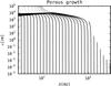	Fig. 14 Same as the right-hand plot of Fig. 13, but with aggregate size on the vertical axis.
In the text

References

- Bai, X.-N., & Stone, J. M. 2010a, ApJ, 722, 1437 [NASA ADS] [CrossRef] [Google Scholar]
- Bai, X.-N., & Stone, J. M. 2010b, ApJ, 722, L220 [NASA ADS] [CrossRef] [Google Scholar]
- Birnstiel, T., Dullemond, C. P., & Brauer, F. 2010, A&A, 513, A79 [NASA ADS] [CrossRef] [EDP Sciences] [Google Scholar]
- Blum, J., & Wurm, G. 2008, ARA&A, 46, 21 [NASA ADS] [CrossRef] [EDP Sciences] [Google Scholar]
- Cuzzi, J. N., Estrada, P. R., & Davis, S. S. 2014, ApJS, 210, 21 [NASA ADS] [CrossRef] [Google Scholar]
- Dominik, C., & Dullemond, C. P. 2008, A&A, 491, 663 [NASA ADS] [CrossRef] [EDP Sciences] [Google Scholar]
- Dominik, C., & Tielens, A. G. G. M. 1995, Philosophical Magazine, Part A, 72, 783 [Google Scholar]
- Dominik, C., & Tielens, A. G. G. M. 1997, ApJ, 480, 647 [NASA ADS] [CrossRef] [Google Scholar]
- Drążkowska, J., & Dullemond, C. P. 2014, A&A, 572, A78 [NASA ADS] [CrossRef] [EDP Sciences] [Google Scholar]
- Drążkowska, J., Windmark, F., & Dullemond, C. P. 2014, A&A, 567, A38 [NASA ADS] [CrossRef] [EDP Sciences] [Google Scholar]
- Dullemond, C. P., & Dominik, C. 2005, A&A, 434, 971 [NASA ADS] [CrossRef] [EDP Sciences] [Google Scholar]
- Garaud, P., Meru, F., Galvagni, M., & Olczak, C. 2013, ApJ, 764, 146 [NASA ADS] [CrossRef] [Google Scholar]
- Gillespie, D. T. 1975, J. Atmos. Sci., 32, 1977 [NASA ADS] [CrossRef] [Google Scholar]
- Gundlach, B., & Blum, J. 2014, ApJ, accepted [Google Scholar]
- Gundlach, B., Kilias, S., Beitz, E., & Blum, J. 2011, Icarus, 214, 717 [NASA ADS] [CrossRef] [Google Scholar]
- Güttler, C., Blum, J., Zsom, A., Ormel, C. W., & Dullemond, C. P. 2010, A&A, 513, A56 [NASA ADS] [CrossRef] [EDP Sciences] [Google Scholar]
- Haisch, Jr., K. E., Lada, E. A., & Lada, C. J. 2001, ApJ, 553, L153 [NASA ADS] [CrossRef] [Google Scholar]
- Hayashi, C. 1981, Prog. Theor. Phys. Suppl., 70, 35 [NASA ADS] [CrossRef] [MathSciNet] [Google Scholar]
- Johansen, A., Oishi, J. S., Mac Low, M.M., et al. 2007, Nature, 448, 1022 [Google Scholar]
- Johansen, A., Blum, J., Tanaka, H., et al. 2014, in Protostars and Planets VI, University of Arizona Press, eds. H. Beuther, et al., in press [arXiv:1402.1344] [Google Scholar]
- Kataoka, A., Tanaka, H., Okuzumi, S., & Wada, K. 2013a, A&A, 557, L4 [NASA ADS] [CrossRef] [EDP Sciences] [Google Scholar]
- Kataoka, A., Tanaka, H., Okuzumi, S., & Wada, K. 2013b, A&A, 554, A4 [NASA ADS] [CrossRef] [EDP Sciences] [Google Scholar]
- Kataoka, A., Okuzumi, S., Tanaka, H., & Nomura, H. 2014, A&A, 568, A42 [NASA ADS] [CrossRef] [EDP Sciences] [Google Scholar]
- Kempf, S., Pfalzner, S., & Henning, T. K. 1999, Icarus, 141, 388 [NASA ADS] [CrossRef] [Google Scholar]
- Kirchschlager, F., & Wolf, S. 2014, A&A, 568, A103 [NASA ADS] [CrossRef] [EDP Sciences] [Google Scholar]
- Kothe, S., Güttler, C., & Blum, J. 2010, ApJ, 725, 1242 [NASA ADS] [CrossRef] [Google Scholar]
- Kretke, K. A., & Levison, H. F. 2014, AJ, 148, 109 [NASA ADS] [CrossRef] [Google Scholar]
- Krijt, S., Güttler, C., Heißelmann, D., Dominik, C., & Tielens, A. G. G. M. 2013, J. Phys. D Appl. Phys., 46, 5303 [Google Scholar]
- Krijt, S., Dominik, C., & Tielens, A. G. G. M. 2014, J. Phys. D Appl. Phys., 47, 175302 [Google Scholar]
- Lambrechts, M., & Johansen, A. 2012, A&A, 544, A32 [Google Scholar]
- Lambrechts, M., & Johansen, A. 2014, A&A, 572, A107 [NASA ADS] [CrossRef] [EDP Sciences] [Google Scholar]
- Meisner, T., Wurm, G., & Teiser, J. 2012, A&A, 544, A138 [NASA ADS] [CrossRef] [EDP Sciences] [Google Scholar]
- Mukai, T., Ishimoto, H., Kozasa, T., Blum, J., & Greenberg, J. M. 1992, A&A, 262, 315 [NASA ADS] [Google Scholar]
- Nakagawa, Y., Sekiya, M., & Hayashi, C. 1986, Icarus, 67, 375 [NASA ADS] [CrossRef] [Google Scholar]
- Okuzumi, S., Tanaka, H., & Sakagami, M.-A. 2009, ApJ, 707, 1247 [NASA ADS] [CrossRef] [Google Scholar]
- Okuzumi, S., Tanaka, H., Takeuchi, T., & Sakagami, M.-A. 2011, ApJ, 731, 95 [NASA ADS] [CrossRef] [Google Scholar]
- Okuzumi, S., Tanaka, H., Kobayashi, H., & Wada, K. 2012, ApJ, 752, 106 [NASA ADS] [CrossRef] [Google Scholar]
- Ormel, C. W., & Cuzzi, J. N. 2007, A&A, 466, 413 [NASA ADS] [CrossRef] [EDP Sciences] [Google Scholar]
- Ormel, C. W., & Klahr, H. H. 2010, A&A, 520, A43 [NASA ADS] [CrossRef] [EDP Sciences] [Google Scholar]
- Ormel, C. W., & Spaans, M. 2008, ApJ, 684, 1291 [NASA ADS] [CrossRef] [EDP Sciences] [Google Scholar]
- Ormel, C. W., Spaans, M., & Tielens, A. G. G. M. 2007, A&A, 461, 215 [NASA ADS] [CrossRef] [EDP Sciences] [Google Scholar]
- Paszun, D., & Dominik, C. 2008, A&A, 484, 859 [NASA ADS] [CrossRef] [EDP Sciences] [Google Scholar]
- Paszun, D., & Dominik, C. 2009, A&A, 507, 1023 [NASA ADS] [CrossRef] [EDP Sciences] [Google Scholar]
- Poppe, T., Blum, J., & Henning, T. 2000, ApJ, 533, 454 [NASA ADS] [CrossRef] [Google Scholar]
- Schräpler, R., & Blum, J. 2011, ApJ, 734, 108 [NASA ADS] [CrossRef] [Google Scholar]
- Seizinger, A., & Kley, W. 2013, A&A, 551, A65 [NASA ADS] [CrossRef] [EDP Sciences] [Google Scholar]
- Seizinger, A., Krijt, S., & Kley, W. 2013, A&A, 560, A45 [NASA ADS] [CrossRef] [EDP Sciences] [Google Scholar]
- Sekiya, M., & Takeda, H. 2005, Icarus, 176, 220 [NASA ADS] [CrossRef] [Google Scholar]
- Shakura, N. I., & Sunyaev, R. A. 1973, A&A, 24, 337 [NASA ADS] [Google Scholar]
- Suyama, T., Wada, K., & Tanaka, H. 2008, ApJ, 684, 1310 [NASA ADS] [CrossRef] [Google Scholar]
- Suyama, T., Wada, K., Tanaka, H., & Okuzumi, S. 2012, ApJ, 753, 115 [NASA ADS] [CrossRef] [Google Scholar]
- Testi, L., Birnstiel, T., Ricci, L., et al. 2014, in Protostars and Planets VI, University of Arizona Press, eds. H. Beuther, et al., in press [arXiv:1402.1354] [Google Scholar]
- Tielens, A. G. G. M., McKee, C. F., Seab, C. G., & Hollenbach, D. J. 1994, ApJ, 431, 321 [NASA ADS] [CrossRef] [Google Scholar]
- Wada, K., Tanaka, H., Suyama, T., Kimura, H., & Yamamoto, T. 2007, ApJ, 661, 320 [NASA ADS] [CrossRef] [Google Scholar]
- Wada, K., Tanaka, H., Suyama, T., Kimura, H., & Yamamoto, T. 2009, ApJ, 702, 1490 [NASA ADS] [CrossRef] [Google Scholar]
- Wada, K., Tanaka, H., Suyama, T., Kimura, H., & Yamamoto, T. 2011, ApJ, 737, 36 [NASA ADS] [CrossRef] [Google Scholar]
- Wada, K., Tanaka, H., Okuzumi, S., et al. 2013, A&A, 559, A62 [NASA ADS] [CrossRef] [EDP Sciences] [Google Scholar]
- Weidenschilling, S. J. 1977, MNRAS, 180, 57 [NASA ADS] [CrossRef] [Google Scholar]
- Weidenschilling, S. J. 1980, Icarus, 44, 172 [NASA ADS] [CrossRef] [Google Scholar]
- Whipple, F. L. 1972, in From Plasma to Planet, ed. A. Elvius, 211 [Google Scholar]
- Windmark, F., Birnstiel, T., Ormel, C. W., & Dullemond, C. P. 2012, A&A, 544, L16 [NASA ADS] [CrossRef] [EDP Sciences] [Google Scholar]
- Wurm, G., Paraskov, G., & Krauss, O. 2004, ApJ, 606, 983 [NASA ADS] [CrossRef] [Google Scholar]
- Wurm, G., Paraskov, G., & Krauss, O. 2005, Icarus, 178, 253 [NASA ADS] [CrossRef] [MathSciNet] [Google Scholar]
- Youdin, A. N., & Goodman, J. 2005, ApJ, 620, 459 [NASA ADS] [CrossRef] [Google Scholar]
- Youdin, A. N., & Lithwick, Y. 2007, Icarus, 192, 588 [NASA ADS] [CrossRef] [Google Scholar]
- Zsom, A., & Dullemond, C. P. 2008, A&A, 489, 931 [NASA ADS] [CrossRef] [EDP Sciences] [Google Scholar]
- Zsom, A., Ormel, C. W., Güttler, C., Blum, J., & Dullemond, C. P. 2010, A&A, 513, A57 [NASA ADS] [CrossRef] [EDP Sciences] [Google Scholar]