| Issue |
A&A
Volume 574, February 2015
|
|
|---|---|---|
| Article Number | A105 | |
| Number of page(s) | 14 | |
| Section | Extragalactic astronomy | |
| DOI | https://doi.org/10.1051/0004-6361/201424711 | |
| Published online | 03 February 2015 | |
The evolution of galaxy star formation activity in massive haloes⋆
1 Excellence Cluster Universe, Boltzmannstr. 2, 85748 Garching, Germany
e-mail: This email address is being protected from spambots. You need JavaScript enabled to view it.
2 Max-Planck-Institut für Extraterrestrische Physik (MPE), Postfach 1312, 85741 Garching, Germany
3 INAF – Osservatorio Astronomico di Trieste, via G.B. Tiepolo 11, 34143 Trieste, Italy
4 INAF – Osservatorio Astronomico di Bologna, via Ranzani 1, 40127 Bologna, Italy
5 Dipartimento di Astronomia, Università di Bologna, via Ranzani 1, 40127 Bologna, Italy
6 Dipartimento di Astronomia, Università di Padova, Vicolo dell’Osservatorio 3, 35122 Padova, Italy
7 Laboratoire AIM, CEA/DSM-CNRS-Université Paris Diderot, IRFU/Service d’Astrophysique, Bât. 709, CEA-Saclay, 91191 Gif-sur-Yvette Cedex, France
8 National Optical Astronomy Observatory, 950 North Cherry Avenue, Tucson, AZ 85719, USA
9 Herschel Science Centre, European Space Astronomy Centre, ESA, Villanueva de la Cañada, 28691 Madrid, Spain
10 NASA Herschel Science Center, Caltech 100-22, Pasadena, CA 91125, USA
11 Institute for Astronomy 2680 Woodlawn Drive Honolulu, HI 96822-1897, USA
12 IPAC, Caltech 100-22, Pasadena, CA 91125, USA
Received: 30 July 2014
Accepted: 13 October 2014
Abstract
Context. There is now a large consensus that the current epoch of the cosmic star formation history (CSFH) is dominated by low mass galaxies while the most active phase, between redshifts 1 and 2, is dominated by more massive galaxies, which evolve more quickly.
Aims. Massive galaxies tend to inhabit very massive haloes, such as galaxy groups and clusters. We aim to understand whether the observed “galaxy downsizing” could be interpreted as a “halo downsizing”, whereas the most massive haloes, and their galaxy populations, evolve more rapidly than the haloes with lower mass.
Methods. We studied the contribution to the CSFH of galaxies inhabiting group-sized haloes. This is done through the study of the evolution of the infra-red (IR) luminosity function of group galaxies from redshift 0 to redshift ~1.6. We used a sample of 39 X-ray-selected groups in the Extended Chandra Deep Field South (ECDFS), the Chandra Deep Field North (CDFN), and the COSMOS field, where the deepest available mid- and far-IR surveys have been conducted with Spitzer MIPS and with the Photodetector Array Camera and Spectrometer (PACS) on board the Herschel satellite.
Results. Groups at low redshift lack the brightest, rarest, and most star forming IR-emitting galaxies observed in the field. Their IR-emitting galaxies contribute ≤10% of the comoving volume density of the whole IR galaxy population in the local Universe. At redshift ≳1, the most IR-luminous galaxies (LIRGs and ULIRGs) are mainly located in groups, and this is consistent with a reversal of the star formation rate (SFR) vs. density anti-correlation observed in the nearby Universe. At these redshifts, group galaxies contribute 60–80% of the CSFH, i.e. much more than at lower redshifts. Below z ~ 1, the comoving number and SFR densities of IR-emitting galaxies in groups decline significantly faster than those of all IR-emitting galaxies.
Conclusions. Our results are consistent with a “halo downsizing” scenario and highlight the significant role of “environment” quenching in shaping the CSFH.
Key words: galaxies: evolution / galaxies: clusters: general / galaxies: luminosity function, mass function / galaxies: groups: general
Herschel is an ESA space observatory with science instruments provided by European-led Principal Investigator consortia and with important participation from NASA.
© ESO, 2015
1. Introduction
One of the most fundamental correlations between the properties of galaxies in the local Universe is the so-called morphology-density relation. Since the early work of Dressler (1980), a plethora of studies utilizing multi-wavelength tracers of activity have shown that late type star-forming galaxies favour low-density regimes in the local Universe (e.g. Gómez et al. 2003). In particular, the cores of massive galaxy clusters are galaxy graveyards of massive spheroidal systems dominated by old stellar populations. Much of the current debate centres on whether the relation arises early on during the formation of the object, or whether it is caused by environment-driven evolution. However, as we approach the epoch when the quiescent behemoths should be forming the bulk of their stars at z ≳ 1.5 (e.g. Rettura et al. 2010), the relation between star formation (SF) activity and environment should progressively reverse. Elbaz et al. (2007) and Cooper et al. (2008) observe the reversal of the star formation rate (SFR) vs. density relation already at z ~ 1 in the GOODS and the DEEP2 fields, respectively. Using Herschel PACS data, Popesso et al. (2011) show that the reversal is mainly observed in high-mass galaxies and is due to a higher fraction of active galactic nuclei (AGN), which exhibit slightly higher SFR than galaxies of the same stellar mass (Santini et al. 2012). On the other hand, Feruglio et al. (2010) find no reversal in the COSMOS field and argue that the reversal, if any, must occur at z ~ 2. Similarly, Ziparo et al. (2014) find that the local anti-correlation tends to flatten towards high redshift rather than reversing.
On a related topic, there is now a large consensus that the cosmic star formation history (CSFH) peaks at increasingly higher redshifts for galaxies of higher stellar mass at redshift zero. The star formation activity of low-mass galaxies (stellar mass ≤1010 M⊙) peaks at redshift z ~ 0.2, whereas that of more massive galaxies (stellar mass ≥1011 M⊙) monotonically declines from z ~ 0.5 − 1 or higher (Heavens et al. 2004; Gruppioni et al. 2013, up to z ~ 2 for stellar mass > 1012 M⊙). This monotonic decline leads to a decrease of an order of magnitude in the SFR density of the Universe after z ~ 1. Highly star-forming galaxies such as the luminous infrared galaxies (LIRGs) are rare in the local Universe, but are the main contributors to the CSFH at z ~ 1 − 3 (Le Floc’h et al. 2005; Pérez-González et al. 2005; Caputi et al. 2007; Reddy et al. 2008; Magnelli et al. 2009, 2011, 2013). The most powerful starburst galaxies, such as the ultraluminous infrared galaxies (ULIRGs) and the sub-mm galaxies undergo the fastest evolution, dominating the CSFH only at z ~ 2–3 and disappearing, then, by redshift ~0 (Cowie et al. 2004). Most massive galaxies seem to have formed their stars early in cosmic history, and their contribution to the CSFH was significantly greater at higher redshifts through a very powerful phase of SF activity (LIRGs, ULIRGs and sub-mm galaxies). Low-mass galaxies seem to have formed much later, and they dominate the present epoch through a mild and steady SF activity. This phenomenology is generally referred to as “galaxy downsizing”. The evidence that more massive galaxies tend to reside in more massive haloes sets a clear link between the galaxy SF activity evolution and their environment. The “galaxy downsizing” scenario could therefore be interpreted in terms of a “halo downsizing” scenario as highlighted in Neistein et al. (2006) and Popesso et al. (2012).
The most straighforward way to probe whether there is a reversal of the SFR-density relation in the distant Universe and what the contribution of galaxies in massive haloes is to the CSFH is to study the evolution of the SFR density of galaxies in such haloes. In most galaxies, the bulk of UV photons, emitted by young, massive stars, is absorbed by dust and re-emitted at infrared (IR) wavelengths (see Kennicutt 1998). For this reason the IR luminosity is a very robust indicator of the bolometric output from young stars and therefore a good proxy for the galaxy SFR (e.g. Buat et al. 2002; Bell 2003). As a consequence, the evolution of the galaxy IR luminosity function (LF) provides a direct measure of the evolution of the galaxy SFR distribution.
In the local Universe the bulk of the total stellar mass is contained in galaxy groups with total mass greater than 1012.5 M⊙. The fraction of stellar mass in the more massive galaxy clusters is negligible because these are rare objects (Eke et al. 2005), and group-sized haloes are the most common high-mass haloes for a galaxy to inhabit. For this reason, we study the evolution of the IR LF of galaxies in groups, and compare it to that of more isolated field galaxies. While the IR LF of field galaxies and its evolution are relatively well known up to z ~ 2.5−3 (Caputi et al. 2007; Magnelli et al. 2009; Gruppioni et al. 2011, 2013; Reddy et al. 2008), the IR LF of galaxies in groups and clusters is still poorly known.
Most determinations of galaxy IR LFs in cluster and supercluster environments have so far been based on Spitzer data. Bai et al. (2006, 2009) analyzed the IR LFs of the rich nearby clusters Coma and A3266. According to their analysis, the bright end of the IR LF has a universal form for local rich clusters, and cluster and field IR LFs have similar values for their characteristic luminosities. Bai et al. (2009) compare the average IR LFs of these two nearby clusters and two distant (z ~ 0.8) systems and conclude that there is a redshift evolution of both the characteristic luminosity and the normalization of the LF such that higher-z clusters contain more and brighter IR galaxies. Other studies find considerable variance in the IR LF in galaxy clusters, and this might be related to the presence of substructures (Chung et al. 2010; Biviano et al. 2011).
Much less is known about the evolution of the IR LF in dark matter haloes of lower mass, such as the galaxy groups. Tran et al. (2009) determine the IR LFs in a rich galaxy cluster and four galaxy groups at z ~ 0.35. There are four times more galaxies with a high SFR in the groups than in the cluster, or equivalently, the group IR LF has an excess at the bright end relative to the cluster IR LF. On the basis of this result, Chung et al. (2010) interpret the excess of bright IR sources in the IR LF of the Bullet cluster (z ~ 0.3) as being due to the galaxy population in an infalling group (the “bullet” itself). Biviano et al. (2011) find that the IR LF of galaxies in a z ~ 0.2 large-scale filament has a bright-end excess compared to the IR LF of its neighbouring cluster. Given that the physical conditions (density, velocity dispersions) are similar in filaments and poor groups, their result appears to be consistent with Tran et al. (2009)’s.
In this paper we analyse the evolution of the group galaxy IR LF from redshift 0 to redshift z ~ 1.6 by using the newest and deepest available mid- and far-IR surveys conducted with Spitzer MIPS and with the most recent Photodetector Array Camera and Spectrometer (PACS) on board the Herschel satellite, on the major blank fields such as the Extended Chandra Deep Fields South (ECDFS), the Chandra Deep Field North (CDFN) and the COSMOS field. All these fields are part of the largest GT and KT Herschel Programmes conducted with PACS: the PACS evolutionary probe (PEP; Lutz et al. 2011) and the GOODS-Herschel Program (Elbaz et al. 2011). In addition, the blank fields considered in this work are observed extensively in the X-ray with Chandra and XMM-Newton. The ECDFS, CDFN, and COSMOS fields are also the site of extensive spectroscopic campaigns that have led to excellent spectroscopic coverage. This is essential for correctly identifying group members. We use the evolution of the group IR LF to study the SFR distribution of group galaxies and to measure their contribution to the CSFH.
The paper is structured as follows. In Sect. 2 we describe our data set. In Sect. 3 we determine the IR LF in groups. In Sect. 4 we compare the IR LF of group galaxies with the IR LF of the total population. In Sect. 5 we analyse the contribution of group galaxies to the CSFH. In Sect. 6 we compare our results with existing models of galaxy formation and evolution. In Sect. 7 we summarize our results and draw our conclusions. We adopt H0 = 70 km s-1 Mpc-1, Ωm = 0.3, ΩΛ = 0.7 throughout this paper.
2. The data set
2.1. Infrared and spectroscopic data
We use the deepest available Spitzer MIPS 24 μm and PACS 100 and 160 μm data sets for all the fields we consider in our analysis. For COSMOS these come from from the public Spitzer 24 μm (Le Floc’h et al. 2009; Sanders et al. 2007) and PEP PACS 100 and 160 μmdata (Lutz et al. 2011; Magnelli et al. 2013). Both Spitzer MIPS 24 and PEP source catalogues are obtained by applying prior extraction as described in Magnelli et al. (2009). In short, IRAC and MIPS 24 μm source positions are used to detect and extract MIPS and PACS sources, respectively. This is feasible since extremely deep IRAC and MIPS 24 μm observations are available for the COSMOS field (Scoville et al. 2007). The source extraction is based on a point-spread functioin (PSF)-fitting technique, presented in detail in Magnelli et al. (2009).
The association between 24 μmand PACS sources, at 100 and 160 μm, with their optical counterparts, taken from the optical catalogue of Capak et al. (2007) is done via a maximum likelihood method (see Lutz et al. 2011, for details). The photometric sources were cross-matched in coordinates with the sources for which a high-confidence spectroscopic redshift is available. For this purpose we use the public catalogues of spectroscopic redshifts complemented with other unpublished data. This catalogue includes redshifts from either SDSS or the public zCOSMOS-bright data acquired using VLT/VIMOS (Lilly et al. 2007, 2009) complemented with Keck/DEIMOS (PIs: Scoville, Capak, Salvato, Sanders, Kartaltepe), Magellan/IMACS (Trump et al. 2007), and MMT (Prescott et al. 2006) spectroscopic redshifts.
In the ECDFS and GOODS regions, the deepest available MIR and FIR data are provided by the Spitzer MIPS 24 μm Fidel Program (Magnelli et al. 2009) and by the combination of the PACS PEP (Lutz et al. 2011) and GOODS-Herschel (Elbaz et al. 2011) surveys at 70, 100, and 160 μm. The GOODS Herschel survey covers a smaller central portion of the entire GOODS-S and GOODS-N regions. Recently the PEP and the GOODS-H teams have combined the two sets of PACS observations to obtain the deepest ever available PACS maps (Magnelli et al. 2013) of both fields. The more extended ECDFS area has been observed in the PEP survey as well, down to a higher flux limit. As for the COSMOS catalogues, the 24 μmand PACS sources in the ECDFS and GOODS fields are associated to their optical counterparts (provided by the Cardamone et al. 2010 catalogue for ECDFS, the Santini et al. 2009 catalogue for GOODS-S, and the dedicated PEP multi-wavelength Berta et al. 2010 catalogue for GOODS-N) via a maximum likelihood method (see Lutz et al. 2011, for details). The photometric sources were cross-matched in coordinates with the sources with a high-confidence spectroscopic redshift. The redshift compilation in the ECDFS and GOODS-S region is obtained by complementing the spectroscopic redshifts contained in the Cardamone et al. (2010) catalogue with all new publicly available spectroscopic redshifts, such as the one of Silverman et al. (2010) and the Arizona ECDFS Environment Survey (ACES, Cooper et al. 2012). We clean the new compilation from redshift duplications for the same source by matching the Cardamone et al. (2010) catalogue with the Cooper et al. (2012) and the Silverman et al. (2010) catalogues within 1″ and by keeping the most accurate zspec entry (smaller error and/or higher quality flag) in case of multiple entries. With the same procedure we include the very high-quality redshifts of the GMASS survey (Cimatti et al. 2008). The spectroscopic redshift compilation for the GOODS-N region is taken from Barger et al. (2008).
Limiting fluxes in the mid- and far-IR for all fields used in this work are given in Table 1.
Properties of the PEP fields.
2.2. The X-ray selected galaxy group sample
All the blank fields considered in our analysis have been observed extensively in the X-ray with Chandra and XMM-Newton. To create a statistically significant sample of galaxy groups, we combined the X-ray selected group sample of Popesso et al. (2012) and a newly created X-ray selected group sample of the ECDFS (Ziparo et al. 2013). The sample described in Popesso et al. (2012) comprises the X-ray selected COSMOS group sample of Finoguenov et al. (in prep.) and the X-ray-detected groups of the GOODS fields. We replace, in particular, the sample of groups detected in GOODS-S with the sample of groups from the new catalogue of Ziparo et al. (2013) extracted in the larger area of the ECDFS. The data reduction of the X-ray XMM and Chandra maps of COSMOS, ECDFS, and GOODS-N were performed in a consistent way and the initial X-ray group catalogues created according to the same extended emission extraction procedure (Finoguenov et al. 2009, and in prep.). In short, the point sources were removed from the X-ray maps. The resulting “residual” image is then used to identify extended emission with at least 4σ significance with respect to the background.
As in Popesso et al. (2012) for COSMOS and GOODS-N, Ziparo et al. (2013) selected a clean subsample of groups in the ECDFS catalog with clear spectroscopic redshift identification along the line of sight, with at least ten members, the minimum required for a meaningful dynamical analysis, and without close companions, allowing for a clear definition of the spectroscopic members. This selection leads to 22 groups in the ECDFS out of the initial 50 X-ray-selected groups.
We stress that the imposition of a minimum of ten spectroscopic members is required for a secure velocity dispersion measurement, hence a secure membership definition. This selection does not lead to a bias towards rich systems in our case. Indeed, there is no magnitude or stellar mass limit imposed on the required ten members. Thus, the very high spectroscopic completeneness, in particular of GOODS-N and ECDFS (see Popesso et al. 2009; Cooper et al. 2012, for details), leads to selecting faint and very low-mass galaxy groups. Thus, if the group richness is defined as the number of galaxies brighter than a fixed absolute magnitude limit or more massive than a stellar mass limit, our sample covers a very broad range of richness values, consistent with the scatter observed in the X-ray luminosity-richness relation studied in Rykoff et al. (2012). In a forthcoming paper (Erfanianfar et al., in prep.), we will extend the current sample to groups with fewer members.
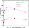 |
Fig. 1 Mean spectroscopic completeness in the Spitzer MIPS 24 μm band across all the areas of the ECDFS, GOODS-N, and COSMOS field. |
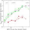 |
Fig. 2 Mean spectroscopic completeness in the Spitzer MIPS 24 μm band in the group regions as a function of the redshifts. The mean completeness is estimated for groups in different redshift bins and in different fields. The green sysmbols show the mean completeness for groups in ECDFS, magenta symbols show the mean completeness for groups in GOODS-N, and red symbols show the one for the COSMOS groups. They are grouped in three redshift bins: z< 0.4 (filled circles), 0.4 <z< 0.8 (filled triangles), and 0.8 <z< 1.2 (stars). The empy squares show the completeness in the region of the Kurk et al. (2008) structure at z ~ 1.6 in ECDFS. The mean completeness of the groups in each redshift bin is estimated in the group region within an annulus of 3 × r200 from the group centre. To guide the eye, the black dashed lines in the figure show the 24 μm flux corresponding to the LIRG limit (LIR = 1011 L⊙) at low (z ~ 0.1), intermediate (z ~ 0.5), and high (z ~ 1) redshift. The solid red line shows the 60 μJy limit used to estimate the mean group completeness. |
In all fields the total mass of the groups is derived from their X-ray luminosity (LX) by using the LX − M2001 relation of Leauthaud et al. (2010). We also impose a mass cut at M200< 2 × 10¹⁴ M⊙ to avoid including massive clusters, whose galaxy population could follow a different evolutionary path from that of groups, as shown in Popesso et al. (2012).
As a result of these selections, our group sample comprises 27 COSMOS groups at 0 <z< 0.8, 22 ECDFS groups at 0 <z< 1.0, two groups identified in the GOODS-N region at z ~ 0.85 and z ~ 1.05, and the GOODS-S group identified by Kurk et al. (2008) at z ~ 1.6. This structure was initially optically detected through the presence of an over-density of [OII] line emitters by Vanzella et al. (2006) and, then, as an over-density of elliptical galaxies by Kurk et al. (2008) in the GMASS survey. Tanaka et al. (2013) detected it as an X-ray group candidate in the ECDFS (see also Ziparo et al. 2013). The analysis of this system offers the unique opportunity to attempt to constrain the group IR LF at a very high redshift. Unlike many other systems at similar redshifts (e.g. Papovich et al. 2010), this structure does not suffer from the heavy spectroscopic bias against star forming galaxies thanks to the spectroscopic selection of red and massive galaxies, and its spectroscopic completeness is indeed high even among IR-emitting galaxies.
We restrict our sample further by selecting only those groups that reach a spectroscopic completeness in our deepest IR band, the Spitzer 24 μm band, of 60% down to 60 μJy. This flux detection threshold is reached in all fields at the 3σ level or higher.
As shown if Fig. 2, we also check for possible biases due to the spectroscopic selection function of the different fields. In particular, we check for any redshift dependence. For this purpose we estimate the spectroscopic completeness in an alternative way by using the most accurate photometric redshifts available in the considered fields. We use the photometric redshifts of Cardamone et al. 2010 in ECDFS, the one of Berta et al. 2010 for GOODS-N and the zphot of Ilbert et al. 2010 for the COSMOS field. We estimate the number of group member photometric candidates (Nzphot) as the number of MIPS detected sources in the group region (within an annulus of 3 × r200 from the group centre) and with zphot within 5 × σzphot from the group mean redshift, where σzphot is the photometric redshift uncertainty as reported in the mentioned papers. The completeness is, then, estimated as the subsample of such candidates with spectroscopic redshift and the total number Nzphot. Figure 2 shows the mean completeness for groups in different redshift bins: z< 0.4, 0.4 <z< 0.8, and 0.8 <z< 1.2. We also show the completeness estimated with this procedure for the Kurk et al. (2008) structure at z ~ 1.6. The result does not change even if we consider a smaller (3 × σzphot) or larger (10 × σzphot) photometric redshift interval for selecting the group member candidates. It is evident that there is no redshift dependence of the spectroscopic completeness. The main difference arises from the different mean spectroscopic completeness available in the different fields as already shown in Fig 1. In the ECDFS and GOODS-N fields, the spectroscopic selection captures the totality of the bright MIPS group candidates, and it ensures a very high coverage down to the 60 μJy limit. This is because all the spectroscopic selection functions are usually biased in favour of emission line galaxies and because the majority of the IR galaxies are part of this class. Thus, our requirement of a 60% spectroscopic completeness down to 60 μJy does not remove any of the groups in the ECDFS and GOODS-N. In the COSMOS field, instead, the mean completeness is lower at any MIPS flux, independently of the group redshift. For this reason, out of the initial 27 COSMOS groups, only 14 systems lie in a region of the sky with sufficient spectroscopic coverage to fulfil the selection criteria.
After this further selection, our final group sample comprises 39 groups. These are used to build composite IR LFs in different redshift bins: 0 <z< 0.4 (15 groups), 0.4 <z< 0.8 (17 groups), 0.8 <z< 1.2 (6 groups), and the z ~ 1.6 group.
In Fig. 3 we show the group masses (M200) vs. their mean redshifts. The mass-redshift distribution is rather uniform, limiting the bias againt low-mass systems at high redshift.
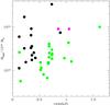 |
Fig. 3 Group masses M200 vs. mean redshifts. |
2.3. The identification of group members
The group membership is based on the Clean algorithm of Mamon et al. (2013). After selecting the main cluster peak in redshift space by the method of weighted gaps, the algorithm estimates the cluster velocity dispersion using the galaxies in the selected peak. This is then used to evaluate the virial velocity based on assumed models for the mass and velocity anisotropy profiles. These models with the estimated virial velocity are then used to predict the line-of-sight velocity dispersion of the system as a function of system-centric radius, σlos(R). Any galaxy having a rest-frame velocity within ±2.7σlos(R) at its system-centric radial distance R, is selected as a group member. We use the X-ray surface-brightness peaks as centres of the X-ray detected systems. The group members are used to re-compute the total cluster velocity dispersion, hence its virial velocity, and the procedure is iterated until convergence. The value of the virial velocity obtained at the last iteration of the Clean algorithm is used to evaluate the system dynamical mass.
As already mentioned in Popesso et al. (2012), the dynamical and X-ray mass estimates are in good agreement in the COSMOS field. As discussed in Ziparo et al. (2013), we note much less agreement for the newly defined (E)CDFS group sample, where the dynamical masses are on average higher than the X-ray masses. This could come from the ECDFS groups being on average much more distant than COSMOS groups, and this is only partially explained by the deeper X-ray exposure in the ECDFS field with respect to the COSMOS field. In the following we nevertheless use the masses derived from X-ray luminosities for all systems, since unlike dynamical masses, they do not suffer from projection effects, which may be considerable when the number of spectroscopic members is low, as in our sample. Only for the z ~ 1.6 group do we use the mass obtained by the Clean algorithm, because the X-ray luminosity is poorly estimated owing to the very low flux close to the detection level (Tanaka et al. 2013).
2.4. Bolometric IR luminosity
We use the main sequence (MS) and starburst (SB) templates of Elbaz et al. (2011) to search for the best fit to the spectral energy distribution (SED) of our group galaxies, defined by the PACS (70, 100, and 160 μm) fluxes, when available, and by the 24 μm fluxes. When the 24 μm flux is the only one available (i.e. for undetected PACS sources), we adopt the MS template, since this provides the best fit to the spectral energy distributions (SEDs) of most (80%) sources with both PACS and MIPS 24 μm detections (see for a more detailed discussion Ziparo et al. 2013). We compute the IR luminosities (LIR) by integrating the best-fit templates in the range 8–1000 μm. In principle, using the MS template for the sources with only 24 μm fluxes could cause an underestimation of the extrapolated LIR, in particular for high-redshift or for off-sequence sources, because of the higher PAHs emission of the MS template (Elbaz et al. 2011; Nordon et al. 2010). However, Ziparo et al. (2013) have shown that for the sources with PACS and 24 μm data, the LIR estimated with the best-fit templates are in good agreement with those estimated using only the 24 μm flux and the MS template ( ), with only a slight underestimation (10%) at z ≳ 1.7 and/or
  .
.
3. The galaxy group IR LF
3.1. The composite LF: method
Galaxy groups host a relatively small number of (star forming) galaxies each. As a result, the low statistics prevent us from studying the individual group LFs. The most straightforward way to overcome this problem is to consider the average LF of a statistical sample of groups or, equivalently, the composite IR LF in groups. The most widely used method of estimating a composite LF is the one of Colless (1989). In this method, the group galaxies are summed in IR luminosity bins, and the sums are scaled by the richness of the parent groups, 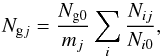 (1)where Ngj is the number of galaxies in the jth IR luminosity bin of the composite LF, Nij is the number in the jth bin of the ith IR LF in groups, Ni0 the normalization used for the ith IR LF in groups (number of group member brighter than a fixed luminosity), mj the number of groups contributing to the jth bin, and Ng0 is the sum of all the normalizations:
  (2)It is easy to note that in the Colless (1989) prescriptions, the jth bin of the composite LF represents just the mean fraction of galaxies, with respect to the normalization region, of all the groups contributing to the jth bin. In other words, Eq. (1) provides the mean fractional distribution of galaxy luminosity, multiplied by an arbitrary normalizaton, Ng0, which is just the sum of all the normalizations of the systems involved in the estimate. To obtain a composite LF with physically meaningful normalization, we rescale the mean fractional luminosity distribution,
 (3)by the mean group richness, which is the mean number of galaxies brighter than a given LIR value,
  (4)where Ngroups is the number of groups considered for the estimate of the composite IR LF. The limiting LIR value is set by the limit reached at the upper boundary of any given redshift bin, namely log LIR/L⊙ = 9,10,11, and 11.3, in the redshift bins 0–0.4, 0.4–0.8, 0.8–1.2, and at z = 1.6, respectively. In any redshift bin, groups contribute to the composite LF only down to the limiting LIR they are sampled to; that is, only the lowest z groups in any redshift bin contribute down to the bin-limiting luminosity.
Since we do not have redshifts for all galaxies in the group fields, we must correct for spectroscopic incompleteness. In principle, one should apply this correction to each IR luminosity bin by following the same method as De Propris et al. (2003) for the b band cluster LF. They estimate the spectroscopic incompleteness correction per apparent magnitude bin (corresponding to the appropriate absolute magnitude bin) for each system as the ratio between the number of all galaxies and of the galaxies with spectroscopic redshifts, in that magnitude bin. In our case this estimate is complicated by the fact that LIR is not derived from a single mid or far-IR band but from SED fitting. There is therefore not a one-to-one relation between luminosities and observed fluxes. We then adopt the following approach. We assume that the redshift determinations are unbiased with respect to group membership, and this assumption is justified by the high spatial homogeneity of the spectroscopic coverage of our fields (see for instance Cooper et al. 2012, for the ECDFS). We then take as reference photometric band the mid-IR Spitzer MIPS 24 μm band, since it is the deepest IR band in our fields. Following De Propris et al. (2003), we estimate the correction for incompleteness in the region of each group (within 2 × r200 from the group X-ray centre) per bin of MIPS 24 μm flux by assigning the following weights to each group member,  (5)where Nk is the number of galaxies in the kth 24 μm flux bin, and Nk,spec the number of galaxies in that same bin with spectroscopic determination. If all galaxies in the considered flux bin have measured redshifts, then ws,k = 1, otherwise ws,k> 1, and the galaxies with zspec also account for those without measured redshift. The mean value of ws,k in our sample is 1.5 ± 0.2, and the maximum is 2.3. To also take the photometric incompleteness in the faintest MIPS 24 μm flux bins into account, we multiply the weight ws,k by the weight wp,k that is defined as the inverse of the completeness per flux bin, estimated as described in Lutz et al. (2011). These photometric weights are wp,k ≈ 1.70, 1.25, 1.00 for sources with fluxes at the 3, 5, 8σ detection levels, respectively, corresponding to 60%, 80%, and 100% completeness, respectively. The final weight assigned to each galaxy is given by wk = ws,k × wp,k. The number of galaxies in the ith group and within the jth IR luminosity bin is then given by
  (6)where only spectroscopic members of the given group and in the given luminosity bin are considered. In the same way the normalization Ni0 of the individual IR LF in groups is obtained as the sum of wk of the group members with LIR brighter than the IR luminosity limit.
Following De Propris et al. (2003), the formal error on Ngj is obtained by propagating the errors on Nij and Ni0, which are both given by the sum in quadrature of the error of the weight wk of the contributing group members. In Eq. (5), Nk is a Poisson variable, since it is drawn from an ideal (infinite) distribution, and Nk,spec is a binomial random variable, the number of “successes” (redshift determinations) in n “trials” (number of spectroscopic targets) with probability of success, p, given by the success rate of the spectroscopic campaign. We estimate this success rate to be equal to 0.7–0.8 in the GOODS and ECDFS and COSMOS regions given the estimates reported by the major spectroscopic campaigns conducted in these fields in the redshift range considered here (Barger et al. 2008; Popesso et al. 2009; Balestra et al. 2010; Cooper et al. 2012; Lilly et al. 2009). Therefore the error on wk is given by  (7)where we neglect the contribution to the error of the photometric incompleteness weights wp,k, which turns out to be extremely stable in the simulations performed in all fields (Lutz et al. 2011; Magnelli et al. 2013). If we consider that the Poissonian error σ2(Nk) = Nk and the standard deviation of the binomial random variable Nk,spec is σ2(Nk,spec) = n × p × (1 − p) according to the standard binomial error expression, where n = Nk,spec/p, the previous equation simplifies to
  (8)
(8)
3.2. The composite LF: results
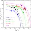 |
Fig. 4 IR LFs in galaxy groups estimated within 2 × r200 in different redshift bins: 0 <z< 0.4 (black points), 0.4 <z< 0.8 (green points), 0.8 <z< 1.2 (red points), and at z ~ 1.6 (magenta points; this is the IR LF of the structure of Kurk et al. 2008). Error bars are 1σ. The IR LF in groups in the lowest redshift bin at z< 0.1 (blue points) is obtained by averaging the IR LF in groups obtained in three different group halo mass bins by Guo et al. (2014). The solid (resp. dashed) lines, colour–coded as the points of the IR LF, indicate the best fit Schechter (resp. modified Schechter, see Saunders et al. 1990) functions. |
The composite IR LF for group galaxies is shown in Fig. 4 in the four redshift bins. In the highest redshift bin at z ~ 1.6, the IR LF is that of the Kurk et al. (2008) structure. We estimate the composite IR LF of groups within r200 and 2 × r200. Figure 4 shows, in particular, the IR LF obtained within the larger physical aperture. The LF estimated within the two apertures are consistent. We only notice that the lower statistics observed within the smaller radius (r200) leads to a slightly noisier LF, while the higher statistics obtained within the largest physical aperture (2 × r200) allow the best-fit parameters to be better constrained.
Our IR LFs do not sample the z< 0.1 redshift range. For this we use the lowest redshift determination of the IR LF of the Robotham et al. (2011) groups by Guo et al. (2014). This LF is based on the 250 μm luminosity (Lν(250 μm)) of the H-ATLAS SPIRE survey of a 135 deg2 region. In addition, we use also the LFs derived by Guo et al. (2014) in the other redshift bins (0.1–0.2, 0.2–0.3, and 0.3–0.4) to check the consistency with our LF determination in the redshift bin 0.1–0.4. For a meaningful comparison, we average the LFs obtained by Guo et al. (2014) in several group mass bins from 1012.5 to 1013 M⊙. We use as error bars the dispersion of the LF in any Lν(250 μm) luminosity bin. As a last step we use Eq. (2) of Guo et al. (2014) to transform the group Lν(250 μm) LF into the IR LF in groups.
We use three different fitting functions to find the best fit: the Schechter function, the modified Schechter function of Saunders et al. (1990), and a double power law similar to the one used by Sanders et al. (2003) for local star-forming galaxies, 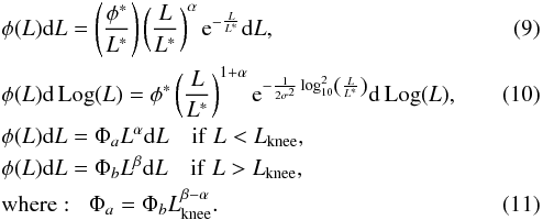 The double power law provides the worst fits in all cases and will not be considered in the further analysis. Indeed we do not observe a clear “knee” in the IR LF in groups (see Fig. 4) as observed instead in the total IR LF (e.g. Sanders et al. 2003; Magnelli et al. 2009, 2011, 2013). The group galaxy IR LF shows a smoother decline at high luminosity which is more consistent with a Schechter or a modified Schechter function than with a double power law. The double power law predicts too many bright galaxies at the bright end, especially in the two lowest redshift bins, where we observe a rather fast decline of the LF at very high luminosity. The Schecter and modified Schechter fits (both shown in Fig. 4) are of similar quality. Free parameters of the fits are the LF normalization and its “characteristic” or “knee” luminosity L∗. The LF slope parameter α is a free parameter only in the lowest redshift bin (0.1 <z< 0.4), where we sample the IR LF to relatively low values of LIR. We use this best-fit value of α for the higher redshift IR LFs, where the faint end is not well sampled by our data. A similar approach has been taken by Magnelli et al. (2009) and Gruppioni et al. (2013). At z< 0.1 for the IR LF derived from Guo et al. (2014), the shallower depth of the H-ATLAS survey does not allow constraining the LF faint end. Thus, in this case we fix α to the value estimated at 0.1 <z< 0.4. In the case of the modified Schechter function of Saunders et al. (1990), we fix the σ parameter to the value of 0.5 as in Gruppioni et al. (2013). The best-fit parameters are listed in Table 2.
Best-fit parameters of the IR LFs.
Consistently with the behaviour already observed in the total IR LF at similar redshifts (e.g. Magnelli et al. 2009, 2011, 2013; Gruppioni et al. 2013), the knee luminosity and the normalization of the group galaxy LF increases with redshift; that is, both the number of star forming galaxies in groups and their mean IR luminosity increase with redshift. This reflects the generally increasing SF activity of the Universe with redshift.
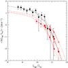 |
Fig. 5 Comparison of the IR LFs in groups (black filled points and solid lines) at 0.1 <z< 0.4 derived in this work and the group LFs of Guo et al. (2014) (red symbols and dashed lines) converted into IR LF derived at 0.1 < 0 < 0.2 (triangles), 0.2 < 0 < 0.3 (squares), and 0.3 <z< 0.4 (stars). For clarity we show here only the best fit derived with the modified Schechter function of Saunders et al. (1990). |
The comparison of our LFs with those derived by Guo et al. (2014) is shown in Fig. 5. Our determination of the group LFs reaches fainter luminosities, so we can only compare the bright end of the group LFs. While there is agreement between the Guo et al. and our LFs at the very bright end, though our error bar are very large, the normalizations are different, and the Guo et al. (2014) groups contain, on average, a lower number of IR-emitting galaxies than the groups observed in this work. It is hard to tell whether this is an effect of the blending problems of the very large SPIRE PSF of the H-ATLAS maps or of the different group-selection technique of Robotham et al. (2011). In the former case, the large SPIRE PSF at 250 μ of ~18 arcsec could lead to blending problems in crowded regions, such as groups and clusters. Two or a few relatively faint sources that are closer than the PSF are therefore identified as a single brighter source. This would subtract sources from the faint end towards the bright end. In the latter case, instead, the optical selection could lead to selecting low-richness groups for a given halo mass that are usually undetected in the X-rays. This would lead to a lower mean group richness, hence to a lower LF normalization.
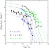 |
Fig. 6 Comparison of the IR LFs in groups (filled points) with the IR LF in clusters (stars). The colour code is the same as in Fig. 4: blue for the nearby groups of Guo et al. (2014) and the Shapley superclusters (Haines et al. 2010) at z< 0.1, black for 0.1 <z< 0.4 groups and 0.15 <z< 0.3 LoCuSS clusters (Haines et al. 2013), and green for 0.4 <z< 0.8 groups and for the 0.6 <z< 0.8 rich cluster LF of Finn et al. (2010). For clarity we only show here the best fit derived with the modified Schechter function of Saunders et al. (1990). |
For completeness we also compare the IR LFs in clusters available in the literature. Figure 6 shows the comparison of the Guo et al. (2014) IR LF in groups at z< 0.1 with the IR LF of the Shapley supercluster studied in Haines et al. (2010), which as shown in Haines et al. (2013), is consistent with the IR LF of the Coma cluster and A3266 studied by Bai et al. (2006) and Bai et al. (2009), respectively. Our IR LF in groups at 0.1 <z< 0.4 is compared with the stacked IR LF of 30 clusters observed at 0.15 <z< 0.30 in the LoCuSS survey (Haines et al. 2013). Our IR LF in groups at 0.4 <z< 0.8 is compared with the stacked IR LF of six rich clusters at 0.6 <z< 0.8 studied in Finn et al. (2010). We fit the cluster LFs with the Schechter and modified Schechter functions (see Table 2). The main difference between the group and the cluster LF is obviously the normalization, since the clusters are much richer, so they contain many more star-forming and IR-emitting galaxies. However, modulo the different normalization, the knee luminosity of cluster and group LFs shows a similar evolution (see also Fig. 8, upper panel).
 |
Fig. 7 Comparison of IR LF in groups (filled points) and the total IR LF (shaded red regions). The observed IR luminosity function in galaxy groups is indicated by the points with error bars. In the first redshift bin at z< 0.1, we show the IR LF in groups derived from Guo et al. (2014) and the best fit of the field IR LF of Sanders et al. (2003). At higher redshift we use the total IR LF of Gruppioni et al. (2013, red shaded region) and Magnelli et al. (2013, blue dashed line). The IR LF in groups modified Schechter function best fit is shown by the solid line in all cases. The different luminosity limit of the group LF with respect to the total LF of Gruppioni et al. (2013) and Magnelli et al. (2013) is because the group LF is also based on MIPS 24 μm data, while the general LF is based only on PACS data. |
4. Comparison with the total IR LF
In this section we compare the IR LF of our groups with the total IR LF at similar redshifts. For this we must first evaluate the IR LF of the group galaxies per unit of comoving volume. To do so, we multiply our determination of the group IR LF by the comoving number density of the dark matter haloes in the same mass range as a function of redshift (ρNhalo(z)). (We consider here the 1013 − 14 M⊙ halo mass range as the average normalization of the group IR LF is dominated by groups in this mass range.) We estimate ρNhalo(z) by using the WMAP9 concordance-model (Hinshaw et al. 2013) prediction of the comoving dN/dz of haloes in the mass range of our group sample. This model reproduces the observed log (N) − log (S) distribution of the deepest X-ray group and cluster surveys (see e.g. Finoguenov et al. 2010). For comparison we estimate the comoving dN/dz in the same mass bin, also according to the Planck cosmology based on the SZ Planck number counts (Planck Collaboration XX 2014). In this cosmology, the number of groups is 0.14 dex higher, on average, up to z ~ 1.5. We caution that the estimate of the IR LF of the group galaxy population at z ~ 1.6 is only tentative since it is based on one group only, which is relatively massive and might not be representative of the general group galaxy population at that redshift.
In Fig. 7 we show the IR LF of the group galaxy population, expressed as number of galaxies per unit of comoving volume, together with the total IR LFs as derived by Gruppioni et al. (2013) and Magnelli et al. (2013). The best-fit faint-end slope we determined for the 0.1 <z< 0.4 group LF is in remarkable agreement with the one obtained for the field LF by Gruppioni er al. (2013), while the LF of Magnelli et al. (2013) shows a steeper faint end, which is, however, consistent with the results of Magnelli et al. (2009, 2011) based on deeper Spitzer data. The shape of the IR LF in groups at 0.4 <z< 0.8 is consistent, in terms of L∗ and faint-end slope, with that of the total IR LF in the same redshift bin, even if the volume density of IR-emitting group galaxies is ~60% lower than the volume density of the total population. Indeed, if we re-normalize the group and the total IR LF to their integral over the same luminosity region, the two LFs overlap perfectly. This similarity is not observed in other redshift bins.
At z< 0.4, the group IR LF is characterized by a much steeper cut-off at the bright end than the total IR LF. Groups at this redshift lack the brightest, rarest, most star-forming IR galaxies that are instead observed in the field. In addition, the volume density of the group IR-emitting galaxies is much lower (less than 10%) than the volume density of the whole IR galaxy population.
At z ~ 1 the IR LF in groups and in the Kurk et al. (2008) structure exhibit a slighty brighter knee luminosity than the total LF (see also the upper panel of Fig. 8). In addition, the normalization of the LF indicates that the density of IR-emitting group galaxies is very close to the density of the total galaxy population. This indicates that at high redshift, the group galaxy population makes a substantial contribution to the IR emitting galaxy population as a whole. The slightly higher L∗ of the group galaxy LF indicates a potentially higher mean SFR in groups than in the field, at least in the star-forming galaxy population. This would be consistent with a flattening of the SFR-density relation at this redshift, as found by Ziparo et al. (2014), but also with a potential reversal of the same relation, though the difference between the total and group galaxy luminosity distribution is not very significant (~2σ, see Fig. 8).
For a more quantitative comparison, we show the best-fit values of the L∗ (upper panel) and Φ ∗ (lower panel) parameters of the modified Schechter function in Fig. 8, as a function of redshift, for both the group and the total IR LFs, and for the IR LF in clusters at the redshifts where these parameters have been estimated. To obtain the Φ ∗ of the cluster IR LF, we multiplied the cluster IR LF shown in Fig. 6 by the number density of cluster size haloes (at masses over 1014 M⊙) as a function of redshift. We only consider the IR LF of Gruppioni et al. (2013) here. A direct comparison with the LF of Magnelli et al. (2013) is not possible, since they use a double power law function that does not provide a good fit to the group LF.
The evolution of the knee luminosity seems to be faster in groups than for the total galaxy population. An power law does not provide a good fit to the L∗-redshift relation as in Gruppioni et al. (2013) and Magnelli et al. (2013). Most of the evolution seems to take place at z> 0.4. Below this redshift, both L∗ and Φ∗ are not evolving significantly. We observe a mild Φ∗ evolution as a function of redshift which is well fitted by a power law Φ∗ ∝ z-1.6.
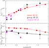 |
Fig. 8 Evolution of the best-fit L∗ (upper panel) and Φ∗ (bottom panel) parameters of the modified Schechter of Saunders et al. (1990) for the IR LF in groups (black points), the total IR LF of Gruppioni et al. (2013, red points), and the cluster IR LF (magenta points). Error bars are 1σ (when not shown they are smaller than the symbol size). |
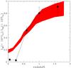 |
Fig. 9 Evolution of the fraction of IR luminosity due to the LIRGs in groups (black points) and in the total IR galaxy population (red shaded region). This is obtained as the ratio between the integral of the observed IR LF down to LIR> 1011 L⊙ and the integral estimated down to LIR> 107 L⊙ of the group and total IR LF, respectively. The red shaded region is obtained by considering in any redshift bin the whole range of possible values, including errors, derived from the total IR LF estimated by Sanders et al. (2003), Le Floc’h et al. (2005), Rodighiero et al. (2010), Magnelli et al. (2009, 2011, 2013), Gruppioni et al. (2013). |
To provide a more model-independent comparison, we show in Fig. 9 the fraction of IR luminosity due to LIRGs in groups and in the total IR galaxy population. This fraction is obtained as the ratio between the integral of the observed IR LF down to LIR> 1011 L⊙ and the integral estimated down to LIR> 107 L⊙ of the group and total IR LF, respectively. The two integrals are estimated by using both the observed LF in the luminosity range sampled by the observations and the best-fit LF (modified Schechter function) at fainter luminosities. Up to z = 1.2 the integral down to LIR = 1011 L⊙ is based entirely on the observed LF. The correction of the integral down to LIR = 107 L⊙ due to the extrapolation from the best fit LF is <10%. At z> 1 also the integral down to LIR = 1011 L⊙ must be corrected with an extrapolation of the best fit LFs. The correction is however very small (7% at the limit LIR = 1011 L⊙, and 15% down to LIR = 107 L⊙) because LIRGs account for most of the IR luminosity.
The contribution of the LIRG population in the total galaxy population is shown by the red region of Fig. 8. This region is obtained by considering in any redshift bin the whole range of possible values, including errors, derived from the total IR LF estimated by Sanders et al. (2003); Le Floc’h et al. (2005); Rodighiero et al. (2010); Magnelli et al. (2009, 2011, 2013); Gruppioni et al. (2013). We observe a significantly faster decline of the LIRG luminosity contribution in groups with respect to the total galaxy population. At high redshift (z> 0.4), the fractional luminosity contribution of LIRGs is similar in groups and in the total galaxy population. At lower redshift this contribution is close to zero in galaxy groups, while it is 5–10% in the total population.
There have been numerous studies on the origin and evolution of LIRGs, suggesting that these galaxies – at least in the local Universe – are triggered by strong interactions and mergers of gas-rich galaxies (see the review by Sanders & Mirabel 1996). The fraction of mergers among LIRGs increases with IR luminosity and approaches 100% for samples of nearby ULIRGs (Sanders et al. 1988; Kim et al. 1995; Clements et al. 1996; Farrah et al. 2001; Veilleux et al. 2002). At higher redshift, most of the LIRGs are MS galaxies, and they are generally not associated to merger activity (Bell et al. 2005; Elbaz et al. 2007, 2011). Thus, our findings seem to suggest that galaxy groups are not favorite sites for the onset of a strong merger activity, at least not among gas-rich galaxies and not at z< 1.
5. The contribution of group galaxies to the SFR density of the Universe
By integrating the group galaxy IR LFs, we derive the evolution of the comoving number density (Fig. 10) of “faint” galaxies (i.e., 107 L⊙<LIR< 1011 L⊙), LIRGs (i.e., 1011 L⊙<LIR< 1012 L⊙), and ULIRGs (i.e., LIR> 1012 L⊙), as done in Magnelli et al. (2013) for the total galaxy population. We point out that in the case of the “faint” galaxy population, the comoving densities mainly rely on the extrapolation of the LF, in particular at z> 0.4. Thus, we recommend caution when interpreting values not directly constrained by the Spitzer and Herschel observations. As already pointed out in Magnelli et al. (2013), we emphasize that the LIRG and ULIRG designations are used here strictly to segregate the luminosity bins, but not to imply physical properties. Indeed, Herschel studies have unambiguously revealed that high-redshift (U)LIRGs do not have the same properties as their local counterparts (e.g. Elbaz et al. 2011; Wuyts et al. 2011).
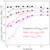 |
Fig. 10 Evolution of the comoving number density of faint IR emitting galaxies (107<LIR/L⊙< 1011, black symbols), LIRGs (1011 ≤ LIR/L⊙< 1012, red symbols), and ULIRGs (LIR/L⊙ ≥ 1012, magenta symbols) of the whole galaxy population (filled points) and of the group galaxy population (stars). The comoving number density of the total population is taken from Magnelli et al. (2013) at z> 0.1 and from Sanders et al. (2003) at z ~ 0. The dashed lines show the best fit relation between comoving number density and redshift, (1 + z)α (best-fit values of α are given in the text). |
We find that the number density of ULIRGs and LIRGs evolves strongly from redshift ~1, and the evolution is faster for groups than for the total galaxy population. The number density evolution is faster for IR-brighter galaxies, both in the field and in groups. We fit the number density vs. redshift of any given subsample with a power law of the type numberdensity ∝ (1 + z)α, up to z ~ 1. Beyond z ~ 1, the number densities of the different IR galaxy populations do not evolve any further. We find α = 0.73 ± 0.08,5.4 ± 0.5, and 8.9 ± 0.7 for the faint IR galaxies, LIRGs, and ULIRGs, respectively, in the field, and α = 4 ± 1,12 ± 2,22 ± 4 for the faint IR galaxies, LIRGs, and ULIRGs, respectively, in groups. The best-fit α values are significantly higher for group galaxies than for the total galaxy population, confirming the much faster decline of the number density of IR emitting galaxies in groups relative to the total population. The comoving number densities of faint IR galaxies, LIRGs, and ULIRGs decrease by factors ~1.5, 34 and 215, respectively, since z ~ 1, in the field, and by a factor 54, and 3.5 and 6 orders of magnitudes, respectively, in groups.
At z ~ 1, group galaxies contribute 40% to 60% of the whole IR galaxy population in the sub-ULIRG regime, but almost all ULIRGs are in groups. This is consistent with a reversal (Elbaz et al. 2007) or a flattening (Ziparo et al. 2014) of the SFR-density relation. In addition, there is also consistency with our previous findings that the fraction of bright IR galaxies (LIR> 1011 L⊙) is higher in a denser environment at z ~ 1 (Popesso et al. 2011). That ULIRGs are primarily located in massive haloes at high redshift is also consistent with the recent findings of Magliocchetti et al. (2013, 2014), who find that the clustering lengths of star-forming systems present a sharp increase as a function of redshift. This behaviour is reflected in the trend of the masses of the dark matter hosts of star-forming galaxies, which increase from 1011−11.5 M⊙ at z< 1 to ~1013.5 M⊙ between z ~ 1 and z ~ 2. Our analysis shows that galaxies which actively form stars at high redshifts are not the same population of sources we observe in the more local Universe. In fact, vigorous star formation in the early Universe is hosted by very massive structures, while for z< 1 a comparable activity is found in much smaller systems, consistent with the downsizing scenario.
By integrating our group galaxy IR LFs, we derive the evolution of the comoving IR luminosity density. We use the relation of Kennicutt (1998) to convert LIR into SFR and derive the contribution of the group galaxy population to the cosmic SFR density of the Universe in redshit bins. We assume that the IR flux is completely dominated by obscured SF rather than by AGN activity, also for the 5% of group members identified as X-ray-emitting AGNs. The hosts of 87% of these AGNs have been detected by PACS, and it has been shown that their IR emission originates in the host galaxy in >94% of the cases, that is it has a SF origin (Shao et al. 2010; Mullaney et al. 2012; Rosario et al. 2012). For the remaining 13% of AGNs, the 24 μm flux detected with Spitzer could in principle be contaminated by the AGN emission. However, since these galaxies are faint IR sources, and they represent only 0.65% of the entire group galaxy population studied in this work, their contribution is too marginal to have any significant effect on our estimates of the SFR density contributed by groups.
To properly derive the total SFR density of the Universe, Magnelli et al. (2013) combine the obscured SFR density with the unobscured SFR density of the Universe derived by Cucciati et al. (2012) using rest-frame UV observations. We do not have an estimate of the unobscured SFR density for the population of group galaxies. Thus, for a fair comparison, we consider the contribution of the group galaxy population only to the obscured cosmic SFR density. This does, however constitute most (75–88%) of the full cosmic SFR density at any redshift (Magnelli et al. 2013).
In Fig. 11 we show the contribution of the group galaxy population to the obscured cosmic SFR density. For completeness we also show the compilation of the SFR density estimates of Beacom & Hopkins (2006), which are based on both IR and UV data. At z ≳ 1 the group galaxy population makes a substantial (60–80%) contribution to the cosmic SFR density, because most of the z> 1 cosmic SFR density is provided by (U)LIRGs (Magnelli et al. 2009, 2011, 2013; Gruppioni et al. 2010, 2013), and a substantial fraction (70%) of LIRGs and the totality of ULIRGS of z> 1 are located in groups (see Fig. 10). At z ≲ 1 the rapid decline in the number density of (U)LIRGs in groups drives the similarly rapid decline in the group SFR density. While the cosmic SFR density declines by ~0.65 dex since z = 1, the contribution of group galaxies to the cosmic SFR density decreases by 1.43 dex, and becomes negligible by z ~ 0.
6. Discussion
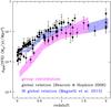 |
Fig. 11 Contribution of the group galaxy population (magenta shaded region) to the cosmic SFR density estimated by Magnelli et al. (2013, blue shaded region, obscured SFR density) and Beacom & Hopkins (2006, black points, total SFR density). |
At z< 0.4, the group IR LF is characterized by a much steeper cut-off at the bright end than the total IR LF. In other words, the very bright, rare, and strongly star-forming IR-emitting galaxies that are observed in the field do not reside in groups at z< 0.4. The volume density of group IR emitting galaxies is ≤10% that of the total population. At 0.4 <z< 0.8, we find consistency between the shapes (characterized by L∗ and faint end slope) of the group IR LF and the total IR LF, and the volume density of group IR emitting galaxies is only ~60% lower than for the total population. At z ~ 1 the galaxy group IR LF and the Kurk et al. (2008) structure LF exhibit a slighty brighter L∗ luminosity than the total LFs of Gruppioni et al. (2013), and Magnelli et al. (2013), respectively. This suggests that star-forming group galaxies have a slightly higher mean SFR than star-forming galaxies in the field. The volume density of IR-emitting group galaxies is very close to that of the total galaxy population; that is to say, the group galaxy population provides a ~70% of the LIRGs and the totality of the ULIRGS of the total IR-emitting galaxy population.
The comoving number density of (U)LIRGs in groups evolves strongly, since redshift ~1, and this evolution is much faster than observed for the total population of (U)LIRGs. The evolution is faster for IR-brighter galaxies, both in groups and in the field. Group LIRGs and other, less bright, group IR-emitting galaxies account for 40% to 60% of the whole IR galaxy population at z ~ 1, but almost all ULIRGs at the same redshift are located in groups. This is consistent with our previous result of a higher fraction of LIRGs in denser environments at z ~ 1 (Popesso et al. 2011). This is further evidence that the mean SFR in groups is higher than in the field at z ~ 1, consistent with previous findings that have suggested a reversal (Elbaz et al. 2007) or flattening (Ziparo et al. 2014) of the SFR-density relation. In addition, since most of high-redshift LIRGs are MS galaxies and are generally not associated to merger activity, our findings would suggest that galaxy groups are not favorite sites for the onset of a strong merger activity, at least not among gas-rich galaxies, and not at z< 1.
We show that at z ≳ 1 group galaxies contribute 60% to 80% to the cosmic SFR density, because (U)LIRGs are the main contributors to the cosmic SFR density at z> 1 (Magnelli et al. 2013; Gruppioni et al. 2013), and according to our results, they are largely group galaxies at that epoch. At z ≲ 1 the number density of (U)LIRGs in groups declines very rapidly, and this then leads to a similarly rapid decline in the contribution of group galaxies to the cosmic SFR density. By z ~ 0 this contribution becomes entirely negligible.
Our results agree with previous claims about a reversal or a flattening of the SFR-density relation (Elbaz et al. 2007; Popesso et al. 2011; Ziparo et al. 2013) at z ~ 1. Based on the same data set as used in this paper, Ziparo et al. (2013) conclude that the differential evolution of groups galaxies with respect to field galaxies is due to a faster quenching of main-sequence star-forming galaxies in groups than in the field. (High-z (U)LIRGs are main-sequence galaxies.)
These and our results clearly indicate that the SF activity of galaxies evolves differently in different environments. This is also supported by independent, observational evidence; for example, the galaxy red sequence forms earlier in groups than in the field, especially at high stellar masses (Iovino et al. 2010; Kovač et al. 2010), and there is a transient population of “red spirals” in groups not observed in the field (Balogh et al. 2011; Wolf et al. 2009; Mei et al. 2012), which suggests morphological transformations are in place in groups at least after z ~ 1. Quenching of SF activity therefore occurs earlier in galaxies that are embedded in more massive haloes than on average. In this sense, as in Popesso et al. (2012), we see evidence of a “halo downsizing” effect, whereby massive haloes evolve more rapidly than haloes with lower masses (Neistein et al. 2006). This “halo downsizing” effect is not at odds with the current hierarchical paradigm of structure formation. It implies that the quenching process is driven by the accretion of galaxies from the cosmic web into more massive haloes. Halo downsizing then comes naturally in the hierarchical scenario. In fact, massive galaxies are hosted by massive haloes, and haloes in overdense regions on average form earlier and merge more rapidly than haloes in regions of average density (Gao et al. 2004).
To isolate the physical processes responsible for the quenching of SF activity, Peng et al. (2010) have identified two types of quenching, one dependent on the galaxy “mass” and another dependent on the galaxy “environment”. The AGN feedback can be ascribed to the “mass” quenching type. Powerful jets (radio mode) or outflows (quasar mode) driven by the AGN activity swipe out the gas from the AGN host galaxy, at the same time halting gas accretion onto the central black hole and the SF activity of the host galaxy. This process only depends on the individual galaxy properties, such as its stellar mass, which is proportional to the mass of the central black hole. This process cannot be responsible for the “halo downsizing” we observe. The faster evolution of the group galaxy population is observed for galaxies of any IR luminosity, hence, of any stellar mass, given the relation known as the main sequence of SF galaxies (Noeske et al. 2007; Elbaz et al. 2007), which is also obeyed (at high-z) by (U)LIRGs. If AGN feedback is only dependent on galaxy mass, the evolution should be similar among (U)LIRGs in the field and in groups, but it is not.
We therefore need to appeal to “environment” quenching to explain our results. Related to the “environment” quenching are the processes identified by the cold-hot two-mode gas accretion model (Kereš et al. 2005; Dekel & Birnboim 2006). According to this model, large haloes primarily accrete hot gas while small haloes primarily accrete cold gas. In the cold accretion paradigm, the gas cooling along filaments tends to fall to the centre of the halo, so that galaxies that turn into satellites become disconnected from their feeding filaments.
In semi-analytical models, such as those based on the Millennium Simulation (Springel et al. 2005), this physical process is implemented by a sudden cut-off of the cold gas supply as a galaxy enters massive haloes dominated by hot accretion. This leads to an immediate quenching of gas accretion, and, consequently, of SF activity. This implementation of the “environment” quenching leads to a rapid evolution of the galaxy population of massive haloes, which turn into a 90% red and dead galaxy population already by redshift ~2. As a consequence, there is an excess of red and passive galaxies in groups and clusters in the simulated local Universe with respect to the observations (Wang et al. 2007), the so-called “satellite over-quenching” problem. Therefore, in these models, galaxies in haloes with mass higher than 1012 M⊙ provide a very marginal contribution to the CSFR density at any redshift (van de Voort et al. 2011), and this is clearly at odds with our results.
Recently, using SPH simulations, Simha et al. (2009) have shown that satellite galaxies continue to accrete gas and convert it into stars for quite some time (0.5–1 Gyr) after entering a larger halo, where gas is hot. The gas accretion declines steadily over this period, leading to gradual quenching. Observational support for a longer quenching timescale than predicted by traditional semi-analytical models has recently come from the analysis Wetzel et al. (2013). They do not suggest a gradual quenching, but a rapid one (<0.8 Gyr), which however occurs only 2–4 Gyr after the satellite infall into groups/clusters. As argued by Simha et al. (2009), allowing for a longer quenching timescale after satellite accretion should improve the agreement of semi-analytic models with the observed colour distributions of satellite galaxies in groups and with the observed colour dependence of galaxy clustering. Better agreement with the observed evolution of the SF activity in groups is also to be expected.
7. Summary and conclusions
We have determined the IR LF of group galaxies in the redshift range z = 0–1.6, based on a sample of 39 X-ray selected groups with extensive spectroscopic and photometric data available, in particular, from Spitzer MIPS and Herschel PACS.
We find a differential evolution of the IR LFs of group and field galaxies. The group IR LF at low-z lacks very IR-bright galaxies in the field, and group IR-emitting galaxies contribute ≲10% of the comoving volume density of the IR galaxy population as a whole. The fraction of very IR-bright galaxies (LIRGs and ULIRGs) increases rapidly with z, and this increase is much faster in groups than in the general population. As a result, the shape of the group galaxy IR LF first becomes similar to that of field galaxies (at intermediate redshifts, 0.4 < z < 0.8) and then, at z ~ 1, it shows an excess of very IR-bright galaxies with respect to the field IR LF. The contribution of group IR-emitting galaxies to the comoving volume density of the IR galaxy population as a whole also increases with redshift, reaching ~40% at z ~ 0.5 and ~60–70% at z ~ 1.
We quantify this differential evolution of the group and field IR LFs also in terms of the comoving number density of (U)LIRGs in groups and in the general population. We find that almost all ULIRGs are located in groups at z ~ 1, while they are almost all outside groups at z ~ 0. Finally, we quantify the contribution of group galaxies to the cosmic SFR density, and find it to increasing from virtually none at z ~ 0 to 60–80% at z ~ 1.
Our results indicate “halo downsizing” in the star formation processes of galaxies. Since the differential evolution we observe not only concerns very bright (hence massive) galaxies (i.e. LIRGs and ULIRGs) but also IR-emitting galaxies of lower luminosities, we argue that “mass” quenching alone cannot explain our results, so “environment” quenching is also required.
The mass M200 is the mass enclosed within a sphere of radius r200, where r200 is the radius where the mean mass overdensity of the group is 200 times the critical density of the Universe at the group mean redshift.
Acknowledgments
The authors aknowledge G. Zamorani for the very useful comments on the early draft. PACS has been developed by a consortium of institutes led by MPE (Germany) and including UVIE (Austria); KUL, CSL, IMEC (Belgium); CEA, OAMP (France); MPIA (Germany); IFSI, OAP/AOT, OAA/CAISMI, LENS, SISSA (Italy); IAC (Spain). This development has been supported by the funding agencies BMVIT (Austria), ESA-PRODEX (Belgium), CEA/CNES (France), DLR (Germany), ASI (Italy), and CICYT/MCYT (Spain). We gratefully acknowledge the contributions of the entire COSMOS collaboration consisting of more than 100 scientists. More information about the COSMOS survey is available at http://www.astro.caltech.edu/~cosmos. This research made use of NASA’s Astrophysics Data System, of NED, which is operated by JPL/Caltech, under contract with NASA, and of SDSS, which has been funded by the Sloan Foundation, NSF, the US Department of Energy, NASA, the Japanese Monbukagakusho, the Max Planck Society, and the Higher Education Funding Council of England. The SDSS is managed by the participating institutions (http://www.sdss.org/collaboration/credits.html).
References
- Bai, L., Rieke, G. H., Rieke, M. J., et al. 2006, ApJ, 639, 827 [NASA ADS] [CrossRef] [Google Scholar]
- Bai, L., Rieke, G. H., Rieke, M. J., Christlein, D., & Zabludoff, A. I. 2009, ApJ, 693, 1840 [NASA ADS] [CrossRef] [Google Scholar]
- Balestra, I., Mainieri, V., Popesso, P., et al. 2010, A&A, 512, A12 [NASA ADS] [CrossRef] [EDP Sciences] [Google Scholar]
- Balogh, M. L., McGee, S. L., Wilman, D. J., et al. 2011, MNRAS, 412, 2303 [Google Scholar]
- Barger, A. J., Cowie, L. L., & Wang, W.-H. 2008, ApJ, 689, 687 [NASA ADS] [CrossRef] [Google Scholar]
- Bell, E. F. 2003, ApJ, 586, 794 [Google Scholar]
- Bell, E. F., Papovich, C., Wolf, C., et al. 2005, ApJ, 625, 23 [NASA ADS] [CrossRef] [Google Scholar]
- Berta, S., Magnelli, B., Lutz, D., et al. 2010, A&A, 518, L30 [NASA ADS] [CrossRef] [EDP Sciences] [Google Scholar]
- Biviano, A., Fadda, D., Durret, F., Edwards, L. O. V., & Marleau, F. 2011, A&A, 532, A77 [NASA ADS] [CrossRef] [EDP Sciences] [Google Scholar]
- Buat, V., Boselli, A., Gavazzi, G., & Bonfanti, C. 2002, A&A, 383, 801 [NASA ADS] [CrossRef] [EDP Sciences] [Google Scholar]
- Capak, P., Aussel, H., Ajiki, M., et al. 2007, ApJS, 172, 99 [NASA ADS] [CrossRef] [Google Scholar]
- Caputi, K. I., Lagache, G., Yan, L., et al. 2007, ApJ, 660, 97 [NASA ADS] [CrossRef] [Google Scholar]
- Cardamone, C. N., van Dokkum, P. G., Urry, C. M., et al. 2010, ApJS, 189, 270 [NASA ADS] [CrossRef] [Google Scholar]
- Chung, S. M., Gonzalez, A. H., Clowe, D., Markevitch, M., & Zaritsky, D. 2010, ApJ, 725, 1536 [NASA ADS] [CrossRef] [Google Scholar]
- Cimatti, A., Robberto, M., Baugh, C., et al. 2008, Exp. Astron., 37 [Google Scholar]
- Clements, D. L., Sutherland, W. J., McMahon, R. G., & Saunders, W. 1996, MNRAS, 279, 477 [NASA ADS] [CrossRef] [Google Scholar]
- Colless, M. 1989, MNRAS, 237, 799 [NASA ADS] [CrossRef] [Google Scholar]
- Cooper, M. C., Newman, J. A., Weiner, B. J., et al. 2008, MNRAS, 383, 1058 [Google Scholar]
- Cooper, M. C., Yan, R., Dickinson, M., et al. 2012, MNRAS, 425, 2116 [NASA ADS] [CrossRef] [Google Scholar]
- Cowie, L. L., Barger, A. J., Fomalont, E. B., & Capak, P. 2004, ApJ, 603, L69 [NASA ADS] [CrossRef] [Google Scholar]
- Cucciati, O., Tresse, L., Ilbert, O., et al. 2012, A&A, 539, A31 [NASA ADS] [CrossRef] [EDP Sciences] [Google Scholar]
- De Propris, R., Colless, M., Driver, S. P., et al. 2003, MNRAS, 342, 725 [NASA ADS] [CrossRef] [Google Scholar]
- Dekel, A., & Birnboim, Y. 2006, MNRAS, 368, 2 [NASA ADS] [CrossRef] [Google Scholar]
- Dressler, A. 1980, ApJ, 236, 351 [NASA ADS] [CrossRef] [Google Scholar]
- Eke, V. R., Baugh, C. M., Cole, S., et al. 2005, MNRAS, 362, 1233 [NASA ADS] [CrossRef] [Google Scholar]
- Elbaz, D., Daddi, E., Le Borgne, D., et al. 2007, A&A, 468, 33 [NASA ADS] [CrossRef] [EDP Sciences] [Google Scholar]
- Elbaz, D., Dickinson, M., Hwang, H. S., et al. 2011, A&A, 533, A119 [NASA ADS] [CrossRef] [EDP Sciences] [Google Scholar]
- Farrah, D., Rowan-Robinson, M., Oliver, S., et al. 2001, MNRAS, 326, 1333 [NASA ADS] [CrossRef] [Google Scholar]
- Feruglio, C., Aussel, H., Le Floc’h, E., et al. 2010, ApJ, 721, 607 [NASA ADS] [CrossRef] [Google Scholar]
- Finn, R. A., Desai, V., Rudnick, G., et al. 2010, ApJ, 720, 87 [Google Scholar]
- Finoguenov, A., Connelly, J. L., Parker, L. C., et al. 2009, ApJ, 704, 564 [NASA ADS] [CrossRef] [Google Scholar]
- Finoguenov, A., Watson, M. G., Tanaka, M., et al. 2010, MNRAS, 403, 2063 [NASA ADS] [CrossRef] [Google Scholar]
- Gao, L., De Lucia, G., White, S. D. M., & Jenkins, A. 2004, MNRAS, 352, L1 [NASA ADS] [CrossRef] [Google Scholar]
- Gómez, P. L., Nichol, R. C., Miller, C. J., et al. 2003, ApJ, 584, 210 [NASA ADS] [CrossRef] [Google Scholar]
- Gruppioni, C., Pozzi, F., Zamorani, G., & Vignali, C. 2011, MNRAS, 416, 70 [NASA ADS] [CrossRef] [Google Scholar]
- Gruppioni, C., Pozzi, F., Rodighiero, G., et al. 2013, MNRAS, 432, 23 [NASA ADS] [CrossRef] [Google Scholar]
- Guo, Q., Lacey, C., Norberg, P., et al. 2014, MNRAS, 442, 2253 [NASA ADS] [CrossRef] [Google Scholar]
- Haines, C. P., Smith, G. P., Pereira, M. J., et al. 2010, A&A, 518, L19 [NASA ADS] [CrossRef] [EDP Sciences] [Google Scholar]
- Haines, C. P., Pereira, M. J., Smith, G. P., et al. 2013, ApJ, 775, 126 [NASA ADS] [CrossRef] [EDP Sciences] [Google Scholar]
- Heavens, A., Panter, B., Jimenez, R., & Dunlop, J. 2004, Nature, 428, 625 [NASA ADS] [CrossRef] [PubMed] [Google Scholar]
- Hinshaw, G., Larson, D., Komatsu, E., et al. 2013, ApJS, 208, 19 [NASA ADS] [CrossRef] [Google Scholar]
- Ilbert, O., Salvato, M., Le Floc’h, E., et al. 2010, ApJ, 709, 644 [NASA ADS] [CrossRef] [Google Scholar]
- Iovino, A., Cucciati, O., Scodeggio, M., et al. 2010, A&A, 509, A40 [NASA ADS] [CrossRef] [EDP Sciences] [Google Scholar]
- Kennicutt, Jr., R. C. 1998, ARA&A, 36, 189 [Google Scholar]
- Kereš, D., Katz, N., Weinberg, D. H., & Davé, R. 2005, MNRAS, 363, 2 [NASA ADS] [CrossRef] [Google Scholar]
- Kim, D.-C., Sanders, D. B., Veilleux, S., Mazzarella, J. M., & Soifer, B. T. 1995, ApJS, 98, 129 [NASA ADS] [CrossRef] [Google Scholar]
- Kovač, K., Lilly, S. J., Knobel, C., et al. 2010, ApJ, 718, 86 [NASA ADS] [CrossRef] [Google Scholar]
- Kurk, J., Cimatti, A., Zamorani, G., et al. 2008, in Panoramic Views of Galaxy Formation and Evolution, eds. T. Kodama, T. Yamada, & K. Aoki, ASP Conf. Ser., 399, 332 [Google Scholar]
- Le Floc’h, E., Papovich, C., Dole, H., et al. 2005, ApJ, 632, 169 [NASA ADS] [CrossRef] [Google Scholar]
- Le Floc’h, E., Aussel, H., Ilbert, O., et al. 2009, ApJ, 703, 222 [NASA ADS] [CrossRef] [Google Scholar]
- Leauthaud, A., Finoguenov, A., Kneib, J.-P., et al. 2010, ApJ, 709, 97 [NASA ADS] [CrossRef] [Google Scholar]
- Lilly, S. J., Le Fèvre, O., Renzini, A., et al. 2007, ApJS, 172, 70 [NASA ADS] [CrossRef] [Google Scholar]
- Lilly, S. J., Le Brun, V., Maier, C., et al. 2009, ApJS, 184, 218 [Google Scholar]
- Lutz, D., Poglitsch, A., Altieri, B., et al. 2011, A&A, 532, A90 [NASA ADS] [CrossRef] [EDP Sciences] [Google Scholar]
- Magliocchetti, M., Popesso, P., Rosario, D., et al. 2013, MNRAS, 433, 127 [NASA ADS] [CrossRef] [Google Scholar]
- Magliocchetti, M., Lapi, A., Negrello, M., De Zotti, G., & Danese, L. 2014, MNRAS, 437, 2263 [NASA ADS] [CrossRef] [Google Scholar]
- Magnelli, B., Elbaz, D., Chary, R. R., et al. 2009, A&A, 496, 57 [NASA ADS] [CrossRef] [EDP Sciences] [Google Scholar]
- Magnelli, B., Elbaz, D., Chary, R. R., et al. 2011, A&A, 528, A35 [Google Scholar]
- Magnelli, B., Popesso, P., Berta, S., et al. 2013, A&A, 553, A132 [NASA ADS] [CrossRef] [EDP Sciences] [Google Scholar]
- Mamon, G. A., Biviano, A., & Boué, G. 2013, MNRAS, 429, 3079 [NASA ADS] [CrossRef] [Google Scholar]
- Mei, S., Stanford, S. A., Holden, B. P., et al. 2012, ApJ, 754, 141 [Google Scholar]
- Mullaney, J. R., Pannella, M., Daddi, E., et al. 2012, MNRAS, 419, 95 [NASA ADS] [CrossRef] [Google Scholar]
- Neistein, E., van den Bosch, F. C., & Dekel, A. 2006, MNRAS, 372, 933 [NASA ADS] [CrossRef] [Google Scholar]
- Nordon, R., Lutz, D., Shao, L., et al. 2010, A&A, 518, L24 [NASA ADS] [CrossRef] [EDP Sciences] [Google Scholar]
- Papovich, C., Momcheva, I., Willmer, C. N. A., et al. 2010, ApJ, 716, 1503 [NASA ADS] [CrossRef] [Google Scholar]
- Pérez-González, P. G., Rieke, G. H., Egami, E., et al. 2005, ApJ, 630, 82 [NASA ADS] [CrossRef] [Google Scholar]
- Planck Collaboration XX. 2014, A&A, 571, A20 [NASA ADS] [CrossRef] [EDP Sciences] [Google Scholar]
- Popesso, P., Dickinson, M., Nonino, M., et al. 2009, A&A, 494, 443 [NASA ADS] [CrossRef] [EDP Sciences] [Google Scholar]
- Popesso, P., Rodighiero, G., Saintonge, A., et al. 2011, A&A, 532, A145 [NASA ADS] [CrossRef] [EDP Sciences] [Google Scholar]
- Popesso, P., Biviano, A., Rodighiero, G., et al. 2012, A&A, 537, A58 [NASA ADS] [CrossRef] [EDP Sciences] [Google Scholar]
- Prescott, M. K. M., Impey, C. D., Cool, R. J., & Scoville, N. Z. 2006, ApJ, 644, 100 [NASA ADS] [CrossRef] [Google Scholar]
- Reddy, N. A., Steidel, C. C., Pettini, M., et al. 2008, ApJS, 175, 48 [NASA ADS] [CrossRef] [Google Scholar]
- Rettura, A., Rosati, P., Nonino, M., et al. 2010, ApJ, 709, 512 [NASA ADS] [CrossRef] [Google Scholar]
- Robotham, A. S. G., Norberg, P., Driver, S. P., et al. 2011, MNRAS, 416, 2640 [NASA ADS] [CrossRef] [Google Scholar]
- Rodighiero, G., Vaccari, M., Franceschini, A., et al. 2010, A&A, 515, A8 [NASA ADS] [CrossRef] [EDP Sciences] [Google Scholar]
- Rosario, D. J., Santini, P., Lutz, D., et al. 2012, A&A, 545, A45 [NASA ADS] [CrossRef] [EDP Sciences] [Google Scholar]
- Rykoff, E. S., Koester, B. P., Rozo, E., et al. 2012, ApJ, 746, 178 [NASA ADS] [CrossRef] [Google Scholar]
- Sanders, D. B., & Mirabel, I. F. 1996, ARA&A, 34, 749 [NASA ADS] [CrossRef] [Google Scholar]
- Sanders, D. B., Soifer, B. T., Elias, J. H., et al. 1988, ApJ, 325, 74 [NASA ADS] [CrossRef] [Google Scholar]
- Sanders, D. B., Mazzarella, J. M., Kim, D.-C., Surace, J. A., & Soifer, B. T. 2003, AJ, 126, 1607 [Google Scholar]
- Sanders, D. B., Salvato, M., Aussel, H., et al. 2007, ApJS, 172, 86 [Google Scholar]
- Santini, P., Fontana, A., Grazian, A., et al. 2009, A&A, 504, 751 [NASA ADS] [CrossRef] [EDP Sciences] [Google Scholar]
- Santini, P., Rosario, D. J., Shao, L., et al. 2012, A&A, 540, A109 [NASA ADS] [CrossRef] [EDP Sciences] [Google Scholar]
- Saunders, W., Rowan-Robinson, M., Lawrence, A., et al. 1990, MNRAS, 242, 318 [NASA ADS] [CrossRef] [Google Scholar]
- Scoville, N., Capak, P., Giavalisco, M., et al. 2007, in The Science Opportunities of the Warm Spitzer Mission Workshop, eds. L. J. Storrie-Lombardi, & N. A. Silbermann, AIP Conf. Ser., 943, 221 [Google Scholar]
- Shao, L., Lutz, D., Nordon, R., et al. 2010, A&A, 518, L26 [NASA ADS] [CrossRef] [EDP Sciences] [Google Scholar]
- Silverman, J. D., Mainieri, V., Salvato, M., et al. 2010, ApJS, 191, 124 [NASA ADS] [CrossRef] [Google Scholar]
- Simha, V., Weinberg, D. H., Davé, R., et al. 2009, MNRAS, 399, 650 [NASA ADS] [CrossRef] [Google Scholar]
- Springel, V., White, S. D. M., Jenkins, A., et al. 2005, Nature, 435, 629 [NASA ADS] [CrossRef] [PubMed] [Google Scholar]
- Tanaka, M., Finoguenov, A., Mirkazemi, M., et al. 2013, PASJ, 65, 17 [NASA ADS] [Google Scholar]
- Tran, K.-V. H., Saintonge, A., Moustakas, J., et al. 2009, ApJ, 705, 809 [NASA ADS] [CrossRef] [Google Scholar]
- Trump, J. R., Impey, C. D., McCarthy, P. J., et al. 2007, ApJS, 172, 383 [NASA ADS] [CrossRef] [Google Scholar]
- van de Voort, F., Schaye, J., Booth, C. M., & Dalla Vecchia, C. 2011, MNRAS, 415, 2782 [Google Scholar]
- Vanzella, E., Cristiani, S., Dickinson, M., et al. 2006, A&A, 454, 423 [NASA ADS] [CrossRef] [EDP Sciences] [Google Scholar]
- Veilleux, S., Kim, D.-C., & Sanders, D. B. 2002, ApJS, 143, 315 [NASA ADS] [CrossRef] [Google Scholar]
- Wang, Y., Yang, X., Mo, H. J., & van den Bosch, F. C. 2007, ApJ, 664, 608 [NASA ADS] [CrossRef] [Google Scholar]
- Wetzel, A. R., Tinker, J. L., Conroy, C., & van den Bosch, F. C. 2013, MNRAS, 432, 336 [NASA ADS] [CrossRef] [Google Scholar]
- Wolf, C., Aragón-Salamanca, A., Balogh, M., et al. 2009, in The Starburst-AGN Connection, eds. W. Wang, Z. Yang, Z. Luo, & Z. Chen, ASP Conf. Ser., 408, 248 [Google Scholar]
- Wuyts, S., Förster Schreiber, N. M., Lutz, D., et al. 2011, ApJ, 738, 106 [NASA ADS] [CrossRef] [Google Scholar]
- Ziparo, F., Popesso, P., Biviano, A., et al. 2013, MNRAS, 434, 3089 [NASA ADS] [CrossRef] [Google Scholar]
- Ziparo, F., Popesso, P., Finoguenov, A., et al. 2014, MNRAS, 437, 458 [NASA ADS] [CrossRef] [Google Scholar]
All Tables
All Figures
|
Fig. 1 Mean spectroscopic completeness in the Spitzer MIPS 24 μm band across all the areas of the ECDFS, GOODS-N, and COSMOS field. |
| In the text | |
|
Fig. 2 Mean spectroscopic completeness in the Spitzer MIPS 24 μm band in the group regions as a function of the redshifts. The mean completeness is estimated for groups in different redshift bins and in different fields. The green sysmbols show the mean completeness for groups in ECDFS, magenta symbols show the mean completeness for groups in GOODS-N, and red symbols show the one for the COSMOS groups. They are grouped in three redshift bins: z< 0.4 (filled circles), 0.4 <z< 0.8 (filled triangles), and 0.8 <z< 1.2 (stars). The empy squares show the completeness in the region of the Kurk et al. (2008) structure at z ~ 1.6 in ECDFS. The mean completeness of the groups in each redshift bin is estimated in the group region within an annulus of 3 × r200 from the group centre. To guide the eye, the black dashed lines in the figure show the 24 μm flux corresponding to the LIRG limit (LIR = 1011 L⊙) at low (z ~ 0.1), intermediate (z ~ 0.5), and high (z ~ 1) redshift. The solid red line shows the 60 μJy limit used to estimate the mean group completeness. |
| In the text | |
|
Fig. 3 Group masses M200 vs. mean redshifts. |
| In the text | |
|
Fig. 4 IR LFs in galaxy groups estimated within 2 × r200 in different redshift bins: 0 <z< 0.4 (black points), 0.4 <z< 0.8 (green points), 0.8 <z< 1.2 (red points), and at z ~ 1.6 (magenta points; this is the IR LF of the structure of Kurk et al. 2008). Error bars are 1σ. The IR LF in groups in the lowest redshift bin at z< 0.1 (blue points) is obtained by averaging the IR LF in groups obtained in three different group halo mass bins by Guo et al. (2014). The solid (resp. dashed) lines, colour–coded as the points of the IR LF, indicate the best fit Schechter (resp. modified Schechter, see Saunders et al. 1990) functions. |
| In the text | |
|
Fig. 5 Comparison of the IR LFs in groups (black filled points and solid lines) at 0.1 <z< 0.4 derived in this work and the group LFs of Guo et al. (2014) (red symbols and dashed lines) converted into IR LF derived at 0.1 < 0 < 0.2 (triangles), 0.2 < 0 < 0.3 (squares), and 0.3 <z< 0.4 (stars). For clarity we show here only the best fit derived with the modified Schechter function of Saunders et al. (1990). |
| In the text | |
|
Fig. 6 Comparison of the IR LFs in groups (filled points) with the IR LF in clusters (stars). The colour code is the same as in Fig. 4: blue for the nearby groups of Guo et al. (2014) and the Shapley superclusters (Haines et al. 2010) at z< 0.1, black for 0.1 <z< 0.4 groups and 0.15 <z< 0.3 LoCuSS clusters (Haines et al. 2013), and green for 0.4 <z< 0.8 groups and for the 0.6 <z< 0.8 rich cluster LF of Finn et al. (2010). For clarity we only show here the best fit derived with the modified Schechter function of Saunders et al. (1990). |
| In the text | |
|
Fig. 7 Comparison of IR LF in groups (filled points) and the total IR LF (shaded red regions). The observed IR luminosity function in galaxy groups is indicated by the points with error bars. In the first redshift bin at z< 0.1, we show the IR LF in groups derived from Guo et al. (2014) and the best fit of the field IR LF of Sanders et al. (2003). At higher redshift we use the total IR LF of Gruppioni et al. (2013, red shaded region) and Magnelli et al. (2013, blue dashed line). The IR LF in groups modified Schechter function best fit is shown by the solid line in all cases. The different luminosity limit of the group LF with respect to the total LF of Gruppioni et al. (2013) and Magnelli et al. (2013) is because the group LF is also based on MIPS 24 μm data, while the general LF is based only on PACS data. |
| In the text | |
|
Fig. 8 Evolution of the best-fit L∗ (upper panel) and Φ∗ (bottom panel) parameters of the modified Schechter of Saunders et al. (1990) for the IR LF in groups (black points), the total IR LF of Gruppioni et al. (2013, red points), and the cluster IR LF (magenta points). Error bars are 1σ (when not shown they are smaller than the symbol size). |
| In the text | |
|
Fig. 9 Evolution of the fraction of IR luminosity due to the LIRGs in groups (black points) and in the total IR galaxy population (red shaded region). This is obtained as the ratio between the integral of the observed IR LF down to LIR> 1011 L⊙ and the integral estimated down to LIR> 107 L⊙ of the group and total IR LF, respectively. The red shaded region is obtained by considering in any redshift bin the whole range of possible values, including errors, derived from the total IR LF estimated by Sanders et al. (2003), Le Floc’h et al. (2005), Rodighiero et al. (2010), Magnelli et al. (2009, 2011, 2013), Gruppioni et al. (2013). |
| In the text | |
|
Fig. 10 Evolution of the comoving number density of faint IR emitting galaxies (107<LIR/L⊙< 1011, black symbols), LIRGs (1011 ≤ LIR/L⊙< 1012, red symbols), and ULIRGs (LIR/L⊙ ≥ 1012, magenta symbols) of the whole galaxy population (filled points) and of the group galaxy population (stars). The comoving number density of the total population is taken from Magnelli et al. (2013) at z> 0.1 and from Sanders et al. (2003) at z ~ 0. The dashed lines show the best fit relation between comoving number density and redshift, (1 + z)α (best-fit values of α are given in the text). |
| In the text | |
|
Fig. 11 Contribution of the group galaxy population (magenta shaded region) to the cosmic SFR density estimated by Magnelli et al. (2013, blue shaded region, obscured SFR density) and Beacom & Hopkins (2006, black points, total SFR density). |
| In the text | |
Current usage metrics show cumulative count of Article Views (full-text article views including HTML views, PDF and ePub downloads, according to the available data) and Abstracts Views on Vision4Press platform.
Data correspond to usage on the plateform after 2015. The current usage metrics is available 48-96 hours after online publication and is updated daily on week days.
Initial download of the metrics may take a while.