| Issue |
A&A
Volume 574, February 2015
|
|
|---|---|---|
| Article Number | A32 | |
| Number of page(s) | 15 | |
| Section | Extragalactic astronomy | |
| DOI | https://doi.org/10.1051/0004-6361/201423612 | |
| Published online | 20 January 2015 | |
Exceptional AGN-driven turbulence inhibits star formation in the 3C 326N radio galaxy⋆
1 Institut d’Astrophysique de Paris, CNRS, UMR 7095, 98 bis Boulevard Arago, 75014 Paris, France
e-mail: This email address is being protected from spambots. You need JavaScript enabled to view it.
2 Sorbonne Universités, UPMC Université Paris 06, 4 place Jussieu, 75005 Paris, France
3 Institut d’Astrophysique Spatiale, UMR 8617, CNRS, Université Paris-Sud, Bât. 121, 91405 Orsay, France
4 Spitzer Science Center, IPAC, California Institute of Technology, Pasadena, CA 92215, USA
5 Observatoire de Paris, LERMA, UMR 8112, CNRS, 61 avenue de l’Observatoire, 75014 Paris, France
6 LERMA/LRA, École Normale Supérieure and Observatoire de Paris, CNRS, 24, rue Lhomond, 75005 Paris, France
7 Department of Physical Sciences, The Open University, Milton Keynes MK7 6AA, UK
Received: 10 February 2014
Accepted: 10 October 2014
Abstract
We detect bright [Cii]λ158 μm line emission from the radio galaxy 3C 326N at z = 0.09, which shows no sign of ongoing or recent star formation (SFR< 0.07 M⊙ yr-1) despite having strong H2 line emission and a substantial amount of molecular gas (2 × 10⁹ M⊙, inferred from the modeling of the far-infrared (FIR) dust emission and the CO(1−0) line emission). The [Cii] line is twice as strong as the 0−0S(1) 17 μm H2 line, and both lines are much in excess of what is expected from UV heating. We combine infrared Spitzer and Herschel photometry and line spectroscopy with gas and dust modeling to infer the physical conditions in the [Cii]-emitting gas. The [Cii] line, like rotational H2 emission, traces a significant fraction (30 to 50%) of the total molecular gas mass. This gas is warm (70 <T< 100 K) and at moderate densities 700 <nH< 3000 cm-3, constrained by both the observed [Cii]-to-[Oi] and [Cii]-to-FIR ratios. The [Cii] line is broad, asymmetric, with a redshifted core component (FWHM = 390 km s-1) and a very broad blueshifted wing (FWHM = 810 km s-1). The line profile of [Cii] is similar to the profiles of the near-infrared H2 lines and the Na D optical absorption lines, and is likely to be shaped by a combination of rotation, outflowing gas, and turbulence. If the line wing is interpreted as an outflow, the mass loss rate would be higher than 20 M⊙ yr-1, and the depletion timescale close to the orbital timescale (≈ 3 × 10⁷ yr). If true, we are observing this object at a very specific and brief time in its evolution, assuming that the disk is not replenished. Although there is evidence of an outflow in this source, we caution that the outflow rates may be overestimated because the stochastic injection of turbulent energy on galactic scales can create short-lived, large velocity increments that contribute to the skewness of the line profile and mimic outflowing gas. The gas physical conditions raise the issue of the heating mechanism of the warm gas, and we show that the dissipation of turbulent energy is the main heating process. Cosmic rays can also contribute to the heating, but cannot be the dominant heating source because it requires an average gas density that is higher than the observational constraints. After subtracting the contribution of the disk rotation, we estimate the turbulent velocity dispersion of the molecular gas to be 120 <σturb< 330 km s-1, which corresponds to a turbulent heating rate that is higher than the gas cooling rate computed from the line emission. The dissipation timescale of the turbulent energy (2 × 10⁷ − 108 yrs) is comparable to or larger than the jet lifetime or the dynamical timescale of the outflow, which means that turbulence can be sustained during the quiescent phases when the radio jet is shut off. The strong turbulent support maintains a very high gas scale height (0.3 to 4 kpc) in the disk. The cascade of turbulent energy can inhibit the formation of gravitationally bound structures on all scales, which offers a natural explanation for the lack of ongoing star formation in 3C 326N, despite its having sufficient molecular gas to form stars at a rate of a few solar mass per year. To conclude, the bright [Cii] line indicates that strong AGN jet-driven turbulence may play a key role in enhancing the amount of molecular gas (positive feedback) but still can prevent star formation on galactic scales (negative feedback).
Key words: galaxies: active / galaxies: individual: 3C 326N / galaxies: kinematics and dynamics / galaxies: jets / ISM: kinematics and dynamics / turbulence
Based on Herschel observations. Herschel is an ESA space observatory with science instruments provided by European-led Principal Investigator consortia and with important participation from NASA.
© ESO, 2015
1. Introduction
It has been hypothesized that supermassive black holes play an important role in regulating and limiting their own growth and that of their host galaxy (e.g., Silk & Rees 1998). This self-regulation cycle goes under the rubric of “AGN feedback”. This feedback has a rich theoretical legacy and is often invoked to explain, for example, why massive early type galaxies are “old, red, and (mostly) dead” and show apparently “anti-hierarchical” evolutionary behavior (e.g., Thomas et al. 2005). It has also been proposed as the origin of the correlation between black hole masses and kinematics and masses of spheroids (e.g., Kormendy & Ho 2013,and references therein).
However, the exact physical processes that underpin AGN feedback and regulate or suppress the growth rates of black holes and massive galaxies still have to be elucidated either observationally or theoretically. Of several possibilities, the most energetically favored are: energetic outflows with high entrainment rates driven by the mechanical and radiative energy output of AGN through disk winds, radio jets, and/or radiation pressure (e.g., Fabian 2012; Morganti et al. 2013a; McNamara et al. 2014,and references therein); cosmic ray pressure and ionization both exciting and energizing the surrounding interstellar medium (ISM; e.g., Sijacki et al. 2008; Jubelgas et al. 2008; Salem & Bryan 2013); and/or AGN-generated turbulence (e.g., Nesvadba et al. 2010; Sani et al. 2012; Guillard et al. 2012). All of these processes are purported to prevent the collapse and cooling of ISM and/or halo gas thus inhibiting efficient star formation and fueling the supermassive black hole. Of course, other processes might also be important such as the difficulty of gas disks becoming self-gravitating and the increased shear when they are embedded in spheroidal potentials (Martig et al. 2009, 2013).
Models suggest that AGN feedback, primarily in low redshift massive galaxies, must suppress the cooling of halo gas, which starves the galaxies of cold, dense gas, inhibits both star formation and efficient fueling of the supermassive black hole. It is clear that AGN provide sufficient energy, in principle, to do so (e.g., Best et al. 2006; Rafferty et al. 2008; Ma et al. 2013). However, a significant fraction of early-type massive galaxies have a substantial amount of warm neutral and cold molecular gas (Young et al. 2011; Crocker et al. 2012; Serra et al. 2012; Bayet et al. 2013), so simple energy arguments may not be enough. To inhibit star formation and efficient AGN fueling, many observational studies of AGN feedback have focused on outflows (Fischer et al. 2010; Feruglio et al. 2010; Dasyra et al. 2011; Dasyra & Combes 2012; Müller-Sánchez et al. 2011; Sturm et al. 2011; Combes et al. 2013; Labiano et al. 2013; Alatalo et al. 2014c; Morganti et al. 2013a; Mahony et al. 2013; McNamara et al. 2014). Spectroscopic observations of ionized, neutral, and molecular gas suggest that winds are ubiquitous in galaxies hosting AGN (e.g., Morganti et al. 2005b; Lehnert et al. 2011; Dasyra & Combes 2011; Alatalo et al. 2011; Guillard et al. 2012; Cicone et al. 2014; Förster Schreiber et al. 2014). The mass outflow rates are such that the time to remove the gas from the galaxies is relatively short, often less than or approximately the same as an orbital dynamical time within the galaxy (e.g., Cicone et al. 2014).
The generation of turbulence by the strong mechanical and radiative output of AGN is probably an equally crucial aspect of suppressing star formation (e.g., Nesvadba et al. 2010; Sani et al. 2012; Guillard et al. 2012; Alatalo et al. 2014b). A significant fraction of the gas kinetic energy from the AGN feedback must cascade from bulk motions down to the scales where it is dissipated. This cascade can drive shocks into molecular clouds, enhancing molecular line emission on galactic scales (Guillard et al. 2009). Bright H2 line emission from shocks have been detected with the Spitzer Space Telescope for a number of radio galaxies (Ogle et al. 2010; Guillard et al. 2012). The turbulence amplitude within molecular clouds of size of 50 pc, inferred from modeling the line emission is one order of magnitude larger than in the Milky Way. Such a high turbulence has so far not been explored in current models of star formation (Krumholz & McKee 2005; Federrath & Klessen 2012; Federrath 2013).
Perhaps the least well studied of any of the feedback processes is the role of cosmic rays in regulating ISM pressure and the ionization and chemistry of the dense gas in the immediate environments of AGN. The energy released by accretion onto supermassive black holes may raise the cosmic ray flux to much higher values than those observed in local star-forming galaxies such as the Milky Way. The cosmic ray pressure is also considered as a plausible cause of outflows on galactic scales (Salem & Bryan 2013; Hanasz et al. 2013). Furthermore, cosmic rays may be the main source of ionization and heating of the cold ISM in their host galaxies. This is a plausible explanation of the high fraction of warm molecular gas in some galaxies hosting AGN inferred from H2 and CO spectroscopy (Ferland et al. 2008; Ogle et al. 2010; Mittal et al. 2011). Some studies suggest that flaring of radio jets can enhance the output of cosmic rays in AGN (e.g., de Gasperin et al. 2012; Laing & Bridle 2013; Meli & Biermann 2013) and that ≈ 10 % of the jet kinetic power may be converted into cosmic ray luminosity (Gopal-Krishna et al. 2010; Biermann & de Souza 2012). However, we lack observations that quantify the interaction of cosmic rays with the gas that depends on their propagation.
Disentangling all these plausible underlying physical mechanisms related to AGN feedback is generally made difficult by the astrophysical complexity of AGN hosts, where bright bolometric AGN radiation, complex gas kinematics, and star formation almost always co-exist. The radio-loud galaxy 3C 326N at z = 0.09 is a fortuitous exception as a gas-rich, massive early-type galaxy that is so strongly dominated by the mechanical energy injected by the radio jet into the ISM that gas heating from star formation and AGN bolometric radiation can be neglected. The source contains a total molecular gas mass M(H2) = 2 × 10⁹ M⊙, corresponding to a molecular gas surface density of 100 M⊙ pc-2 and yet has a star formation rate of 0.07 M⊙ yr-1 or less (Ogle et al. 2007), which is ~20 times less than the rate expected from the Schmidt-Kennicutt law. About half the molecular gas in 3C 326 N is warm (≳100 K) as seen in the shock-excited H2 rotational lines (Ogle et al. 2007, 2010). The ratio between the mass of warm molecular gas (derived from mid-infrared (MIR) H2 line observations) and the mass of H2 derived from CO line emission (assuming a Galactic CO-to-H2 conversion factor) is about ten times more in 3C 3261 than in star-forming galaxies (Roussel et al. 2007). The kinetic luminosity of the gas and line emission exceed the energy injection rates from star formation and AGN radiation, leaving the mechanical energy and cosmic rays deposited by the radio source the most likely processes heating the gas (Nesvadba et al. 2010).
The first steps in characterizing the complex kinematics of the molecular gas in 3C 326N have been achieved by IRAM PdBI and VLT/SINFONI ro-vibrational H2 spectroscopy. The CO(1−0) line detected with PdBI is weak (1 Jy km s-1) and marginally spatially resolved (with a beam size of 2.5′′ × 2.1′′) (Nesvadba et al. 2010). The line seems broad (FWHM = 350 ± 100 km s-1), but unfortunately the low signal-to-noise ratio of this detection makes it difficult to infer any detailed information about the kinematics of the bulk molecular gas mass. The near-infrared (NIR) 1−0 S(3) H2 line suggests the possible presence of a rotating gas disk of diameter ~3 kpc. Interestingly, the spatially resolved line profiles are generally broad and irregular and cannot be explained solely by rotation (Nesvadba et al. 2011). Moreover, the deep Na D absorption with a broad blueshifted wing indicates an outflow of atomic gas with a terminal velocity of ≈−1800 km s-1.
All of this makes 3C 326N an excellent target for obtaining a relatively detailed physical understanding of how mechanical AGN feedback affects the ISM of massive galaxies and ultimately the growth of these galaxies. An important prerequisite for understanding how the energy injected by the AGN into the ISM is being distributed among the gas phases is to have direct observational constraints on each of these phases. In this paper we present the Herschel/PACS spectroscopy of the [Cii]λ 158 μm line, which is a very good tracer of the gas mass and the main coolant of the neutral medium not shielded from the ambient UV light, where the carbon is singly ionized by UV photons and cosmic rays. These observations are a unique way of constraining the kinematics of the bulk of the gas mass, since so far most of the information about the kinematics of the molecular phase comes from NIR H2 line emission that traces a very small fraction of the molecular gas mass (less than 1%).
This paper is organized as follows. In Sect. 2 we present the photometric and spectroscopic data we use, and in Sect. 3 we describe the gas kinematics and compare the [Cii] line profile to other tracers. In Sect. 4, we combine the observations with gas and dust modeling to infer which gas phase is probed by the [Cii] line and to derive the dust and gas masses, as well as the physical conditions of the molecular gas in 3C 326N. In Sect. 5 we discuss the main heating sources of this gas, and in Sect. 6 we interpret the shape of the [Cii] line profile. Section 7 investigates what are the dynamical state and vertical scale height of the disk and whether they are compatible with the turbulent pressure support deduced from the observations. Section 8 discusses the role that turbulence may play as a feedback mechanism, within the context of galaxy evolution. Finally in Sect. 9 we present a summary of our results.
Throughout the paper we adopt a H0 = 70 km s-1, ΩM = 0.3, ΩΛ = 0.7 cosmology. Unless specified, all the gas masses quoted in this paper include Helium.
2. Data reduction and observational results
2.1. [CII]λ158 μm PACS line spectroscopy
[Cii]λ158 μm line measurements for 3C 326N.
Far-infrared photometry for 3C 326 N.
Summary of the 3C 326N emission line flux measurements used in this paper.
We used the Photodetector Array Camera and Spectrometer (PACS; Poglitsch et al. 2010) onboard the Herschel Space Telescope of ESA with pointed observations in line spectroscopy mode to observe the redshifted [Cii]λ 158 μm line in 3C 326N at 172.22μm, corresponding to z = 0.09002. Observations were carried out on 24 July 2012. We observed for a total of two cycles, eight repetitions, and a total exposure time of 6079 s, including all overheads. This allowed us to reach an rms sensitivity of 0.07 mJy.
 |
Fig. 1 [Cii]λ158 μm spectrum in 3C 326N observed with Herschel/ PACS and obtained after combining the 3 × 3 central spaxels (see Sect. 2 for details). The reference recession velocity corresponds to a redshift z = 0.09002. The dotted blue lines show the two Gaussians decomposition, and the red dashed line shows the total fit. The fitted line parameters are gathered in Table 1, and the gas kinematics are discussed in Sect. 3. The two positive spurious features on each side of the line (at λ = 171.15 and 172.45 μm) have been masked to fit the line and the continuum. |
We used the version 12.0 of the Herschel Interactive Processing Environment (HIPE, Ott 2010) to reduce and calibrate our data cube of 3C 326N. We also manually checked the flagging of bad pixels. Building of the rebinned data cube and averaging of nods were done using default parameters. We also reduced these data with a different pipeline that uses a different background normalization method, the so-called flux-normalization method, which uses the telescope background spectrum to normalize the signal (see González-Alfonso et al. 2012, for a description of this approach). This allowed us to check that the results were not affected by a possible uncertainty in the relative spectral response function (RSRF) of the spectrometer. Both methods gave very similar spectra (not more than 3% relative difference) and identical fluxes within the absolute flux calibration rms uncertainty (about 12% in this wavelength range). We used the standard pipeline spectrum as our final product.
We extracted the spectrum within HIPE from the central spaxel by applying the point-source flux correction recommended in the PACS manual. We compared the results by summing the signals in the central 3 × 3 spaxels, and we found that this method gives a line flux 16% higher than the single central spaxel extraction. We chose the 3 × 3 spaxels extraction for our final spectrum, because it minimizes the impact of pointing errors and the spatial extension of the source. We also compared our results with the line fluxes given by the PACSman software (Lebouteiller et al. 2012), and the results agreed within the uncertainties.
We checked for a possible pointing error that could introduce some artificial skewness in the line profile, but we find that the SDSS R-band and 3mm continuum peaks are falling within less than 0.5 arcsec of the center of the central spaxel. The offset is too small to be the cause of the line asymmetry. We therefore conclude that it is real and not an instrumental effect.
We note the presence of two prominent features at 171.15μm and 172.45μm. A reprocessing with the Herschel/SAG4 pipeline developed at IAS did not make them disappear. They are likely to be artifacts or ripples and unlikely to be ghost lines because the wavelengths of those possible ghost lines, owing to the second pass in the optics of the PACS spectrometer, do not match any prominent line (for instance the [Nii] line should have a ghost signal at 178μm).
We fit the [Cii] line with two Gaussians since the line is strongly asymmetric, after masking the two spurious features at 171.15μm and 172.45μm (see Fig. 1). The best-fit line parameters are summarized in Table 1. We find a total fine flux of 1.4 ± 0.1 × 10⁻¹⁷ W m-2, corresponding to a [Cii] line luminosity of 7 ± 1 × 10⁷ L⊙ for a luminosity distance of 410 Mpc. We defer the discussion of the kinematics of the gas to Sect. 3.
2.2. Ancillary spectroscopic data
We also used several already existing data sets to compare the neutral medium traced by [Cii] with other gas phases. This includes: imaging spectroscopy of warm molecular Hydrogen obtained with VLT/SINFONI in the K-band, which covers the Paα as well as the H2 1−0 S(0) through S(5) lines (Nesvadba et al. 2011); Spitzer IRS/MIR spectroscopy (Ogle et al. 2007, 2010), IRAM Plateau de Bure interferometry of CO(1−0) and SDSS spectroscopy covering the Na D line (Nesvadba et al. 2010). The main line measurements used in this paper are gathered in Table 3.
The spectral resolving power of PACS at 170 μm is 212 km s-1 (see PACS manual), about a factor 2 lower than that of SINFONI at 2.12 μm. To compare the line profiles at approximately the same spectral resolution, we convolved the SINFONI line-spread function by a Gaussian of σ = 212 km s-1.
2.3. PACS and SPIRE infrared photometry
The radio source 3C 326N has been observed with PACS at 100 and 160 μm and with SPIRE at 250 μm, 350 μm, and 500 μm, as part of OT1_pogle01 program (see Lanz et al., in prep., for the photometric measurements of the full sample of H2-bright radio galaxies). We reprocessed the data from level 0 to level 2 maps with HIPE 10.0, using the standard naive map making with destripper. The source is detected at high signal-to-noise ratios (10σ) on the PACS maps. We performed PACS photometry with the SUSSEXtractor source extraction algorithm (Savage & Oliver 2007). We find fluxes of Iν, 100 μm = 17.0 ± 0.4 mJy and Iν, 160 μm = 15.6 ± 0.4 mJy. We compared our results with a PSF (point spread function) fitting technique, using the FastPhot IDL library (Béthermin et al. 2010), the PSF kernels computed by Aniano et al. (2012), after rebinning them and normalizing their area to 1, and the error map given by the PACS pipeline. The results are compatible with the source extraction photometry: we found Iν, 100 μm = 16.7 ± 0.6 mJy and Iν, 160 μm = 15.9 ± 0.6 mJy. We adopt those fluxes for PACS.
In the SPIRE images, there is only a faint detection at 250 μm. We chose to perform the photometry by fitting a Gaussian to the baseline-subtracted timeline samples on the sky, before the map-making process, at the position of the source detected on the PACS 100 μm map. We measured a point-source flux of Iν, 250 μm = 9.3 ± 3.5 mJy. For comparison, the PSF fitting photometry with FastPhot gives Iν, 250 μm = 11.1 ± 4.2 mJy. We also performed a standard annular aperture photometry on the SPIRE map and found Iν, 250 μm = 15.2 ± 4.3 mJy (after multiplying by an aperture correction factor of 1.275). The photometry is limited by the robustness of the background subtraction near the confusion limit from IR galaxies, and aperture photometry on SPIRE maps gives poor results in general. Because of large error bars, the three measurements are compatible, but given the PACS fluxes, we favor the result from the timeline-fitting method, and we adopt a 250 μm flux of 9 mJy. The photometric results are summarized in Table 2. We use the far-infrared (FIR) fluxes to constrain the radiation field and total gas mass (Sect. 4.2).
3. Kinematics of the gas
In this section, we describe the kinematics of the multiphase gas in 3C 326N, based on the [Cii] observations and the comparison to other data.
3.1. Asymmetry of the [CII] line profile
The [Cii] line of 3C 326N appears asymmetric with a pronounced blue wing (Fig. 1). The line widths at 50% and 20% of the peak value are Δv50 = 372 ± 9 km s-1 and Δv20 = 769 ± 18 km s-1 respectively. The line can be fit with two Gaussian profiles, one central component , slightly redshifted by +67 km s-1, and one blueshifted by −400 km s-1 relative to the optical redshift at z = 0.09002 (see Fig. 1 and Table 1).
The shape of the lines in 3C 326N is very likely a result of a mixture of disk rotation, outflowing gas, and large-scale turbulence. Inferring the relative contributions of these three components to the [Cii] line profile is not trivial, because the angular resolution of our PACS data is insufficient for spatially resolving the [Cii] line, so we cannot directly determine where the various possible components in the [Cii] originate. We must therefore rely on the comparison of the integrated [Cii] line profile to other tracers (some being spatially resolved) to infer the astrophysical processes shaping the [Cii] line.
3.2. Comparison of the line kinematics
 |
Fig. 2 Comparison of the [Cii]λ158μm (solid black line) and CO(1−0) (red dashed line) line profiles in 3C 326N. The maximum flux for both spectra has been normalized to 1 to ease the comparison. The CO(1−0) data are from IRAM Plateau de Bure observations reported in Nesvadba et al. (2010). The reference recession velocity corresponds to a redshift z = 0.09002. |
In Fig. 2, we compare the [Cii] line to the CO(1−0) profile obtained with the IRAM PdBI (Nesvadba et al. 2010). [Cii] and CO are the two tracers of the bulk of the cold gas mass for which we have kinematic information in 3C 326N. The [Cii] spectrum has a much better signal-to-noise ratio than the CO(1−0) detection, which allows us to constrain the cold gas kinematics in 3C 326N better. The [Cii] line seems broader than the CO(1−0) line, but unfortunately the quality of the CO(1−0) data is too low to do a detailed comparison between these two line profiles.
The only spatially resolved kinematic information we have for the molecular gas in 3C 326N is from the observation of the ro-vibrational lines of H2 with SINFONI on the VLT (Nesvadba et al. 2011). Unlike [Cii] and CO(1−0), those H2 lines trace a tiny fraction of the molecular gas mass (at most a few percent). Figure 3 shows a comparison of the H2 1−0 S(3) 1.9576μm line and the [Cii] line profiles. The top panel of Fig. 3 shows that the integrated [Cii] and 1−0 S(3) H2 line profiles look remarkably similar, given that the fractions of the gas mass probed by these two lines are very different. However, there are some small differences worth noting.
 |
Fig. 3 Comparison of the [Cii]λ158μm and H2 (1−0) S(3) line profiles in 3C 326N. All lines have been arbitrarily scaled (maximum line flux of 1) to facilitate a direct comparison. Top panel: comparison between [Cii] and the integrated H2 1−0S(3) 1.9576μm line profile (green dashed line). Central panel: total integrated H2 1−0S(3) line and decomposition of the H2 line emission originating from the northern disk hemisphere (red solid line) and the southern hemisphere (solid blue line), respectively. Bottom panel: the integrated [Cii] line profile (solid black line), and H2 line extracted from the northern hemisphere (solid red line). |
 |
Fig. 4 Top panel: comparison of the [Cii]λ158μm (solid black line) and Hα (dashed red line) line profiles in 3C 326N. The second line to the right of the Hα line is [Nii]λ6583 Å. Bottom panel: [Cii] (solid black line) and Na D absorption-line (dashed blue) profiles. The maximum flux of each spectrum in emission has been normalized to 1 to ease the comparison, and the minimum absorption NaD flux has been normalized to –1. |
The [Cii] blue wing is more pronounced than the H2 line (see top panel of Fig. 3). The analysis of the H2 line kinematics shows that it has two main velocity components associated with the southern (blueshifted peak) and northern (redshifted peak) disk hemispheres. This decomposition is shown in the central panel of Fig. 3). The analysis of the H2 velocity map reveals a rotation pattern with a deprojected circular velocity of 290 km s-1 (Nesvadba et al. 2011). Single Gaussian fits to these H2 line profiles show prominent blueshifted wings in both hemispheres, with the strongest wing exhibited in the northern hemisphere. To facilitate the comparison, the bottom panel of Fig. 3 shows the integrated [Cii] and the H2 line extracted over the northern disk hemisphere.
This comparison of the line kinematics suggests that the northern disk hemisphere makes a stronger contribution to the [Cii] blue wing than the southern hemisphere. The reason for this is not clear. One explanation could be that the turbulence is higher in the northern hemisphere of the disk. Indeed, we actually observe the brightest 1−0S(3) H2 line flux and the broadest line widths (FWHM of 500 − 650 km s-1 compared to 350 − 450 km s-1 in the southern hemisphere Nesvadba et al. 2011). So the [Cii] line, like H2, could be enhanced mainly by turbulent dissipation in the northern hemisphere of the disk. This could also explain the larger [Cii]/CO(1−0) ratio in the [Cii] line at ≈ + 250 km s-1 (see Fig. 2). This has to be confirmed with higher angular resolution and higher signal-to-noise CO data.
The presence of a wind of neutral gas in 3C 326N has been suggested by an analysis of the Na D absorption line profile (Nesvadba et al. 2010). This outflowing gas likely contributes to the non-gaussianity of the line profiles. Figure 4 shows that the [Cii] line profile match the Na D absorption profile and the Hα line emission, which both also show significant blueshifted wings. The ranges of negative velocities covered by the blueshifted wings in H2 and in [Cii] are very similar. However, the Na D blue wing extends to higher velocities (up to −1700 km s-1) than the blue wings of the [Cii] or H2 profiles.
4. [CII] as tracer of turbulent molecular gas
The [Cii] line flux in 3C 326N is twice that of the 0−0 S(1) 17μm H2 line. The [Cii] line is remarkably bright, in comparison with the faint IR continuum flux of 3C 326N (see Ogle et al. 2007, and Sect. 4.2). We find a [Cii]-to-FIR ratio of 0.035 ± 0.014 (see below) and a [Cii]-to-PAH 7.7 μm flux ratio greater than 2.3 (Guillard et al. 2013). It provides, as we argue, evidence that most of the [Cii] line emission originates in the diffuse H2 gas, with densities nH up to a few 103 cm-3, in which a substantial amount of turbulent energy is being dissipated.
4.1. Mass of the [CII] emitting gas
The total mass of [Cii] emitting gas (including Helium),  , can be estimated from the observed [Cii] line luminosity2, LC+ [erg s-1], and the C+ cooling rate per H atom, λC+ [erg s-1 H-1]:
  (1)where mH is the Hydrogen atom mass, and μ = 2.33 the mean molecular weight. The cooling rate from the single C+ fine structure transition can be written as (Goldsmith & Langer 1978):
 ![Mathematical equation: \begin{equation} \label{eq_lambdaCII} \lambda _{\rm C^+} = x_{\rm C^+} A_{\rm u} E_{\rm u} \left[1 + \dfrac{1}{2} {\rm e}^{T_{\rm u}/T_{\rm kin}} \left( 1 + \dfrac{A_{\rm u}}{C_{\rm u}} \right) \right]^{-1}, \end{equation}](/articles/aa/full_html/2015/02/aa23612-14/aa23612-14-eq123.png) (2)where xC+ = [C+] / [H] is the C+ abundance, Au = 2.36 × 10⁻⁶s-1 is the spontaneous emission rate, and Eu = 1.26 × 10⁻¹⁴erg is the excitation energy of the upper J = 3/2 level above the ground state, corresponding to an equivalent temperature Tu = Eu/k = 91.25 K. The collision rate Cu [s-1] is the sum of the collision rates of the three main partners, e−, H and H2:
(2)where xC+ = [C+] / [H] is the C+ abundance, Au = 2.36 × 10⁻⁶s-1 is the spontaneous emission rate, and Eu = 1.26 × 10⁻¹⁴erg is the excitation energy of the upper J = 3/2 level above the ground state, corresponding to an equivalent temperature Tu = Eu/k = 91.25 K. The collision rate Cu [s-1] is the sum of the collision rates of the three main partners, e−, H and H2:  (3)where the expressions of the downward rate coefficients Ru [cm3 s-1] are reviewed in Goldsmith et al. (2012).
We compute λC+ at the critical density of the H2 collision partner, nH = ncrit,H2 = 6000 cm-3, for a molecular gas fraction of 90% (fH2 = 0.9), so n(H2) = 0.9 × nH/ 2, and n(H) = 0.1 × nH. This is justified because the total gas mass derived from the modeling of the dust FIR emission is similar to the molecular gas mass derived from rotational H2 and CO(1−0) line measurements, so the molecular gas makes most of the gas mass (see Sect. 4.2 for a justification). There is no Hi spectroscopy available for 3C 326N, so we caution that the molecular gas fraction is not directly constrained from observations well, but this does not affect our conclusions since the [Cii] cooling rate does not depend much on the H2 to Hi ratio (see below). We assume a solar abundance for C and assume that 40% of the Carbon is in the gas phase, so xC+ = 1.3 × 10⁻⁴, as in the Milky Way (Cardelli et al. 1996). The 3C 326N radio galaxy is likely to have a somewhat higher Carbon abundance, owing to its higher mass3 and, to a lesser extent, to the [α/Fe] enhancement in stellar photospheres, but this is difficult to quantify with the data we have at hand, and it does not affect our result in any significant way. We estimate the electron density from the C+ abundance, so n(e−) = xCnH.
For instance, at a gas kinetic temperature of Tkin = 100 K and nH = ncrit,H2 = 6000 cm-3, we find λC+ = 1.0 × 10⁻²⁴ and 1.4 × 10⁻²⁴ erg s-1 H-1, respectively, for molecular fractions fH2 = 0.9 and 0.3. This confirms that the [Cii] excitation depends weakly on the fraction of the gas that is molecular. The observed [Cii] line luminosity in 3C 326N is LC+ = 2.7 × 1041 erg s-1 (Table 1), which corresponds to a mass  M⊙ (Eq. (1)). Since we calculated this mass at the H2 critical density, the mass of [Cii] emitting gas in 3C 326N is likely to be higher. For the average physical conditions of the [Cii]-emitting gas in 3C 326N, Tkin ≈ 100 K and nH ≈ 1000 cm-3 (see Sect. 4.3 and Fig. 7 for a justification), we find
  M⊙.
M⊙.
Could the [Cii] line emission be attributed to ionized gas in 3C 326N? The mass of ionized gas in 3C 326N estimated from the Hα emission-line luminosity is MHII = 2 × 10⁷ M⊙ (Nesvadba et al. 2010). At Tkin = 104 K and nH = 50 cm-3 (i.e., the critical density at this temperature by collision with e−), the [Cii] cooling rate is  erg s-1 H-1, so the contribution of the warm ionized medium (WIM) to the [Cii] line cooling is
  (4)This is a factor 30 below the observed [Cii] line luminosity in 3C 326 N, so the [Cii] emission cannot be accounted for by recombination in the warm ionized medium.
In 3C 326N, the total molecular gas mass derived from the CO(1−0) line measurement is Mtot(H2) = 2 × 10⁹ M⊙ (including He) for a Milky-Way-like CO-to-H2 conversion factor (Nesvadba et al. 2010). We conclude that the [Cii] line emission traces about 30% to 50% of the total molecular gas mass derived from the CO(1−0) line, depending on the molecular gas fraction of the [Cii]-emitting gas. Since the masses of the other gas phases are lower than that estimate, the molecular gas is the only gas reservoir that can account for the observed [Cii] line emission. A similar conclusion has been reached for the turbulent molecular gas present in the shocked intergalactic environment of Stephan’s Quintet (Appleton et al. 2013).
4.2. Dust and gas masses
 |
Fig. 5 3C 326N IR spectral energy distribution fitted with the DustEm model. The blue points show the photometric data, composed of MIPS, PACS and SPIRE flux measurements (Table 2). The solid black line is the best fit DustEm model, and the dash and dotted lines show the model spectra for the two main dust grain populations used in the fit. The red squares show the photometric points computed from the model SED. Color corrections given by the instruments manuals have been applied to homogenize the different flux conventions between the instruments. The fitting routine and model SED points take the bandwidth and transmission filters of the different instruments into account (see text for details). The DustEm fit parameters used in this paper are G0 = 9 ± 1 and a dust mass of Mdust = 1.1 × 10⁷ M⊙. |
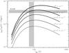 |
Fig. 6 [Cii]λ 158 μm to FIR intensity ratio as a function of the gas temperature for different constant gas thermal pressures. The [Cii] cooling is computed from Eq. (2) and the FIR flux from the integration of our dust model over the range 42 − 122 μm (with a radiation field G0 = 9, see Sect. 4.2 and Fig. 5). The observed ratio for 3C 326N, I[CII]/IFIR(42 − 122 μm) = 0.035 ± 0.014 is indicated by the horizontal dotted line and the grey area represents the uncertainty, dominated by the large error on the SPIRE measurements. The vertical grey bar displays the range of gas temperatures as constrained by observations of the [Cii] to [Oi]63 μm line ratio (see Fig. 7 and Sect. 4.3). For this range of gas temperatures of 70 <T< 100 K, the range of pressures that matches both observational constraints is P/k ≈ 7 × 10⁴ − 2 × 10⁵ K cm-3. |
 |
Fig. 7 Collisional calculation of the ratio of the [Cii]λ 158 μm to [Oi]λ 63 μm line intensity ratio in the temperature versus density plane. The dashed lines indicate constant values of the gas thermal pressure. The observed [Cii] to [Oi]63 μm ratio in 3C 326N [Cii]/[Oi] |

To estimate the total dust mass, we fit the IR spectral energy distribution (SED) (MIPS+PACS+SPIRE) of 3C 326N with the DustEm dust model (Compiègne et al. 2011), using the IDL DustEm wrapper4. The measured FIR fluxes are given in Table 2. The only free parameters are the radiation field intensity, G0, and the different natures of dust grains. We use Galactic mass fractions of the dust grains populations. This may not be entirely correct for such a powerful radio galaxy, but this assumption does not significantly affect our estimate of the total mass since we are mainly focusing on the FIR emission coming from large grains. The results are shown on Fig. 5, where we focus on the FIR part of the SED because we are only interested here in the total dust mass.
From the DustEm fit we constrain the radiation field to be G0 = 9 ± 1, and a total dust mass of Mdust = 1.1 × 10⁷ M⊙. For a dust-to-gas mass ratio of 0.007, this translates into a total gas mass of Mgas = 1.6 × 10⁹ M⊙. Despite the very low star-formation rate in 3C 326N (≤0.07 M⊙ yr-1 from PAH and 24μm measurements, Ogle et al. 2007), this radiation field is of the order of magnitude of the UV field derived from GALEX measurements ( , Ogle et al. 2010), and is mainly due to the old stellar population. We compared our DustEm modeling with the Draine & Li (2007) dust model. If we adopt G0 = 9, we find Mtot(H2) = 1.2 × 10⁹ M⊙. For comparison, had we adopted G0 = 2, we would have found Mgas = 2.9 × 10⁹ M⊙. This shows that the total gas mass inferred from the modeling of the dust emission does not depend strongly on G0.
This total mass of gas derived from the modeling of the dust FIR SED is roughly in agreement with the mass of warm H2 gas inferred from the fit of the pure-rotational H2 excitation diagram (2.7 × 10⁹ M⊙, including He, Ogle et al. 2010), and matches the mass of molecular gas derived from the CO(1−0) line measurement (2 × 10⁹ M⊙Nesvadba et al. 2010). This good correspondence indicates that most of the gas mass in 3C 326N is molecular.
4.3. Constraints on the physical state of the gas: [CII] as a probe of the warm, low pressure molecular gas
In this section we combine the [Cii] cooling rate calculation (Sect. 4.1) with the dust modeling (Sect. 4.2) to constrain the physical conditions (pressure) of the gas required to account for the observed [Cii] luminosity. We compute the ratio of [Cii] line emission to FIR dust emission as a function of the thermal gas pressure, under the same assumptions given in Sect. 4.1. We showed in Sect. 4.1 that the [Cii] line emission traces mostly warm molecular gas. So again we compute the [Cii] cooling rate assuming that 90% of the gas is in molecular form, and 10% is atomic, with an electron fraction dominated by Carbon ionization. Figure 6 shows the expected ratio of the [Cii] to FIR flux for a range of gas thermal pressures between P/k = 2.5 × 104 cm-3 K and 4 × 105 cm-3 K, and temperatures T = 10 − 1000 K, with P/kT = nH. The FIR flux is computed from the dust model discussed in Sect. 4.2 and shown in Fig. 5, after integration over the wavelength range 42−122μm (as commonly used for extragalactic studies, e.g., Helou et al. 1988; Stacey et al. 2010). We find a FIR luminosity of LFIR(42 − 122 μm) = 2.0 ± 0.8 × 10⁹ L⊙. The curves in Fig. 6 peak at ≈ 100 K, close to the excitation temperature of the upper level J = 3/2 of the transition. At this temperature, optimal for [Cii] excitation, the observed line-to-continuum ratio is matched for a range of pressures 7 × 10⁴<P/k< 2 × 10⁵ K cm-3.
For the total gas mass inferred from the modeling of the dust FIR continuum (1.6 × 10⁹ M⊙), this corresponds to a [Cii] cooling rate λC+ = 1.4 × 10⁻²⁵ erg s-1H-1 for our estimate of G0 ≈ 9. This is a factor 5 higher than for the diffuse ISM in the Milky Way (2.6 × 10⁻²⁶erg s-1 H-1, Bennett et al. 1994).
To help in breaking the degeneracy between temperature and density, we use the Herschel/PACS observations of the [Oi]λ63 μm line with ![Mathematical equation: \hbox{$F([{\rm OI}]) = 5.5_{-0.22}^{+0.07} \times 10^{-18} \, $}](/articles/aa/full_html/2015/02/aa23612-14/aa23612-14-eq190.png) W m-2. The [Oi] data are part of a separate program – P.I. Ogle –, and the spectrum will be published in a separate paper as part of a larger sample of radio-galaxies (Guillard et al. 2014). The uncertainty on the [Cii]-to-[Oi] line flux ratio is dominated by the low signal-to-noise [Oi] detection. Figure 7 shows the results of collisional excitation calculation of the [Cii]-to-[Oi] line intensity ratio in the temperature versus density plane. The cooling from [Cii] is computed from Eq. (2) and for the [Oi] cooling we solve the three-level fine-structure O(3P) oxygen system. We considered collisions with H, H2 and electrons. We use the O(3P)-H collisional rate coefficients computed by Abrahamsson et al. (2007) which we fitted as a function of the temperature to get analytical expressions. The rate coefficients for collisions with H2 are taken from Jaquet et al. (1992), and those with electrons are from Bell et al. (1998). These calculations show that the gas temperature is well constrained by the [Cii]-to-[Oi] line ratio. The comparison of these calculations with the observed [Cii]-to-[Oi] ratio shows that, for the range of pressures matching the observed [Cii]-to-FIR ratio (Fig. 6), the average density of the gas has to be relatively low, within the range 7 × 10²<nH< 3 × 103 cm-3 (Fig. 7).
W m-2. The [Oi] data are part of a separate program – P.I. Ogle –, and the spectrum will be published in a separate paper as part of a larger sample of radio-galaxies (Guillard et al. 2014). The uncertainty on the [Cii]-to-[Oi] line flux ratio is dominated by the low signal-to-noise [Oi] detection. Figure 7 shows the results of collisional excitation calculation of the [Cii]-to-[Oi] line intensity ratio in the temperature versus density plane. The cooling from [Cii] is computed from Eq. (2) and for the [Oi] cooling we solve the three-level fine-structure O(3P) oxygen system. We considered collisions with H, H2 and electrons. We use the O(3P)-H collisional rate coefficients computed by Abrahamsson et al. (2007) which we fitted as a function of the temperature to get analytical expressions. The rate coefficients for collisions with H2 are taken from Jaquet et al. (1992), and those with electrons are from Bell et al. (1998). These calculations show that the gas temperature is well constrained by the [Cii]-to-[Oi] line ratio. The comparison of these calculations with the observed [Cii]-to-[Oi] ratio shows that, for the range of pressures matching the observed [Cii]-to-FIR ratio (Fig. 6), the average density of the gas has to be relatively low, within the range 7 × 10²<nH< 3 × 103 cm-3 (Fig. 7).
In addition, the fitting of the rotational H2 line emission with a thermal equilibrium model shows that the bulk of the warm H2 gas must be at a temperature of ≈ 100 K to match the observed luminosity in the low-J H2 rotational lines, i.e., 0−0S(0) and 0−0S(1), (e.g., Ogle et al. 2010; Guillard et al. 2012). Both constraints on the warm H2 density (7 × 10²<nH< 3 × 103 cm-3) and temperature (70 <T< 100 K) rule out the possibility that the [Cii] emission is coming from a lower fraction of the gas mass at higher pressure, because the [Cii]-to-FIR flux ratio is dropping as the temperature deviates from 100 K (Fig. 6). Furthermore, since dense, high-pressure gas would be luminous in the CO lines, further constraints on the gas density can be obtained from CO observations. A preliminary inspection of the SPIRE FTS spectrum of 3C 326N shows no detection of high-J CO lines (P. Ogle, priv. comm.), which seems to confirm that the molecular gas has a low average density or a low filling fraction of dense gas. We conclude that the average pressure of the warm H2 gas in 3C 326N is P/k ≈ 105K cm-3, with a temperature of T ≈ 100 K and a density nH ≈ 103 cm-3. Therefore, in 3C 326N, the MIR rotational lines of H2 and the [Cii] line trace the same warm molecular gas.
5. What is the heating source of the gas?
5.1. An extreme [CII] line luminosity
In Sect. 4.3, we computed a [Cii] to FIR flux ratio of I[CII]/IFIR(42 − 122 μm) = 0.035 ± 0.014, see Fig. 6. This is unusually high, a factor of 3 to 5 more than what is observed in typical star-forming galaxies (Malhotra et al. 2001; Stacey et al. 2010; Díaz-Santos et al. 2013; Rigopoulou et al. 2014; Herrera-Camus et al. 2014). This ratio is very similar to what is found in the shocked intergalactic medium of the Stephan’s Quintet galaxy collision (0.04–0.08, Appleton et al. 2013), and, to a lower extent, in the HCG 57 group (up to 0.017, Alatalo et al. 2014a). As we see in this section, the [Cii] emission in 3C 326N cannot be powered by star formation.
We demonstrated in Sect. 4 that the [Cii] line luminosity in 3C 326N implies that a significant fraction (30–50%) of the molecular gas mass (5.5 − 9.5 × 10⁸ M⊙) has to be warm (70 <T< 100 K). In the following sections, we discuss the potential heating sources of this gas.
Ogle et al. (2010) and Nesvadba et al. (2010) ruled out UV and X-rays as possible sources for the heating of the warm H2 gas in 3C 326N. Since we demonstrated that most of the [Cii] line emission is coming from the warm molecular gas, this is a fortiori valid for the [Cii] excitation. Furthermore, the [Cii] to PAH luminosity ratio is too high ([Cii]/PAH 7.7 μm > 2.5) to be accounted for solely by photoelectric heating (Guillard et al. 2013), which rules out photon heating as the main source for the [Cii] emission. Therefore, the two remaining possible heating sources of the gas in 3C 326N are the turbulent heating and the cosmic rays.
5.2. Turbulent heating
Dissipation of turbulent energy (mechanical heating) has a strong impact on the excitation conditions and physical state of the diffuse ISM and molecular gas in galaxies (e.g., Godard et al. 2014; Kazandjian et al. 2012; Rosenberg et al. 2014). Nesvadba et al. (2010) argue that the dissipation of mechanical energy is the most likely excitation source of the molecular gas in 3C 326N. This turbulence must be sustained by a vigorous energy source because the radiative cooling time of the warm molecular gas is short (≈ 104 yr; Guillard et al. 2009). They demonstrate that a few percent of the jet kinetic luminosity (at least a few 1044 erg s-1) deposited into the gas is sufficient to drive the outflow and power the observed H2 and Hii line luminosity, which makes jet kinetic energy a plausible source for the heating of the molecular gas.
Within this framework, [Cii] line observations allow us to build a more complete mass and energy budget. In particular, we update the estimate of the turbulent gas velocity dispersion σturb required to balance the total [Cii] + H2 line cooling rate. Turbulent heating is energetically possible if the total turbulent kinetic luminosity is greater than the observed line luminosity: ![Mathematical equation: \begin{equation} \label{eq:turb_heat_rate} \dfrac{3}{2} M_{\rm tot}({\rm H_2}) \frac{\sigma _{\rm turb} ^3}{H_{\rm g}} > L_{\rm [CII]} + L_{\rm H_2} , \end{equation}](/articles/aa/full_html/2015/02/aa23612-14/aa23612-14-eq206.png) (5)where Mtot(H2) = 2 × 10⁹ M⊙ is the total molecular gas mass, σturb is the turbulent velocity dispersion, and Hg the characteristic injection scale of the turbulence, which we assume to be the vertical scale height of the gas (see Sect. 7 for a discussion of that assumption). The minimal velocity dispersion required to balance the line cooling is thus given by
(5)where Mtot(H2) = 2 × 10⁹ M⊙ is the total molecular gas mass, σturb is the turbulent velocity dispersion, and Hg the characteristic injection scale of the turbulence, which we assume to be the vertical scale height of the gas (see Sect. 7 for a discussion of that assumption). The minimal velocity dispersion required to balance the line cooling is thus given by ![Mathematical equation: \begin{equation} \label{eq:min_vel_disp} \sigma _{\rm turb} > 90 \ \left( \frac{ L_{\rm [CII]+H_2}/M_{\rm tot}}{0.18 \ L_{\odot}/M_{\odot}}\right)^{1/3} \left( \frac{H_{\rm g}}{1\, {\rm kpc}} \right)^{1/3} \ \ \rm{km \ s^{-1}} . \end{equation}](/articles/aa/full_html/2015/02/aa23612-14/aa23612-14-eq209.png) (6)The observed [Cii]λ158 μm line cooling rate per unit mass in 3C 326N is L[CII]/Mtot(H2) = 0.044 ± 0.006 L⊙/M⊙, and the H2 rotational line cooling rate is LH2/Mtot(H2) = 0.14 ± 0.02 L⊙/M⊙ (Ogle et al. 2010). In Eq. (6) we chose to compute the minimal velocity dispersion for a relatively large vertical scale height, Hg = 1 kpc. This scale height is within the range of gas scale heights we constrain in Sect. 7 and is comparable to the radius of the molecular disk seen in ro-vibrational H2 line emission (Nesvadba et al. 2011). For those values of cooling rate and scale height, we obtain σturb> 90 km s-1.
(6)The observed [Cii]λ158 μm line cooling rate per unit mass in 3C 326N is L[CII]/Mtot(H2) = 0.044 ± 0.006 L⊙/M⊙, and the H2 rotational line cooling rate is LH2/Mtot(H2) = 0.14 ± 0.02 L⊙/M⊙ (Ogle et al. 2010). In Eq. (6) we chose to compute the minimal velocity dispersion for a relatively large vertical scale height, Hg = 1 kpc. This scale height is within the range of gas scale heights we constrain in Sect. 7 and is comparable to the radius of the molecular disk seen in ro-vibrational H2 line emission (Nesvadba et al. 2011). For those values of cooling rate and scale height, we obtain σturb> 90 km s-1.
Our [Cii] data, as well as NIR H2 measurements, show that the observed gas velocity dispersions are within the range 160 <σ< 350 km s-1 (from the linewidth measurements of the individual velocity components). Based on the analysis of the H2 line velocity maps, Nesvadba et al. (2011) estimate ratios of circular-to-turbulent velocities vc/σ = 0.9 − 1.7. This ratio is likely to be underestimated (by ≈15%, Nesvadba et al. 2011) because of the effect of beam-smearing5. Beam smearing strongly affects the determinations of the velocity structure in the data by transforming what are in reality circular motions into apparent higher velocity dispersions. Taking beam smearing into account, Nesvadba et al. (2011) show that the contribution of the systematic rotation to the line width is σrot ≈ 100 km s-1. By subtracting in quadrature the contribution of the rotation to the observed σ from [Cii] data, we find that the turbulent velocity dispersions in 3C 326N are within the range 120 <σturb< 330 km s-1. Therefore, the energetic condition given above in Eq. (5) is satisfied, even for high values of the scale height. The turbulent kinetic luminosity associated with the H2 gas velocity dispersion alone on the physical scale of the disk is at least a factor of 2 higher than the total [Cii]+H2 cooling rate.
As argued in previous papers (Guillard et al. 2009; Nesvadba et al. 2010), shocks are responsible for the dissipation of a large percentage of the total kinetic energy in H2-luminous galaxies, but most of the kinetic energy dissipation does not occur within the ionized gas through dissociative shocks. It occurs mostly in non-dissociative, low-velocity C-shocks (velocities lower than 40 km s-1). Since the kinetic energy is mostly dissipated in the molecular gas, molecular viscosity causes the turbulent dissipation. The timescale associated with the turbulent energy dissipation timescale is given by ![Mathematical equation: \begin{equation} \label{eq:turb_diss_time} \tau _{\rm diss} \approx 5\times 10^7 \left( \frac{\sigma _{\rm turb}}{200\ \rm km \ s^{-1}} \right)^2 \left( \frac{0.18 \ L_{\odot}/M_{\odot}}{ L_{\rm [CII]+H_2}/M_{\rm tot}(\rm H_2)} \right)\ \rm \ [yr]. \end{equation}](/articles/aa/full_html/2015/02/aa23612-14/aa23612-14-eq219.png) (7)Given the range of turbulent velocity dispersion inferred above, the dissipation time ranges between 2 × 10⁷ and 1.5 × 10⁸ yr. Therefore, the dissipation time is comparable to or longer than the lifetime of the radio jet or the duty cycle of the jet activity. The dissipation of turbulent energy in 3C 326N can power the line emission coming from the molecular gas between the times when the jet is active.
(7)Given the range of turbulent velocity dispersion inferred above, the dissipation time ranges between 2 × 10⁷ and 1.5 × 10⁸ yr. Therefore, the dissipation time is comparable to or longer than the lifetime of the radio jet or the duty cycle of the jet activity. The dissipation of turbulent energy in 3C 326N can power the line emission coming from the molecular gas between the times when the jet is active.
We also define ϵ as the ratio between the total [Cii]+H2 luminosity and the turbulent heating rate. Within the framework given by the above condition (Eq. (5)), ϵ< 1, which means that not all the turbulent energy dissipated is radiated into the [Cii] and H2 lines. Then Eq. (5) can be rewritten as a relationship between the gas scale height and the gas velocity dispersion: ![Mathematical equation: \begin{equation} \label{eq:sca_hei_turb_diss} H_{\rm g} = \frac{3}{2}\, \epsilon \, \sigma _{\rm turb} ^{3} \left( \frac{L_{\rm [CII]+H_2}}{M_{\rm tot}(\rm H_2)} \right)^{-1} \cdot \end{equation}](/articles/aa/full_html/2015/02/aa23612-14/aa23612-14-eq224.png) (8)We use this relation in Sect. 7 to discuss the dynamical state of the gas in the disk of 3C 326N.
(8)We use this relation in Sect. 7 to discuss the dynamical state of the gas in the disk of 3C 326N.
5.3. Heating by cosmic rays
We compute here the cosmic ray ionization rate required to balance the [Cii]+H2 line cooling rate. The gas cooling rate through the [Cii] line and the H2 rotational lines of 4π (I(CII) + I(H2)) /NH = 4.4 × 10⁻²⁵ erg s-1 H-1. The heating energy deposited per ionization is ~13 eV for H2 gas (Glassgold et al. 2012). Thus, to heat the gas, a cosmic ray ionization rate of ζH2 = 2 × 10-14 s-1 is needed. This required ionization rate is a factor about 60 larger than in the diffuse interstellar gas of the Milky Way (Indriolo & McCall 2012), and a factor of 18 greater than the value derived for the gas near the galactic center (Goto et al. 2013).
However, each ionization produces two ions and one H2 dissociation, so the gas has to be dense enough to reform H2 and be mostly molecular. The formation rate (ΓH2n(HI)n(H)) should balance the destruction rate ζ/n(H2) of H2. This balance is written ΓH2 = ζH2fH2/ (1 − fH2)/2 /n(H) where fH2 = 2 n(H2) /n(H) is the molecular fraction of the gas. As a result, the condition for the gas to be predominately molecular can be written as ![Mathematical equation: \begin{equation} n_{\rm H} \geqslant \frac{\zeta_{\rm H_2} \times f_{\rm H_2}}{\Gamma_{\rm H_2} \times 2 (1 - f_{\rm H_2})} = 3.3 \times 10^2 \frac{f_{\rm H_2}}{1 - f_{\rm H_2}}\ \rm [cm^{-3}] , \end{equation}](/articles/aa/full_html/2015/02/aa23612-14/aa23612-14-eq231.png) (9)if we adopt the canonical value of ΓH2 ≈ 3 × 10-17 cm3 s-1 (e.g., Gry et al. 2002; Habart et al. 2004), and the cosmic ray ionization rate derived above (ζ = 2 × 10-14 s-1). For a gas that is mostly molecular (fH2 = 0.9), we find that
(9)if we adopt the canonical value of ΓH2 ≈ 3 × 10-17 cm3 s-1 (e.g., Gry et al. 2002; Habart et al. 2004), and the cosmic ray ionization rate derived above (ζ = 2 × 10-14 s-1). For a gas that is mostly molecular (fH2 = 0.9), we find that  cm-3. This lower limit on the gas density corresponds to the upper boundary of the gas density range derived from the observed [Cii]-to-[Oi] line ratio (Fig. 7).
The average gas density derived from [Cii], [Oi], and FIR continuum photometry (7 × 10²<nH< 3 × 103 cm-3, see Sect. 4.3) does not permit a high H2 re-formation rate and thus these conditions are not favorable for keeping the gas molecular in the presence of intense cosmic ray radiation. We therefore do not favor cosmic rays for playing a dominant role in the heating and excitation of the molecular gas. However, the lower limit on the gas density derived above is close enough to the estimated range of densities (Fig. 7) that it is not possible to conclusively rule out the cosmic ray heating, provided that such a high ionization rate can be maintained on the large scale of the galaxy’s interstellar medium. We do not have strong constraints on the diffuse cosmic ray intensity in radio galaxies, which may be enhanced if the jets flare (Biermann & de Souza 2012; Laing & Bridle 2013; Meli & Biermann 2013) but could also be low in the absence of star formation as is observed in 3C 326N.
Because they penetrate deeper than UV photons into molecular clouds, cosmic rays may play an important chemical role in dissociating CO molecules (via secondary photons), thus maintaining a high C+/ CO fractional abundance. Mashian et al. (2013) have indeed shown that in nH2 = 103 cm-3, T = 160 K, UV-shielded gas, the gas can be molecular (1 <nH2/nH< 50) with n(C+) /n(CO) ≈ 0.8 for 3 × 10-16<ζ< 10-14 s-1. While cosmic rays may not play a dominant role in heating and exciting the molecular gas, they very likely play an important role in the chemistry of the gas.
6. Outflow and turbulence in 3C 326N
In this section we discuss the two phenomena that can make the [Cii] line profile very broad and skewed (see Fig. 1): a massive outflow and turbulence. These two processes are at work in 3C 326N and are coupled, since the outflow is likely to power some of the turbulence within all phases of the gas.
6.1. The wind and outflow rates in 3C 326N
Since the [Cii] line emission traces ≈ 30% of the total molecular gas mass in 3C 326N (Sect. 4), associating the broad wing with an outflow component would require that a large amount of the neutral medium is outflowing. The blueshifted wing accounts for 35% of the total [Cii] line flux (Table 1). To estimate the fraction of the gas mass that is actually outflowing and escaping from the galaxy, we integrate the [Cii] line profile from the highest observed velocity in the [Cii] line (−1000 km s-1) to the estimate of the escape velocity at the largest H2 radius (−400 km s-1, Nesvadba et al. 2011). Assuming that the C+ excitation and abundance are the same in the disk and in the outflow, we find that this fraction is 11 ± 2%, corresponding to a total mass of outflowing gas of 1.8 ± 0.3 × 10⁸ M⊙.
Using the upper limit of the size of the [Cii] emitting region, the 10′′ PSF of PACS, and a Doppler parameter of 350 km s-1 for the wind (Nesvadba et al. 2010), we estimate the dynamical time of the outflow to be lower than 107 yrs. This gives a lower limit for the outflow rate of > 20 M⊙ yr-1 and an upper limit on the depletion time of < 108 yrs. Such a timescale is longer than or comparable to the lifetime of the radio jet (107 − 108 yrs, Willis & Strom 1978) and comparable to the orbital timescale (≈ 3 × 10⁷ yrs, Nesvadba et al. 2011).
The outflow rate we estimate from the [Cii] emission is about half the mass outflow rate of neutral gas estimated from Na D absorption, 40−50 M⊙ yr-1 (Nesvadba et al. 2010), although the Na D absorption extends to higher terminal velocities, up to v = −1800 km s-1, and is therefore likely to sample gas that we do not detect in [Cii]. The reason for this difference may be either observational, in the sense that our PACS data do not have the signal-to-noise ratio needed to probe the full velocity range of the wind, or astrophysical, since the Na D absorption line could probe gas down to lower column densities, including gas that is more readily accelerated. If the mass outflow rate in 3C 326N is as high as 20 − 50 M⊙ yr-1, this means that we are observing this galaxy at a very specific and brief time in its evolution, and one can wonder why we would observe a gas disk at all with such a short depletion timescale. Comparable mass outflow rates driven by AGN have been reported by, for example, Morganti et al. (2013a), McNamara et al. (2014) and García-Burillo et al. (2014). To replenish the disk, the inflow rate would need to be comparable to the outflow rate on at least the orbital timescale, which is comparable to the mass deposition rates observed in galaxy clusters (e.g., Bregman et al. 2005; Fabian et al. 2005) and which seems very high and unlikely for such an isolated galaxy. Therefore, we conclude that AGN with such high relative mass outflow rates are a transient phenomenon, which we are able to detect because radio galaxies (and quasars) are, by selection, caught in a very specific and short phase of their life. This result is in agreement with the low detection rate of the occurrence of Hi outflows seen in absorption (Gereb et al. 2015).
In 3C 326N, the [Cii] line is unlikely to suffer significantly from opacity effects6. If the broad wing component of the [Cii] line traces the cold outflowing gas, then why is the line asymmetric? The spatial distribution of the outflowing gas, and the distribution of the filling factor of the cold gas are unlikely to be homogeneous and isotropic, which could skew line profiles. Asymmetric Hi absorption line profiles associated with off-nuclear outflows are indeed observed in radio galaxies (e.g., Morganti et al. 2005a; Gereb et al. 2015). In fact, the high degree of symmetry seen in the broad line profiles towards e.g., high-redshift quasars (Maiolino et al. 2012), and often interpreted as outflows, is remarkable. The complex geometry of the gas distribution also increases the uncertainty on the estimates of the mass outflow rates.
6.2. Line wings and turbulence on large scales
Turbulence within the entire gas disk could also broaden and skew the [Cii] line profile, making the line wing prominent. In addition to rotation and outflow, the line profiles in 3C 326N may also trace the stochastic injection of turbulent energy on large scales by the radio jet into the gas. If this contribution is important, our estimates of mass outflow rates could be significantly over-estimated (see also Mahony et al. 2013, for the contribution of turbulence to the broad Hi absorption profile observed in 3C 293).
Because the largest eddies are rare in space and time, they are not well statistically sampled by the observations, which causes irregularities in the line profiles. In such a perspective where the turbulence is driven by the radio jet, numerical simulations suggest that the backflow of the jet can inject turbulent energy into the gas over the vertical scale height of the disk (Gaibler et al. 2012). Therefore, the largest turbulent cells are likely to be a few kpc in size, and the number of correlation lengths is small, possibly explaining why the spectral line profiles are jagged. This could mimic outflowing gas, but, because those velocity structures are short-lived and chaotic, the gas actually does not have the time to escape out of the galaxy.
The line profiles observed in 3C 326N are very reminiscent of what is observed in the spectral line shapes (e.g., CO) of Galactic molecular clouds, where their irregularities can be a signature of the statistical properties of turbulence (Falgarone & Phillips 1990; Falgarone et al. 1992). Studies of the probability density distributions of the velocity field (or vorticity, pressure, or energy dissipation rate) in the Galactic ISM show that their non-Gaussian behavior could in fact be a consequence of stochasticity on small scales (see Hily-Blant et al. 2008, for observational evidence of intermittency).
7. Dynamical state of the molecular gas in the 3C 326N disk
In this section we discuss the impact of turbulence on the dynamical state of the molecular gas and star formation. We investigate if our interpretation of the H2 and [Cii] line emission, as tracers of turbulent energy dissipation, fits with a plausible dynamical state of the molecular gas in 3C 326N.
The hydrostatic equilibrium condition between the gas plus stellar gravity and the total (thermal plus turbulent) gas velocity dispersion determines the vertical scale height of the disk (e.g., Lockman & Gehman 1991; Malhotra 1994). In 3C 326N, we expect that turbulent support of gas in the vertical gravitational field is important. In order to determine if the disk is self-gravitating or not, we calculate the balance between the turbulent pressure gradient and the gravity (in the vertical direction perpendicular to the disk plane) and we derive an expression for the vertical scale height. Then we investigate if such an expression can be reconciled with the expression of the scale height constrained from the balance between the turbulent heating rate and the observed [Cii]+H2 cooling rate.
Because the jet is roughly perpendicular to the orientation of the disk (Rawlings et al. 1990), it is likely that energy is being transferred through turbulence generated by the over-pressured hot gas created by the heating of the jet. This gas is also produced in models of relativistic jets as they expand into the surrounding medium (e.g., Gaibler et al. 2011; Wagner et al. 2012). As in Sect. 5, the scale of injection of kinetic energy is comparable to the vertical scale height of the gas in the disk, Hg. This is a reasonable assumption as the Mpc-size of the radio emission is much larger than the size of the disk.
The turbulent pressure can be written as 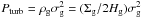 , where ρg is the average mid-plane gas mass density, Σg the gas mass surface density, Hg the gas vertical scale height, and σg is the vertical gas velocity dispersion7. The pressure in the disk plane due to the gas and stellar gravity can be written as
 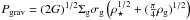 (Blitz & Rosolowsky 2004; Ostriker et al. 2010), where ρ⋆ is the stellar mass density and G the gravitational constant. The vertical equilibrium condition between the turbulent pressure gradient and the gravity has two limiting forms.
We first consider the case where the stellar gravity dominates over the gas gravity in the disk, i.e. ρ⋆ ≫ ρg. This is likely to be the case for 3C 326N since the stellar mass (M⋆ ≈ 3 × 10¹¹ M⊙) is much higher than the total gas mass (Mg ≈ 2 × 10⁹ M⊙). In this “star-dominated disk”, the gravitational force per unit mass of gas along z is constant. Then, the gas scale height is proportional to the velocity dispersion of the gas:  (10)where H⋆ is the stellar vertical scale height. This expression is plotted in Fig. 8 as the solid lines. The parametrization of the stellar morphology, based on our examination of SDSS images8, is uncertain, since we do not know the flattening of the stellar distribution in 3C 326N. Therefore, we plot Eq. (10) for four different parametrizations that bracket the possible range of stellar scale heights, H⋆ = 0.3 − 3 kpc, and stellar mass surface densities, Σ⋆ = 320 − 950 M⊙ pc-2, which corresponds to stellar masses M⋆ = 1 − 3 × 10¹¹ M⊙ in a sphere of diameter 20 kpc.
Figure 8 displays the expression of the scale height constrained by the balance between the turbulent heating rate and the observed line cooling rate, given in Eq. (8). Equation (8) is plotted as the dashed lines for two values of the ϵ parameter (ϵ = 1 means that 100% of the turbulent energy dissipated is radiated into the [Cii] and H2 lines). The grey area in Fig. 8 shows the plausible parameter space if the gas is within the stellar disk: the gas velocity dispersion would lie within the range 60 <σg< 190 km s-1, and the gas scale height would be comprised within 0.3 <Hg< 4 kpc. This is a plausible solution if 3C 326N is a lenticular galaxy. We note that gas scale height above H⋆ = 3 kpc are unphysical since in that case the stars dominate the gravitational potential in the disk.
Then, we consider the case of a self-gravitating gas disk in a stellar spheroid morphology, where the gravity is dominated by the gas on the scale of the vertical height of the disk (ρg ≫ ρ⋆). Equating Pgrav = Pturb, we find that the gas scale height can be simplified as:  (11)For the sake of clarity, and because this limiting form is unlikely for 3C 326N (M⋆ ≫ Mg, see above), we do not plot this case in Fig. 8. For the observed value of gas mass surface density in 3C 326N (Σg = 100 M⊙ pc-2), the self-gravitating disk curve would intercept the turbulent dissipation solution (dashed lines) at gas scale heights much larger than the size of the galaxy (500 − 900 kpc for ϵ = 0.5 − 1 and L[CII] + H2/MH2 = 0.18 L⊙
 ). This shows that we cannot reconcile the observed turbulent heating rate with the hypothesis of a self-gravitating disk.
We also consider the case of an elliptical galaxy where the H2 gas is bound by the gravitational binding energy of the stellar spheroid  , where r is the spheroid radius. We find that the equivalent external pressure on the gas is
  . For a radius of 10 kpc, Pext/k = 2 × 10⁶ K cm-3. This pressure is comparable to the turbulent pressure
  observed on the scale of the disk (Pext/k = 0.8 × 10⁶ K cm-3 for Hg = 3 kpc and σg = 100 km s-1), and an order of magnitude higher than the average thermal pressure of the warm H2 gas deduced from the [Cii] observations (105 K cm-3, see Sect. 4.3). Therefore, the corresponding expression of the gas scale height, not plotted in Fig. 8, would intercept the dashed curves of the turbulent dissipation solution at locations very similar to the lenticular (“star-dominated disk”) solution (grey area).
In conclusion, finding a dynamical state of the gas compatible with our interpretation where turbulent heating is the main heating source of the molecular gas in 3C 326N and where the H2 and [Cii] lines are powered by the dissipation of the gas turbulent kinetic energy, implies large vertical gas velocity dispersions (60 <σg< 190 km s-1) and high values for the gas scale height (0.3 <Hg< 4 kpc). It is plausible to find a such high vertical gas velocity dispersion in 3C 326N given the observed turbulent velocity dispersion estimated in Sect. 5.2 (120 <σturb< 330 km s-1). From the NIR H2 line morphology, the H2 disk has to have a thickness Hg< 0.9 kpc (Nesvadba et al. 2011). However, the NIR ro-vibrational H2 lines trace denser and warmer gas than the [Cii] line, accounting for a small fraction of the total H2 mass, so the [Cii]-emitting disk may be larger. The SINFONI observations also have a limited surface brightness sensitivity, so we may not see all the warm H2 disk.
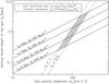 |
Fig. 8 Vertical scale height as a function of the gas vertical velocity dispersion. The solid lines are computed for the “star-dominated disk” limiting form of the hydrostatic equilibrium in the disk plane (Eq. (10)) plotted for a range of possible values of the stellar disk parametrization H⋆ = 0.3 − 3 kpc and Σ⋆ = 320 − 950 M⊙ pc-2. The dashed lines plot the scale height values given by the balance between the turbulent heating rate and the observed [Cii]+H2 line cooling rate (Eq. (8)), for two values of the efficiency parameter ϵ (50% and 100%, see Sect. 7 for details). The grey area shows the plausible (σg, Hg) parameter space for the 3C 326N gas disk. |
8. Discussion: turbulence as a feedback mechanism
In this section we discuss some general implications of the work presented in this paper for galaxy evolution.
The [Cii] profile we observe in 3C 326N exhibits very broad wings, especially toward the blue where the velocities reach up to about −1000 km s-1. Such high velocities are typically interpreted as terminal velocities of energetic outflows. Because of the relatively high densities necessary for observing strong [Cii] emission (e.g., Maiolino et al. 2012), CO emission and absorption (e.g., Feruglio et al. 2010; Dasyra & Combes 2012; Cicone et al. 2012, 2014; Morganti et al. 2013b), and molecular absorption lines (e.g., Aalto et al. 2012; Spoon et al. 2013), large mass ejection rates have usually been derived from these outflow velocities.
These high gas velocities are consistent with the velocities modeled in jet interactions with gas disks surrounding an AGN (Gaibler et al. 2012; Wagner et al. 2012, 2013). In these simulations, the high gas velocities are, however, associated with gas at lower densities than we observe in the [Cii] emitting gas (Gaibler et al. 2012). Getting agreement between the velocities of the different gas phases requires the warm molecular gas to be formed in the turbulent backflow of the jet, and its formation of molecular gas could be triggered by the compression generated by the two-sided radio jet. If so, this implies that not only does the jet play a crucial role in energizing the turbulent cascade, but in fact it is also responsible for the physical state (predominately molecular instead of hot ionized or warm neutral medium) and the distribution of the molecular gas (its disk-like structure). Despite the high velocities observed in the wings of the line profiles of [Cii] and the ro-vibrational lines of H2, the molecular gas is perhaps confined by the pressure of the hot halo gas with which the jet is strongly interacting.
A natural outcome of this picture is that the gaseous disks in radio galaxies should be approximately perpendicular to the jet axis (de Koff et al. 1996, 2000; Martel et al. 1999; Carilli & Taylor 2000), although many sources would show more complex gas distributions depending on the phase probed or the symmetries in the jets. Moreover, if the jets of the AGN shut down, the phase and structure of the disk will change dramatically, perhaps even experiencing a phase transition from a molecular phase to a hot ionized phase.
In addition, the picture of a highly turbulent molecular disk may also explain one of the most significant puzzles in relation to outflows from AGN, namely, the apparent short gas “erosion” timescales in some of the sources, less than ≈10 Myrs. A large percentage of the AGN population show such short timescales (e.g., Feruglio et al. 2010; Nesvadba et al. 2011; Cicone et al. 2014). In fact, Nesvadba et al. (2011) find that the erosion timescale of the 3C 326N disk was about that of the orbital timescale, which roughly agrees with our estimate (3 − 10 × 107 yrs). These findings beg the question: why do we see outflows and gas disks at all in these sources? Either the outflow duty cycle is short and the gas replenished quickly, or the erosion timescales are wrong (for example, the total mass estimated or the underlying model for estimating the outflow rate; Alatalo et al. 2011; Alatalo et al. 2014b).
As we discussed earlier, the interaction between the backflow, generated by the propagating jets, and the disk can create high turbulent velocities, in the range 100 − 1000 km s-1 (Gaibler et al. 2012). Because the broad line wings have several times the velocity dispersion of the majority of the gas, they could be the signature of the stochastic nature of turbulence (see, for example, Falgarone & Phillips 1990; Pety & Falgarone 2003). Since the pressure of the overlying hot gas is probably several times that of the disk itself (Gaibler et al. 2012), this high velocity gas is confined and not outflowing because it is generated by the interaction with the hot gas phase and can be naturally related to the turbulent cascade, depending on the exact source of the high velocity. The high velocities do not necessarily indicate escaping gas and may well be a natural outcome of our overall picture of a high turbulent molecular disk generated by the action of the radio jet on the host ISM and halo gas.
One of the other major implications of these results is that the energy injection from the radio source into the ISM can be both “positive” and “negative” feedback. The feedback is positive in the sense that the over-pressure generated by the jets allows for enhanced formation of H2 gas and the creation of large molecular disks around AGN (Wolfire et al. 1995). However, radio loud AGN may maintain the molecular gas in such a state that it cannot form stars efficiently owing to the high turbulence. Thus we caution against any interpretation of enhanced molecular gas formation around AGN as being systematically a sign of positive feedback in the sense of enhanced star formation.
It appears from our analysis of 3C 326N that while the high compression of the disk resulting from the backflow and turbulence generated by two-sided jets may lead to strong cooling, i.e., enhanced [Cii] emission, and a significant fraction of the gas is molecular, it may also suppress star formation by only allowing a small fraction of the gas to become self-gravitating on any scale. This is probably due to the exceptional turbulent support in 3C 326N, which maintains a very large disk thickness, and is able to stabilize the disk on large spatial scales against fragmentation into bound star-forming clumps of gas. This offers a natural explanation for the quenching of star formation in 3C 326N. The compression may be sufficient to allow small gas clumps to become self-gravitating and collapse to form stars, but not at the rate expected given the gas surface densities observed. We are only suggesting that the star formation efficiency is much lower when the gas phase mixture and physical structure of molecular disks are related by the energy input from radio jets.
This is, however, not to say that in all cases, the action of the jet on a gaseous disk always inhibits star formation. If the disk were pre-existing, rather than being formed by the action of the jet itself as we have proposed, and were composed of gas and stars distributed in a disk, the outcome of the interaction with the backflow might well have been different (e.g., Martig et al. 2013). In disk galaxies, because the stars dominate the baryonic mass distribution, the stellar disk is the main source of (self-)gravity. In such a case, the gas will be initially gravitationally bound and the jet over-pressure may enhance star formation. We suggest this picture to emphasize the role played by self-gravity on large scales. In fact, as we have found, the action of the jet on the surrounding medium is to increase the overall pressure and make the conditions such that high molecular fractions are likely (Wolfire et al. 1995). This may then lead to an enhanced star formation efficiency in disk structure that is already self-gravitating (Silk & Norman 2009; Silk 2013).
9. Summary of results
We detected [Cii]λ 158 μm line emission from the 3C 326N radio galaxy with the Herschel/PACS instrument. The [Cii] is very luminous, twice as bright as the H2 0−0S(1) line detected by the Spitzer IRS. The [Cii]-to-FIR and [Cii] to PAH 7.7 μm flux ratios are extremely high (0.035 ± 0.014 and > 2.5), 3 to 30 times higher than what is observed in typical star-forming galaxies, showing that UV is not the main excitation process.
The [Cii] line profile is broad and asymmetric, with a core of intrinsic FWHM = 340 km s-1, and a pronounced blueshifted wing of FWHM = 800 km s-1. The line is very likely shaped by a mixture of systematic rotation, outflowing gas, and turbulence. We compared the [Cii] kinematics to other tracers to discuss these three relative contributions to the line profile. The [Cii] line matches the NIR H2, Hα, Na D absorption, and CO line profiles well, although these lines probe different phases and mass fractions of the gas. Attributing the line wing to a wind leads to high outflow rates in the range of 20 − 50 M⊙ yr-1, depleting the gas reservoir in timescales of 30 − 100 Myr, within an order of magnitude of the orbital timescale. If true, we are observing this object at a very specific and brief time of its evolution, if the disk is not replenished. These outflow rates may be overestimated because turbulence (generated by the interaction between the disk and the jet’s backflow) can produce short-lived, large velocity increments that contribute to the skewness of the line profile and could mimic outflowing gas.
By combining infrared Spitzer and Herschel photometry and spectroscopy with gas and dust modeling, we inferred the physical and chemical conditions in the [Cii]-emitting gas. We concluded that the [Cii] line emission, like the infrared rotational H2 lines, traces a significant fraction (30 to 50%) of the total mass of molecular gas, which is warm (70 <T< 100 K), and where most of the atomic Carbon is singly ionized. The high observed [Cii] to [Oi] ratio allowed us to constrain the average molecular gas density within the range 700 <nH< 3000 cm-3.
We showed that the most plausible heating source of the molecular gas is the dissipation of supersonic turbulence. This turbulence must be sustained by a vigorous energy source because the radiative cooling time of the warm molecular gas is short (≈ 104 yr). Maintaining this turbulent heating only requires a small percentage of the jet mechanical energy, and the time to dissipate this kinetic energy of the warm molecular gas is about several 10 Myr up to about 100 Myr (Eq. (7)). Cosmic ray heating would require warm H2 densities above 3000 cm-3 for the gas to remain molecular in the presence of cosmic ray ionization. Cosmic rays are therefore not the favored source of heating, but they are very likely to play an important chemical role in maintaining a high C+/CO fractional abundance in the molecular gas. This contrasts with what is normally observed in star-forming galaxies where the gas is heated by photoelectric heating of the cold neutral medium.
We estimated the dynamical state of the gas disk that is compatible with our interpretation where turbulent dissipation is the main heating source of the molecular gas in 3C 326N, as traced by H2 and [Cii] lines. We found that, owing to the large gas vertical velocity dispersions required to sustain the turbulent heating rate (60 <σg< 190 km s-1), the exceptional turbulent support maintains high values of the gas scale height (0.3 <Hg< 4 kpc). Therefore, radio-loud AGN can enhance the formation of molecular gas (“positive” feedback) because of the over-pressure generated by the jet, but in extremely turbulent environments like 3C 326N, they can also prevent the disk from becoming self-gravitating on any scale (“negative” feedback). This offers a natural explanation for the quenching of star formation in 3C 326N. Indeed, 3C 326N has a substantial amount of molecular gas (2 × 10⁹ M⊙, inferred from CO(1−0) line observations and modeling of the FIR dust emission), despite a very low star formation rate (SFR< 0.07 M⊙ yr-1). Strong turbulent heating appears to be an efficient negative feedback mechanism, and a significant removal of cold gas by the AGN is not necessarily needed to prevent the gravitational collapse of dense gas. The star formation efficiency can be much lower when the phase and physical structure of molecular disks are affected by the mechanical energy input from radio jets.
Similar mass ratios are found in the intergalactic medium of Stephan’s Quintet (Guillard et al. 2012).
We assume that the [Cii] emission is optically thin, which is justified later in Sect. 6.
From the mass-metallicity relationship, a 3 × 10¹¹M⋆ galaxy like 3C 326N should have a metallicity that is supersolar by about 0.4 dex.
Available at http://dustemwrap.irap.omp.eu/
The minor axis of the H2 disk seen in the NIR lines is 0.55′′in radius, while the spatial resolution is 0.7′′.
At velocity dispersions of 400 km s-1, the [Cii] line would become optically thick at column densities above NH = 5 × 1023 cm-2, which is more than two orders of magnitude higher than the total column estimated from H2 spectroscopy (Ogle et al. 2010).
We use this velocity dispersion in the turbulent pressure formula because we write the vertical hydrostatic equilibrium condition.
The SDSS images show that 3C 326N has a lenticular shape, and the axis ratio of the disk of old stars is similar to the H2 disk seen with SINFONI, although with 10 times the radii (15 kpc).
Acknowledgments
We wish to thank Nicole Nesvadba for proposing these observations and in generously sharing hers with us. We also thank Volker Gaibler for discussing the results and nature of his radio jet simulations and Heino Falcke and Peter Biermann for their insights into cosmic rays in the environments of AGN. We are also very grateful to the NHSC staff for providing remote computing sources and help with the PACS data processing. PACS has been developed by a consortium of institutes led by MPE (Germany) and including UVIE (Austria); KU Leuven, CSL, IMEC (Belgium); CEA, LAM (France); MPIA (Germany); INAF-IFSI/OAA/OAP/OAT, LENS, SISSA (Italy); IAC (Spain). This development has been supported by the funding agencies BMVIT (Austria), ESA-PRODEX (Belgium), CEA/CNES (France), DLR (Germany), ASI/INAF (Italy), and CICYT/MCYT (Spain). The Open University is incorporated by Royal Charter (RC 000391), an exempt charity in England & Wales and a charity registered in Scotland (SC 038302).
References
- Aalto, S., Garcia-Burillo, S., Muller, S., et al. 2012, A&A, 537, A44 [NASA ADS] [CrossRef] [EDP Sciences] [Google Scholar]
- Abrahamsson, E., Krems, R. V., & Dalgarno, A. 2007, ApJ, 654, 1171 [NASA ADS] [CrossRef] [Google Scholar]
- Alatalo, K., Blitz, L., Young, L. M., et al. 2011, ApJ, 735, 88 [NASA ADS] [CrossRef] [Google Scholar]
- Alatalo, K., Appleton, P. N., Lisenfeld, U., et al. 2014a, ApJ, 795, 159 [NASA ADS] [CrossRef] [Google Scholar]
- Alatalo, K., Lacy, M., Lanz, L., et al. 2014b, ApJ, submitted [arXiv:1410.4556] [Google Scholar]
- Alatalo, K., Nyland, K., Graves, G., et al. 2014c, ApJ, 780, 186 [NASA ADS] [CrossRef] [Google Scholar]
- Aniano, G., Draine, B. T., Calzetti, D., et al. 2012, ApJ, 756, 138 [NASA ADS] [CrossRef] [Google Scholar]
- Appleton, P. N., Guillard, P., Boulanger, F., et al. 2013, ApJ, 777, 66 [NASA ADS] [CrossRef] [Google Scholar]
- Bayet, E., Bureau, M., Davis, T. A., et al. 2013, MNRAS, 432, 1742 [NASA ADS] [CrossRef] [Google Scholar]
- Bell, K. L., Berrington, K. A., & Thomas, M. R. J. 1998, MNRAS, 293, L83 [NASA ADS] [CrossRef] [Google Scholar]
- Bennett, C. L., Kogut, A., Hinshaw, G., et al. 1994, ApJ, 436, 423 [NASA ADS] [CrossRef] [Google Scholar]
- Best, P. N., Kaiser, C. R., Heckman, T. M., & Kauffmann, G. 2006, MNRAS, 368, L67 [NASA ADS] [Google Scholar]
- Béthermin, M., Dole, H., Cousin, M., & Bavouzet, N. 2010, A&A, 516, A43 [NASA ADS] [CrossRef] [EDP Sciences] [Google Scholar]
- Biermann, P. L., & de Souza, V. 2012, ApJ, 746, 72 [NASA ADS] [CrossRef] [Google Scholar]
- Blitz, L., & Rosolowsky, E. 2004, ApJ, 612, L29 [NASA ADS] [CrossRef] [Google Scholar]
- Bregman, J. N., Miller, E. D., Athey, A. E., & Irwin, J. A. 2005, ApJ, 635, 1031 [NASA ADS] [CrossRef] [Google Scholar]
- Cardelli, J. A., Meyer, D. M., Jura, M., & Savage, B. D. 1996, ApJ, 467, 334 [NASA ADS] [CrossRef] [Google Scholar]
- Carilli, C. L., & Taylor, G. B. 2000, ApJ, 532, L95 [NASA ADS] [CrossRef] [PubMed] [Google Scholar]
- Cicone, C., Feruglio, C., Maiolino, R., et al. 2012, A&A, 543, A99 [NASA ADS] [CrossRef] [EDP Sciences] [Google Scholar]
- Cicone, C., Maiolino, R., Sturm, E., et al. 2014, A&A, 562, A21 [NASA ADS] [CrossRef] [EDP Sciences] [Google Scholar]
- Combes, F., García-Burillo, S., Casasola, V., et al. 2013, A&A, 558, A124 [NASA ADS] [CrossRef] [EDP Sciences] [Google Scholar]
- Compiègne, M., Verstraete, L., Jones, A., et al. 2011, A&A, 525, A103 [NASA ADS] [CrossRef] [EDP Sciences] [Google Scholar]
- Crocker, A., Krips, M., Bureau, M., et al. 2012, MNRAS, 421, 1298 [NASA ADS] [CrossRef] [Google Scholar]
- Dasyra, K. M., & Combes, F. 2011, A&A, 533, L10 [NASA ADS] [CrossRef] [EDP Sciences] [Google Scholar]
- Dasyra, K. M., & Combes, F. 2012, A&A, 541, L7 [NASA ADS] [CrossRef] [EDP Sciences] [Google Scholar]
- Dasyra, K. M., Ho, L. C., Netzer, H., et al. 2011, ApJ, 740, 94 [NASA ADS] [CrossRef] [Google Scholar]
- de Gasperin, F., Orrú, E., Murgia, M., et al. 2012, A&A, 547, A56 [NASA ADS] [CrossRef] [EDP Sciences] [Google Scholar]
- de Koff, S., Baum, S. A., Sparks, W. B., et al. 1996, ApJS, 107, 621 [NASA ADS] [CrossRef] [Google Scholar]
- de Koff, S., Best, P., Baum, S. A., et al. 2000, ApJS, 129, 33 [NASA ADS] [CrossRef] [Google Scholar]
- Díaz-Santos, T., Armus, L., Charmandaris, V., et al. 2013, ApJ, 774, 68 [NASA ADS] [CrossRef] [Google Scholar]
- Dicken, D., Tadhunter, C., Axon, D., et al. 2010, ApJ, 722, 1333 [NASA ADS] [CrossRef] [Google Scholar]
- Draine, B. T., & Li, A. 2007, ApJ, 657, 810 [NASA ADS] [CrossRef] [Google Scholar]
- Fabian, A. C. 2012, ARA&A, 50, 455 [NASA ADS] [CrossRef] [Google Scholar]
- Fabian, A. C., Sanders, J. S., Taylor, G. B., & Allen, S. W. 2005, MNRAS, 360, L20 [NASA ADS] [CrossRef] [Google Scholar]
- Falgarone, E., & Phillips, T. G. 1990, ApJ, 359, 344 [NASA ADS] [CrossRef] [PubMed] [Google Scholar]
- Falgarone, E., Puget, J.-L., & Perault, M. 1992, A&A, 257, 715 [NASA ADS] [Google Scholar]
- Federrath, C. 2013, MNRAS, 436, 3167 [NASA ADS] [CrossRef] [Google Scholar]
- Federrath, C., & Klessen, R. S. 2012, ApJ, 761, 156 [NASA ADS] [CrossRef] [Google Scholar]
- Ferland, G. J., Fabian, A. C., Hatch, N. A., et al. 2008, MNRAS, 386, L72 [NASA ADS] [Google Scholar]
- Feruglio, C., Maiolino, R., Piconcelli, E., et al. 2010, A&A, 518, L155 [NASA ADS] [CrossRef] [EDP Sciences] [Google Scholar]
- Fischer, J., Sturm, E., González-Alfonso, E., et al. 2010, A&A, 518, L41 [NASA ADS] [CrossRef] [EDP Sciences] [Google Scholar]
- Förster Schreiber, N. M., Genzel, R., Newman, S. F., et al. 2014, ApJ, 787, 38 [NASA ADS] [CrossRef] [Google Scholar]
- Gaibler, V., Khochfar, S., & Krause, M. 2011, MNRAS, 411, 155 [NASA ADS] [CrossRef] [Google Scholar]
- Gaibler, V., Khochfar, S., Krause, M., & Silk, J. 2012, MNRAS, 425, 438 [NASA ADS] [CrossRef] [Google Scholar]
- García-Burillo, S., Combes, F., Usero, A., et al. 2014, A&A, 567, A125 [NASA ADS] [CrossRef] [EDP Sciences] [Google Scholar]
- Gereb, K., Maccagni, F. M., Morganti, R., & Oosterloo, T. A. 2015, A&A, in press, DOI: 10.1051/0004-6361/201424655 [Google Scholar]
- Glassgold, A. E., Galli, D., & Padovani, M. 2012, ApJ, 756, 157 [NASA ADS] [CrossRef] [Google Scholar]
- Godard, B., Falgarone, E., & Pineau Des Forêts, G. 2014, A&A, 570, A27 [NASA ADS] [CrossRef] [EDP Sciences] [Google Scholar]
- Goldsmith, P. F., & Langer, W. D. 1978, ApJ, 222, 881 [NASA ADS] [CrossRef] [Google Scholar]
- Goldsmith, P. F., Langer, W. D., Pineda, J. L., & Velusamy, T. 2012, ApJS, 203, 13 [Google Scholar]
- González-Alfonso, E., Fischer, J., Graciá-Carpio, J., et al. 2012, A&A, 541, A4 [NASA ADS] [CrossRef] [EDP Sciences] [Google Scholar]
- Gopal-Krishna, Biermann, P. L., de Souza, V., & Wiita, P. J. 2010, ApJ, 720, L155 [NASA ADS] [CrossRef] [Google Scholar]
- Goto, M., Indriolo, N., Geballe, T. R., & Usuda, T. 2013, J. Phys. Chem. A, 117, 9919 [CrossRef] [Google Scholar]
- Gry, C., Boulanger, F., Nehmé, C., et al. 2002, A&A, 391, 675 [NASA ADS] [CrossRef] [EDP Sciences] [Google Scholar]
- Guillard, P., Boulanger, F., Pineau Des Forêts, G., & Appleton, P. N. 2009, A&A, 502, 515 [NASA ADS] [CrossRef] [EDP Sciences] [Google Scholar]
- Guillard, P., Ogle, P. M., Emonts, B. H. C., et al. 2012, ApJ, 747, 95 [NASA ADS] [CrossRef] [Google Scholar]
- Guillard, P., Nesvadba, N., Ogle, P., et al. 2013, in SF2A-2013: Proc. Annual meeting of the French Society of Astronomy and Astrophysics, eds. L. Cambresy, F. Martins, E. Nuss, & A. Palacios, 541 [Google Scholar]
- Guillard, P., Ogle, P., Appleton, P., et al. 2014, ApJ, submitted [Google Scholar]
- Habart, E., Boulanger, F., Verstraete, L., Walmsley, C. M., & Pineau des Forêts, G. 2004, A&A, 414, 531 [NASA ADS] [CrossRef] [EDP Sciences] [Google Scholar]
- Hanasz, M., Lesch, H., Naab, T., et al. 2013, ApJ, 777, L38 [NASA ADS] [CrossRef] [Google Scholar]
- Helou, G., Khan, I. R., Malek, L., & Boehmer, L. 1988, ApJS, 68, 151 [NASA ADS] [CrossRef] [Google Scholar]
- Herrera-Camus, R., Bolatto, A. D., Wolfire, M. G., et al. 2014, ApJ, submitted [arXiv:1409.7123] [Google Scholar]
- Hily-Blant, P., Falgarone, E., & Pety, J. 2008, A&A, 481, 367 [NASA ADS] [CrossRef] [EDP Sciences] [Google Scholar]
- Indriolo, N., & McCall, B. J. 2012, ApJ, 745, 91 [NASA ADS] [CrossRef] [Google Scholar]
- Jaquet, R., Staemmler, V., Smith, M. D., & Flower, D. R. 1992, J. Phys. B At. Mol. Phys., 25, 285 [NASA ADS] [CrossRef] [Google Scholar]
- Jubelgas, M., Springel, V., Enßlin, T., & Pfrommer, C. 2008, A&A, 481, 33 [NASA ADS] [CrossRef] [EDP Sciences] [Google Scholar]
- Kazandjian, M. V., Meijerink, R., Pelupessy, I., Israel, F. P., & Spaans, M. 2012, A&A, 542, A65 [NASA ADS] [CrossRef] [EDP Sciences] [Google Scholar]
- Kormendy, J., & Ho, L. C. 2013, ARA&A, 51, 511 [Google Scholar]
- Krumholz, M. R., & McKee, C. F. 2005, ApJ, 630, 250 [NASA ADS] [CrossRef] [Google Scholar]
- Labiano, A., García-Burillo, S., Combes, F., et al. 2013, A&A, 549, A58 [NASA ADS] [CrossRef] [EDP Sciences] [Google Scholar]
- Laing, R. A., & Bridle, A. H. 2013, MNRAS, 432, 1114 [NASA ADS] [CrossRef] [Google Scholar]
- Lebouteiller, V., Cormier, D., Madden, S. C., et al. 2012, A&A, 548, A91 [NASA ADS] [CrossRef] [EDP Sciences] [Google Scholar]
- Lehnert, M. D., Tasse, C., Nesvadba, N. P. H., Best, P. N., & van Driel, W. 2011, A&A, 532, L3 [NASA ADS] [CrossRef] [EDP Sciences] [Google Scholar]
- Lockman, F. J., & Gehman, C. S. 1991, ApJ, 382, 182 [NASA ADS] [CrossRef] [Google Scholar]
- Ma, C.-J., McNamara, B. R., & Nulsen, P. E. J. 2013, ApJ, 763, 63 [NASA ADS] [CrossRef] [Google Scholar]
- Mahony, E. K., Morganti, R., Emonts, B. H. C., Oosterloo, T. A., & Tadhunter, C. 2013, MNRAS, 435, L58 [NASA ADS] [CrossRef] [Google Scholar]
- Maiolino, R., Gallerani, S., Neri, R., et al. 2012, MNRAS, 425, L66 [NASA ADS] [CrossRef] [Google Scholar]
- Malhotra, S. 1994, ApJ, 433, 687 [NASA ADS] [CrossRef] [Google Scholar]
- Malhotra, S., Kaufman, M. J., Hollenbach, D., et al. 2001, ApJ, 561, 766 [Google Scholar]
- Martel, A. R., Baum, S. A., Sparks, W. B., et al. 1999, ApJS, 122, 81 [NASA ADS] [CrossRef] [Google Scholar]
- Martig, M., Bournaud, F., Teyssier, R., & Dekel, A. 2009, ApJ, 707, 250 [NASA ADS] [CrossRef] [Google Scholar]
- Martig, M., Crocker, A. F., Bournaud, F., et al. 2013, MNRAS, 432, 1914 [NASA ADS] [CrossRef] [Google Scholar]
- Mashian, N., Sternberg, A., & Loeb, A. 2013, MNRAS, 435, 2407 [NASA ADS] [CrossRef] [Google Scholar]
- McNamara, B. R., Russell, H. R., Nulsen, P. E. J., et al. 2014, ApJ, 785, 44 [NASA ADS] [CrossRef] [Google Scholar]
- Meli, A., & Biermann, P. L. 2013, A&A, 556, A88 [NASA ADS] [CrossRef] [EDP Sciences] [Google Scholar]
- Mittal, R., O’Dea, C. P., Ferland, G., et al. 2011, MNRAS, 418, 2386 [NASA ADS] [CrossRef] [Google Scholar]
- Morganti, R., Oosterloo, T. A., Tadhunter, C. N., van Moorsel, G., & Emonts, B. 2005a, A&A, 439, 521 [NASA ADS] [CrossRef] [EDP Sciences] [Google Scholar]
- Morganti, R., Tadhunter, C. N., & Oosterloo, T. A. 2005b, A&A, 444, L9 [NASA ADS] [CrossRef] [EDP Sciences] [Google Scholar]
- Morganti, R., Fogasy, J., Paragi, Z., Oosterloo, T., & Orienti, M. 2013a, Science, 341, 1082 [NASA ADS] [CrossRef] [Google Scholar]
- Morganti, R., Frieswijk, W., Oonk, R. J. B., Oosterloo, T., & Tadhunter, C. 2013b, A&A, 552, L4 [NASA ADS] [CrossRef] [EDP Sciences] [Google Scholar]
- Müller-Sánchez, F., Prieto, M. A., Hicks, E. K. S., et al. 2011, ApJ, 739, 69 [NASA ADS] [CrossRef] [Google Scholar]
- Nesvadba, N. P. H., Boulanger, F., Salomé, P., et al. 2010, A&A, 521, A65 [NASA ADS] [CrossRef] [EDP Sciences] [Google Scholar]
- Nesvadba, N. P. H., Boulanger, F., Lehnert, M. D., Guillard, P., & Salome, P. 2011, A&A, 536, L5 [NASA ADS] [CrossRef] [EDP Sciences] [Google Scholar]
- Ogle, P., Antonucci, R., Appleton, P. N., & Whysong, D. 2007, ApJ, 668, 699 [NASA ADS] [CrossRef] [Google Scholar]
- Ogle, P., Boulanger, F., Guillard, P., et al. 2010, ApJ, 724, 1193 [NASA ADS] [CrossRef] [Google Scholar]
- Ostriker, E. C., McKee, C. F., & Leroy, A. K. 2010, ApJ, 721, 975 [NASA ADS] [CrossRef] [Google Scholar]
- Ott, S. 2010, in Astronomical Data Analysis Software and Systems XIX, eds. Y. Mizumoto, K.-I. Morita, & M. Ohishi, ASP Conf. Ser., 434, 139 [Google Scholar]
- Pety, J., & Falgarone, E. 2003, A&A, 412, 417 [NASA ADS] [CrossRef] [EDP Sciences] [Google Scholar]
- Poglitsch, A., Waelkens, C., Geis, N., et al. 2010, A&A, 518, L2 [NASA ADS] [CrossRef] [EDP Sciences] [Google Scholar]
- Rafferty, D. A., McNamara, B. R., & Nulsen, P. E. J. 2008, ApJ, 687, 899 [NASA ADS] [CrossRef] [Google Scholar]
- Rawlings, S., Saunders, R., Miller, P., Jones, M. E., & Eales, S. A. 1990, MNRAS, 246, 21P [NASA ADS] [Google Scholar]
- Rigopoulou, D., Hopwood, R., Magdis, G. E., et al. 2014, ApJ, 781, L15 [NASA ADS] [CrossRef] [Google Scholar]
- Rosenberg, M. J. F., Meijerink, R., Israel, F. P., et al. 2014, A&A, 568, A90 [NASA ADS] [CrossRef] [EDP Sciences] [Google Scholar]
- Roussel, H., Helou, G., Hollenbach, D. J., et al. 2007, ApJ, 669, 959 [NASA ADS] [CrossRef] [Google Scholar]
- Salem, M., & Bryan, G. L. 2013, MNRAS [Google Scholar]
- Sani, E., Davies, R. I., Sternberg, A., et al. 2012, MNRAS, 424, 1963 [NASA ADS] [CrossRef] [Google Scholar]
- Savage, R. S., & Oliver, S. 2007, ApJ, 661, 1339 [NASA ADS] [CrossRef] [Google Scholar]
- Serra, P., Oosterloo, T., Morganti, R., et al. 2012, MNRAS, 422, 1835 [NASA ADS] [CrossRef] [Google Scholar]
- Sijacki, D., Pfrommer, C., Springel, V., & Enßlin, T. A. 2008, MNRAS, 387, 1403 [NASA ADS] [CrossRef] [Google Scholar]
- Silk, J. 2013, ApJ, 772, 112 [NASA ADS] [CrossRef] [Google Scholar]
- Silk, J., & Norman, C. 2009, ApJ, 700, 262 [NASA ADS] [CrossRef] [Google Scholar]
- Silk, J., & Rees, M. J. 1998, A&A, 331, L1 [NASA ADS] [Google Scholar]
- Spoon, H. W. W., Farrah, D., Lebouteiller, V., et al. 2013, ApJ, 775, 127 [NASA ADS] [CrossRef] [Google Scholar]
- Stacey, G. J., Hailey-Dunsheath, S., Ferkinhoff, C., et al. 2010, ApJ, 724, 957 [NASA ADS] [CrossRef] [Google Scholar]
- Sturm, E., González-Alfonso, E., Veilleux, S., et al. 2011, ApJ, 733, L16 [NASA ADS] [CrossRef] [Google Scholar]
- Thomas, D., Maraston, C., Bender, R., & Mendes de Oliveira, C. 2005, ApJ, 621, 673 [NASA ADS] [CrossRef] [Google Scholar]
- Wagner, A. Y., Bicknell, G. V., & Umemura, M. 2012, ApJ, 757, 136 [NASA ADS] [CrossRef] [Google Scholar]
- Wagner, A. Y., Umemura, M., & Bicknell, G. V. 2013, ApJ, 763, L18 [NASA ADS] [CrossRef] [Google Scholar]
- Willis, A. G., & Strom, R. G. 1978, A&A, 62, 375 [NASA ADS] [Google Scholar]
- Wolfire, M. G., McKee, C. F., Hollenbach, D., & Tielens, A. G. G. M. 1995, ApJ, 453, 673 [NASA ADS] [CrossRef] [Google Scholar]
- Young, L. M., Bureau, M., Davis, T. A., et al. 2011, MNRAS, 414, 940 [NASA ADS] [CrossRef] [Google Scholar]
All Tables
All Figures
|
Fig. 1 [Cii]λ158 μm spectrum in 3C 326N observed with Herschel/ PACS and obtained after combining the 3 × 3 central spaxels (see Sect. 2 for details). The reference recession velocity corresponds to a redshift z = 0.09002. The dotted blue lines show the two Gaussians decomposition, and the red dashed line shows the total fit. The fitted line parameters are gathered in Table 1, and the gas kinematics are discussed in Sect. 3. The two positive spurious features on each side of the line (at λ = 171.15 and 172.45 μm) have been masked to fit the line and the continuum. |
| In the text | |
|
Fig. 2 Comparison of the [Cii]λ158μm (solid black line) and CO(1−0) (red dashed line) line profiles in 3C 326N. The maximum flux for both spectra has been normalized to 1 to ease the comparison. The CO(1−0) data are from IRAM Plateau de Bure observations reported in Nesvadba et al. (2010). The reference recession velocity corresponds to a redshift z = 0.09002. |
| In the text | |
|
Fig. 3 Comparison of the [Cii]λ158μm and H2 (1−0) S(3) line profiles in 3C 326N. All lines have been arbitrarily scaled (maximum line flux of 1) to facilitate a direct comparison. Top panel: comparison between [Cii] and the integrated H2 1−0S(3) 1.9576μm line profile (green dashed line). Central panel: total integrated H2 1−0S(3) line and decomposition of the H2 line emission originating from the northern disk hemisphere (red solid line) and the southern hemisphere (solid blue line), respectively. Bottom panel: the integrated [Cii] line profile (solid black line), and H2 line extracted from the northern hemisphere (solid red line). |
| In the text | |
|
Fig. 4 Top panel: comparison of the [Cii]λ158μm (solid black line) and Hα (dashed red line) line profiles in 3C 326N. The second line to the right of the Hα line is [Nii]λ6583 Å. Bottom panel: [Cii] (solid black line) and Na D absorption-line (dashed blue) profiles. The maximum flux of each spectrum in emission has been normalized to 1 to ease the comparison, and the minimum absorption NaD flux has been normalized to –1. |
| In the text | |
|
Fig. 5 3C 326N IR spectral energy distribution fitted with the DustEm model. The blue points show the photometric data, composed of MIPS, PACS and SPIRE flux measurements (Table 2). The solid black line is the best fit DustEm model, and the dash and dotted lines show the model spectra for the two main dust grain populations used in the fit. The red squares show the photometric points computed from the model SED. Color corrections given by the instruments manuals have been applied to homogenize the different flux conventions between the instruments. The fitting routine and model SED points take the bandwidth and transmission filters of the different instruments into account (see text for details). The DustEm fit parameters used in this paper are G0 = 9 ± 1 and a dust mass of Mdust = 1.1 × 10⁷ M⊙. |
| In the text | |
|
Fig. 6 [Cii]λ 158 μm to FIR intensity ratio as a function of the gas temperature for different constant gas thermal pressures. The [Cii] cooling is computed from Eq. (2) and the FIR flux from the integration of our dust model over the range 42 − 122 μm (with a radiation field G0 = 9, see Sect. 4.2 and Fig. 5). The observed ratio for 3C 326N, I[CII]/IFIR(42 − 122 μm) = 0.035 ± 0.014 is indicated by the horizontal dotted line and the grey area represents the uncertainty, dominated by the large error on the SPIRE measurements. The vertical grey bar displays the range of gas temperatures as constrained by observations of the [Cii] to [Oi]63 μm line ratio (see Fig. 7 and Sect. 4.3). For this range of gas temperatures of 70 <T< 100 K, the range of pressures that matches both observational constraints is P/k ≈ 7 × 10⁴ − 2 × 10⁵ K cm-3. |
| In the text | |
|
Fig. 7 Collisional calculation of the ratio of the [Cii]λ 158 μm to [Oi]λ 63 μm line intensity ratio in the temperature versus density plane. The dashed lines indicate constant values of the gas thermal pressure. The observed [Cii] to [Oi]63 μm ratio in 3C 326N [Cii]/[Oi] |
| In the text | |
|
Fig. 8 Vertical scale height as a function of the gas vertical velocity dispersion. The solid lines are computed for the “star-dominated disk” limiting form of the hydrostatic equilibrium in the disk plane (Eq. (10)) plotted for a range of possible values of the stellar disk parametrization H⋆ = 0.3 − 3 kpc and Σ⋆ = 320 − 950 M⊙ pc-2. The dashed lines plot the scale height values given by the balance between the turbulent heating rate and the observed [Cii]+H2 line cooling rate (Eq. (8)), for two values of the efficiency parameter ϵ (50% and 100%, see Sect. 7 for details). The grey area shows the plausible (σg, Hg) parameter space for the 3C 326N gas disk. |
| In the text | |
Current usage metrics show cumulative count of Article Views (full-text article views including HTML views, PDF and ePub downloads, according to the available data) and Abstracts Views on Vision4Press platform.
Data correspond to usage on the plateform after 2015. The current usage metrics is available 48-96 hours after online publication and is updated daily on week days.
Initial download of the metrics may take a while.