| Issue |
A&A
Volume 573, January 2015
|
|
|---|---|---|
| Article Number | A123 | |
| Number of page(s) | 15 | |
| Section | Stellar atmospheres | |
| DOI | https://doi.org/10.1051/0004-6361/201424559 | |
| Published online | 09 January 2015 | |
Three-dimensional magnetic and abundance mapping of the cool Ap star HD 24712
II. Two-dimensional magnetic Doppler imaging in all four Stokes parameters⋆
1
Department of Physics and Astronomy, Uppsala
University, Box
516, 75120
Uppsala,
Sweden
e-mail:
This email address is being protected from spambots. You need JavaScript enabled to view it.
2
Institute of Astronomy, Russian Academy of Sciences,
Pyatnistkaya 48, 119017
Moscow,
Russia
Received: 8 July 2014
Accepted: 24 September 2014
Abstract
Aims. We present a magnetic Doppler imaging study from all Stokes parameters of the cool, chemically peculiar star HD 24712. This is the very first such analysis performed at a resolving power exceeding 105.
Methods. The analysis is performed on the basis of phase-resolved observations of line profiles in all four Stokes parameters obtained with the HARPSpol instrument attached at the 3.6 m ESO telescope. We used the magnetic Doppler imaging code invers10, which allowed us to derive the magnetic field geometry and surface chemical abundance distributions simultaneously.
Results. We report magnetic maps of HD 24712 recovered from a selection of Fe i, Fe ii, Nd iii, and Na i lines with strong polarization signals in all Stokes parameters. Our magnetic maps successfully reproduce most of the details available from our observation data. We used these magnetic field maps to produce abundance distribution map of Ca. This new analysis shows that the surface magnetic field of HD 24712 has a dominant dipolar component with a weak contribution from higher-order harmonics. The surface abundance distributions of Fe and Ca show enhancements near the magnetic equator with an underabundant patch at the visible (positive) magnetic pole; Nd is highly abundant around the positive magnetic pole. The Na abundance map shows a high overabundance around the negative magnetic pole.
Conclusions. Based on our investigation and similar recent magnetic mapping studies that used four Stokes parameters, we present tentative evidence for the hypothesis that Ap stars with dipole-like fields are older than stars with magnetic fields that have more small-scale structures. We find that our abundance maps are inconsistent with recent theoretical calculations of atomic diffusion in presence of magnetic fields.
Key words: stars: chemically peculiar / stars: atmospheres / stars: abundances / stars: individual: HD 24712 / stars: magnetic field
Based on observations collected at the European Southern Observatory, Chile (ESO programs 084.D-0338, 085.D-0296, 086.D-0240).
© ESO, 2015
1. Introduction
The interplay between the magnetic field and chemical spots in magnetic Ap stars has been the subject of many investigations. Historically, these studies were limited on the one hand by the instrumental capabilities at that time, and on the other hand by the available data. As a result, most of the magnetic field data in the literature are measurements of the mean longitudinal magnetic field from circular polarization within absorption lines. The polarization features in the spectra of magnetic Ap stars are produced by the Zeeman effect – even a magnetic field with a strength of tens of Gauss will cause spectral lines to split into multiple components and become polarized.
In spite of their usefulness, these measurements have limited scientific value because they contain relatively little information about the topology of the magnetic field and can only constrain the strength and orientation of the dipolar component of the magnetic field. One important result of these studies was the oblique rotator model (Stibbs 1950), which explains the observed periodic variability of the longitudinal magnetic field and the strength of the spectral lines as a function of time by proposing that magnetic Ap stars have a simple axisymmetric magnetic field inclined relative to the rotational axis and frozen into the rigidly rotating star.
As a way to extract more information about magnetic fields of Ap stars from their circular polarization measurements, the so-called moments technique was proposed (Mathys 1988; Mathys & Hubrig 1997). Other attempts were directed at detecting and interpreting net broad-band linear polarization (BBLP) produced by the Zeeman effect, which can constrain the mean transverse component of the magnetic field (Landolfi et al. 1993; Leroy 1995). These two methods ultimately suffer from a number of severe limitations; the moments technique cannot account for the severe blending of spectral lines in spectra of Ap stars and strongly depends on photon flux and on the number of lines available for analysis; the BBLP can only be measured for stars with a low interstellar polarization and a measurable signal, which depends on the spectral type and the geometry of the magnetic field. Additionally, neither method accounts for the effects of the inhomogeneous distribution of chemical abundances over the stellar surface, and both have a limited capability to constrain higher-order multipolar components of the magnetic field (Bagnulo et al. 1995; Landstreet & Mathys 2000). Most importantly, modeling these observables does not necessarily recover a field configuration that can reproduce Stokes parameter profiles in spectra of Ap stars (Bagnulo et al. 2001).
The advent of high-resolution spectropolarimeters available on medium-sized telescopes opened the possibility of acquiring phase-resolved high-resolution spectropolarimetric observations in circular and linear polarization. Wade et al. (2000) published the first such observations of magnetic Ap and Bp stars, which proved that detecting linear polarization signatures in individual lines is possible, and that these signals are indeed a result of the Zeeman effect. However, Wade et al. (2000) were only able to detect linear polarization signatures in the most magnetically sensitive lines for spectra with an exceptionally high signal-to-noise ratio.
Further progress in the study of magnetic fields and abundance structures in Ap stars was made with the introduction of magnetic Doppler imaging (MDI; Piskunov & Kochukhov 2002; Kochukhov & Piskunov 2002). This method is based on time-series of high-resolution Stokes profiles of spectral lines and allows deriving maps of the magnetic field and abundance distribution of chemical elements on the stellar surface. It has been shown that MDI based on four Stokes parameter data does not require a priori information about the global magnetic field topology, thus removing the strongest limitation of the traditional methods. Despite the obvious advantages of MDI based on four Stokes parameters over the traditional methods, there are only two such studies for magnetic Ap stars. The first investigation was performed for the Ap star 53 Camelopardalis (HD 65339; Kochukhov et al. 2004a), for which previous studies using low-order multipole parametrization for the magnetic field (Bagnulo et al. 2001) showed a particularly strong disagreement between the predicted and observed Stokes Q and U profiles. In the light of this discovery, Kochukhov et al. (2004a) showed that the magnetic field of 53 Cam has a toroidal component that is comparable in strength to the poloidal component, but dominates on spatial scales of 30°–40° in contrast to the mostly dipolar nature of the poloidal component. The second MDI study (Kochukhov & Wade 2010), performed for the magnetic Ap star α2 CVn (HD 112413), resulted in magnetic maps that revealed a dipolar-like magnetic field only on the largest scales with a definite asymmetry in the field strength between the positive and negative magnetic poles, and small-scale features for which the magnetic field strength was significantly higher than in the surrounding areas. Kochukhov & Wade (2010) proved in their analysis that these small-scale features are necessary to reproduce the observed polarization signatures. Recently, Silvester et al. (2014) derived updated magnetic field and abundance maps of α2 CVn from new spectropolarimetric observations (Silvester et al. 2012) with data of superior quality compared with those in the initial study. The updated maps confirm the original results of Kochukhov & Wade (2010) and provide observational evidence that the structure of the magnetic field of α2 CVn is stable over the period of a decade, and that the reconstructed magnetic field is a realistic representation of the magnetic field of α2 CVn.
In the context of these results, it has become obvious that more such studies are necessary to obtain more insight into the problem of the magnetic fields of Ap stars. For this purpose, we have started a new program aimed at observing Ap stars in all four Stokes parameters with the HARPSpol spectropolarimeter (Piskunov et al. 2011) at the ESO 3.6 m telescope. This instrument allows for full Stokes vector observations with spectral resolution greater than 105. As our first object we have chosen HD 24712, which is one of the coolest Ap stars and shows both stratification of chemical elements and oblique rotator variations (Ryabchikova et al. 1997; Lüftinger et al. 2010; Shulyak et al. 2009).
The work presented here focuses primarily on deriving maps of the magnetic field and horizontal (surface) abundance distribution of several chemical elements from the four Stokes observations of HD 24712. This is the first such analysis for a rapidly oscillating Ap (roAp) star. The previous MDI study of HD 24712 was performed by Lüftinger et al. (2010) and employed only Stokes I and V parameters and multipolar regularization (see Piskunov & Kochukhov 2002) for the magnetic field.
The present paper is the second in a series of publications where we investigate the possibility of performing a 3D MDI analysis. By overcoming one of the limitations of our current MDI code (Piskunov & Kochukhov 2002) – the inability to incorporate vertical abundance stratification of chemical elements – we can better understand the relation between chemical spots and the magnetic field, and between horizontal and vertical abundance structures. This will allow us to use the excellent observational data to their full extent. A detailed introduction to the reasoning behind our attempts at 3D MDI analysis can be found in our first paper (Paper I; Rusomarov et al. 2013). Because of the complexity and volume of this undertaking, the 3D analysis will be addressed in our next paper.
The paper is organized as follows: Sect. 2 briefly explains the observations, Sect. 3 briefly introduces the principles of MDI and describes the spectral lines used in the inversion procedure, the choice of the model atmosphere, and the optimization of the global parameters. Section 4 reports the results of the MDI analysis. Sections 5 and 6 contain the discussion and conclusions.
2. Spectropolarimetric observations
HD 24712 was observed during 2010–2011 over sixteen individual nights. In total, we obtained 43 individual Stokes parameter observations. The observations have a signal-to-noise ratio of 300–600 and a resolving power exceeding 105. The spectra were obtained with the HARPS spectrograph (Mayor et al. 2003) in its polarimeter mode (Snik et al. 2011; Piskunov et al. 2011) at the ESO 3.6 m telescope at La Silla, Chile. The resulting spectra have excellent rotational phase coverage. We have thirteen Stokes IQUV observations, two Stokes IV, and one Stokes IQU observation.
A detailed analysis of the full Stokes vector spectropolarimetric data set of HD 24712 can be found in Paper I. We refer to that paper for the detailed discussion of the observations, the data reduction, the description of the instrument, and the observation procedure. An important finding of that study is that no significant spurious polarimetric signals affect our MDI analysis.
3. Magnetic Doppler imaging
3.1. Methodology
Magnetic Doppler imaging techniques using circular and linear polarization spectra were thoroughly discussed by Piskunov & Kochukhov (2002). Here we give a brief overview of some important principles of our MDI methodology and its implementation into the code invers10 we used in this study.
The general idea behind MDI is to search for an optimal fit of synthetic spectra to a set of observational data by adjusting the surface distribution of free parameters. For MDI those free parameters are the vector map of the magnetic field and the abundance distribution of one or more chemical elements. Formally, this means that MDI can be considered as a least-squares minimization problem:  (1)where
  is the discrepancy between the observed and calculated spectra for a given Stokes parameter, and ℛ is the regularization functional. For HD 24712 the index k goes through the available Stokes parameters, k = { I,Q,U,V }. The discrepancy for a given k is
 ![Mathematical equation: \begin{equation} \label{eq:mdi:Dk} D_k = \sum_{\varphi \lambda} w_k \left[ F_{k \varphi \lambda}^\mathrm{c}\left(\vec{B},\varepsilon^1, \varepsilon^2,\ldots \right) - F_{k \varphi \lambda}^\mathrm{o}\right]^2 / \sigma^2_{k \varphi \lambda}, \end{equation}](/articles/aa/full_html/2015/01/aa24559-14/aa24559-14-eq16.png) (2)where the summation goes through the given rotational phases ϕ and the wavelength points λ of the computed
(2)where the summation goes through the given rotational phases ϕ and the wavelength points λ of the computed  and observed
  Stokes parameter profiles. The synthetic Stokes profiles
depend on the magnetic field B and abundance distributions ε1, ε2, etc. The weights wk are introduced to ensure that the relative contributions to the total discrepancy function Ψ of different Stokes parameters are approximately the same. For HD 24712 the relative weights are wI:wQ:wU:wV = 1:19:16:3.5. They are automatically calculated from the phase-averaged amplitudes of the observed Stokes parameters.
Stokes parameter profiles. The synthetic Stokes profiles
depend on the magnetic field B and abundance distributions ε1, ε2, etc. The weights wk are introduced to ensure that the relative contributions to the total discrepancy function Ψ of different Stokes parameters are approximately the same. For HD 24712 the relative weights are wI:wQ:wU:wV = 1:19:16:3.5. They are automatically calculated from the phase-averaged amplitudes of the observed Stokes parameters.
The stellar surface is divided into N approximately equal area zones. For the present study of HD 24712 we used a grid consisting of 1176 surface elements. This grid is sufficient given the spectral resolution of the observational data and vesini = 5.6 ± 2.3 km s-1 (Ryabchikova et al. 1997). On this surface grid we defined the magnetic field B and the abundance distributions ε1, ε2, etc. The synthetic Stokes profiles, , used in Eq. (2), were computed by integrating the local Stokes profiles across the visible disk of the star for each phase ϕ on the wavelength grid of the original spectra . This integration procedure also takes into account the projected area of each surface element for each ϕ. The local profiles before each integration were convolved with a Gaussian function to take into account the finite spectral resolution of the instrument and were Doppler shifted for each rotational phase. Finally, the integrated Stokes profiles were normalized by the phase-independent, unpolarized continuum.
The local Stokes profiles were computed for a given stellar model atmosphere and depend on the local values of the magnetic field vector and chemical abundances. In contrast to other MDI codes (Donati & Brown 1997), invers10 does not use simplifying approximations in the form of fixed local Gaussian profiles or a Milne-Eddington atmosphere, instead, equations of polarized radiative transfer are solved numerically each time to derive the local Stokes profiles.
Following Donati et al. (2006) and Kochukhov et al. (2014), we used the spherical harmonics expansion of the magnetic field into a sum of poloidal and toroidal components. In this formalism one needs to find a set of spherical harmonic coefficients αℓm, βℓm, and γℓm that represent the radial poloidal, horizontal poloidal, and toroidal components, respectively. This approach has many benefits: it is trivial to test specific magnetic field configurations such as dipole or dipole plus quadrupole; there are about five to ten times fewer spherical harmonics coefficients than would be required if we directly mapped the magnetic field components, which speeds up our calculations because there are fewer free parameters; the divergence-free condition for the magnetic field is automatically satisfied in this formalism; and we can easily calculate relative energies of the poloidal and toroidal components of the magnetic field according to the surface integrals  .
.
For HD 24712 this formalism is the most appropriate because the star only shows the positive magnetic pole to the observer. This prevents us from directly mapping the magnetic field components and applying a Tikhonov regularization individually to the radial, meridional, and azimuthal maps, as discussed by Piskunov & Kochukhov (2002).
For a star with a projected rotational velocity vesini ≃ 5.6 km s-1 and a full-width at half maximum of the intrinsic profile measured in the absence of rotation W ≃ 3.2 km s-1, the number of resolved equatorial elements across the disk of the star is approximately 2vesini/W ≃ 4, which implies that modes of about ℓ = 8 are resolvable. In our numerical experiments we used ℓ ≤ 10 and found that for ℓ> 6 all spherical harmonics coefficients hardly influenced the quality of the fit. Therefore we truncated the spherical harmonics expansion at ℓmax = 6.
An important part of each Doppler imaging code is the regularization method, which is necessary to ensure a solution stable with respect to the initial guess, surface discretization, and phase sampling of the observations. The general form of the regularization functional ℛ implemented in invers10 for this study is (3)where
 ![Mathematical equation: \begin{equation} \label{eq:mdi:regul:ra} \mathcal{R}_a = \sum_i \sum_j \left[ \left(\varepsilon_i^1 - \varepsilon_j^1\right)^2 + \left(\varepsilon_i^2 - \varepsilon_j^2\right)^2 + \ldots \right] \end{equation}](/articles/aa/full_html/2015/01/aa24559-14/aa24559-14-eq42.png) (4)is the squared norm of the gradient of the abundance distributions (Piskunov & Kochukhov 2002), and
(4)is the squared norm of the gradient of the abundance distributions (Piskunov & Kochukhov 2002), and 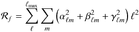 (5)is the regularization functional for the magnetic field. Its role is to prevent the code from introducing high-order modes that are not justified by the observational data. The coefficients Λa and Λf determine the contributions of ℛa and ℛf to the total discrepancy function Ψ. Their values usually are chosen on the basis of a balance between the goodness of the fit and the smoothness of the solution.
Our experiments showed that the value of the appropriate regularization parameter can be found reliably with respect to the value of the other regularization parameter, that is, knowing approximately Λf, we can accurately determine Λa, and vice versa. This claim is easily explained – the abundance distribution strongly affects the Stokes I profiles and depends only slightly on the magnetic field maps for moderately strong magnetic fields, while the Stokes QUV profiles strongly depend on the magnetic field distribution. This translates into the following algorithm: we first calculated the MDI solution on a wide grid of Λa and Λf (in our case the grid was 16 × 16). To determine Λa we considered the change of  with respect to ℛa for a fixed value of Λf. After identifying the optimal value of Λa, we iterated this procedure and assessed the change of
  with respect to ℛf for the previously determined optimal value of Λa, which yields the optimal value for Λf. We iterated once or twice every time with the newly found optimal values of the regularization parameters to ensure that our results were consistent. As a rule, we obtained consistent results after the first iteration.
We experimentally determined the optimal value of each regularization parameter by assessing the change in the corresponding discrepancy function and regularization functional when we decreased it from some starting value that produced a very smooth solution (abundance maps for Λa, and magnetic field maps for Λf). A optimal value was found when an additional decrease of the regularization parameter improved the discrepancy function only weakly and strongly increased the regularization functional (ℛa or ℛf).
3.2. Atmosphere model
Shulyak et al. (2009) constructed a self-consistent model atmosphere for HD 24712 that takes the stratification of chemical elements into account. The authors derived the model atmosphere from iterative fitting of the observed high-resolution spectra and spectral energy distribution data using atmospheric models that account for the effects of individual and stratified abundances. A significant part of their paper is devoted to the non-local thermodynamic equilibrium (NLTE) treatment of the formation of Pr ii/iii and Nd ii/iii lines, which appears to seriously influence the atmosphere structure by creating an inverse temperature gradient caused by the overabundance of rare earth elements (REE) in the upper atmospheric layers.
The detailed, self-consistent analysis of HD 24712 performed by Shulyak et al. (2009) is a good basis for our MDI study. Consequently, we adopted one of their models with stratified abundances, model number four (see Table 3 in their paper), which was calculated for Teff = 7250 K, log g = 4.1, and a scaled REE opacity for Pr ii and Nd ii ions. This model is sufficient for our work because it accurately describes the mean atmosphere and effects of stratification and does not differ significantly from the model with a scaled REE opacity for Pr iii and Nd iii in addition to the opacity for Pr ii and Nd ii ions. The initial abundance values of the elements that we mapped were set to the values measured from the mean spectrum; for iron we used − 5.5 (in log (NX/Ntot) units), for neodymium − 9.0, and − 7.0 for sodium.
We address one final concern that might arise from our use of single mean model atmosphere for the MDI analysis of HD 24712. Kochukhov et al. (2012) investigated this problem for the magnetic Ap star α2 CVn. Their experiments showed that using a grid of model atmospheres that reflect the local surface abundance distribution of the mapped chemical elements only slightly improves the fit to Stokes I, and has practically no effect on the polarization profiles or on the resulting magnetic field and abundance maps. In addition to this, the abundance contrast of the most important elements Fe, Cr, and Si for HD 24712 is much less extreme than that of α2 CVn. Therefore, we proceeded with using a single mean atmosphere model in our study.
3.3. Spectral line selection
Atomic data of spectral lines used for the MDI inversion.
From the available spectropolarimetric observations we selected the 13 Fe i/ii, 3 Nd iii lines and one Na i line. We selected them on the basis of the strong polarization signals in the Stokes QUV profiles, and because of the visible variations with phase in the Stokes I profiles due to abundance inhomogeneities and the Zeeman effect. Spectral lines suffering from significant blending were not included in the line list.
The reason for using these chemical elements is that iron and neodymium have different vertical stratification profiles and the respective Stokes profiles of their spectral lines exhibit different rotational modulation with phase. Moreover, the phase variation of the sodium lines differs from that of the iron and neodymium lines. Therefore, by using these elements, we can fully probe the surface of HD 24712 and obtain a reliable reconstruction of the magnetic field and abundance distribution. A detailed analysis of the behavior of the polarization signatures of individual lines in the spectrum of HD 24712 was presented in Sect. 4 of Paper I.
The complete line list adopted for the MDI inversion of HD 24712 is presented in Table 1. The atomic data for the lines were extracted from the VALD database (Kupka et al. 1999). The Fe i 5434.524 Å line, which is insensitive to the magnetic field, was also included in the line list. This line indicates how well the abundance distribution of iron reproduces the Stokes I profiles of non-magnetic lines. During the inversion procedure we realized that three iron lines had incorrect log gf values. The corrections for these three lines were calculated automatically by the code invers10. The three Nd iii lines were chosen from an initial list of known Nd ii/iii lines on the basis of our criteria. To the oscillator strengths of these lines we added NLTE corrections that were calculated by Mashonkina et al. (2005).
3.4. Optimization of vesin i, Θ, and i
 |
Fig. 1 Variations of the normalized discrepancy function for the Stokes QU profiles, |

Magnetic Doppler imaging in four Stokes parameters in addition to the stellar atmosphere model and the line list requires knowing the orientation of the stellar rotation axis and the projected rotational velocity of the star. The orientation of the stellar rotation axis is determined by the inclination i and azimuth angle Θ. The inclination is defined as the angle between the rotation axis and the line of sight to the observer; it changes from 0° to 180°. The azimuth angle can have values in the range [ 0°,360° ], and it determines the position angle of the sky-projected rotation axis. Note that because the Stokes QU profiles are changing with 2Θ, there is an ambiguity between Θ and Θ + 180°.
The initial values i = 138° and Θ = 29° used here were determined in Paper I, where we combined our longitudinal field and net linear polarization measurements with available broad-band linear polarization data (Leroy 1995) and computed the parameters of the so-called canonical model (Landolfi et al. 1993) for dipolar magnetic field geometry. We adopted 5.6 km s-1 (Ryabchikova et al. 1997) as the initial value for the projected rotational velocity.
Using numerical experiments, Kochukhov & Piskunov (2002) showed that incorrect values of these parameters lead to higher values of the discrepancy function. The optimal value of the rotational velocity can be determined by comparing the discrepancy function for the Stokes I profiles calculated with various values of vesini. Incorrect values of i and Θ lead to a similar increase of the discrepancy function for Stokes Q and U profiles.
To optimize i and Θ we computed 42 MDI solutions on a grid i ∈ [ 100°,160° ] and Θ ∈ [ 5°,55° ] with 10° steps for both angles. The resulting normalized discrepancy function as a function of i and Θ is plotted in Fig. 1. The minimum of the discrepancy function was found for i = 120° and Θ = 35°. We compared the Stokes QU profiles for the optimal values of i and Θ with the values computed for values greater or smaller by 10°, which is the grid step in our case. The comparison showed that with the new values of i and Θ, our MDI procedure appears to better reproduce the observed Stokes QU profiles. We adopted the newly found values of i and Θ as final for the remainder of the paper.
The rotational velocity was determined in a similar matter. We produced 37 individual MDI solutions for vesini in the range of 2 km s-1 to 9 km s-1. We computed the discrepancy function for the Stokes I profiles separately for the Fe, and for the Nd lines. This is necessary because Nd lines require additional broadening for the Stokes I profiles, which is not present in the Fe lines. This phenomenon is known to exist for other Ap stars (see Ryabchikova et al. 2007). In Fig. 2 we illustrate the normalized discrepancy function for Stokes I profiles of the Fe and Nd lines accordingly. From this figure it can be seen that the discrepancy function for the Fe lines is complex, with two close minima in the 5–6 km s-1 range with a peak around 5.5 km s-1. This behavior of the discrepancy function for the Fe lines indicates that we cannot with confidence find optimized vesini. We also point out the significantly higher vesini ≃ 7.1 km s-1 derived from Nd lines. Although they are less sensitive to changes in vesini, the discrepancy functions for the remaining Stokes parameters can be used in a similar manner to understand the range where vesini is the most probable. The discrepancy functions for these Stokes parameters showed clearly defined minima in the range 5–6 km s-1. As a result, we decided to adopt a new value for vesini = 5.5 ± 0.5 km s-1 corresponding to the center of that range. In the remaining paper this value of vesini is used for all other MDI inversions.
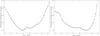 |
Fig. 2 Normalized discrepancy function |
4. Results
4.1. Individual vs. simultaneous MDI of chemical elements
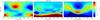 |
Fig. 3 Differences in the abundance distribution of Fe, Nd iii, and Na from their individual mapping relative to the corresponding maps from the simultaneous MDI of these elements. We note that for Na mapping we used the magnetic field maps derived from the simultaneous MDI inversion of the Fe and Nd iii lines. In each panel we mark the 16 and 84 percentiles with white and black lines. The bar on the right indicates the abundance difference in log (NX/Ntot) units of element X. |
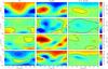 |
Fig. 4 Differences in distribution of the magnetic field components relative to the corresponding maps from the simultaneous MDI of Fe, Nd iii and Na. In rows one to four we plot the differences for the radial, meridional, and azimuthal components of the magnetic field and for the field modulus. In Col. 1 we plot the differences for the magnetic field components derived from the MDI inversion of Fe; in Col. 2 we plot the same quantities for Nd iii; in Col. 3 we plot the differences of the magnetic field components derived from the simultaneous MDI of Fe and Nd iii lines. In each plot we mark the 16 and 84 percentiles with white and black lines. The bars on the right indicate the difference of the corresponding components measured in kG. |
Our magnetic Doppler imaging study was separated into three steps. The first step involved producing maps of the magnetic field and chemical abundance from individual mapping of Fe and Nd iii. In the second step we produced magnetic field and abundance distribution maps from simultaneous mapping of Fe and Nd iii. Additionally, we used the magnetic field maps produced in this step and calculated abundance map for Na. In the third step we performed simultaneous MDI mapping of the three chemical elements Fe, Nd iii, and Na. The magnetic field and abundance distribution maps calculated in the third step are called the final maps.
In this section we investigate how reliable the results are that were produced from individual versus simultaneous MDI of Fe, Nd iii, and Na. Ideally, all maps, whether they are produced from individual or simultaneous mapping of chemical elements, should show the same results. However, as a result of the inhomogeneous surface distribution of the chemical elements in the atmospheres of Ap stars, spectral lines of different elements can be sensitive to certain parts of the surface of the star by a different amount. Therefore, it is necessary to have a line list that probes the entire stellar surface and not just parts of it. Our line list, discussed in Sect. 3.3, is the result of this argument. We note that while the MDI analysis for Fe and Nd iii in steps one and two was self-consistent, meaning that we derived abundance and magnetic field maps, for the single Na line we used the already derived magnetic field maps from simultaneous MDI of Fe and Nd iii. In this way, we can test how the single Na line affects our final results. The reasoning behind this is that mapping the magnetic field and abundance distribution from one single line can give biased results. Additionally, our Na line cannot be fitted satisfactorily by the code invers10, which might raise questions about the quality and reliability of our inversions.
We compared two maps M1 and M2 calculated on the same surface grid by calculating the difference, M1 − M2, from which we computed the median value, and 16 and 84 percentiles that for a normal distribution are the same as one standard deviation below and above the mean value. We preferred using the 16 and 84 percentiles and the median instead of the classical statistical estimators – the mean and standard deviation – to minimize possible effects of long non-normal tails that are sometimes present in MDI maps.
We also compared the morphological features of the two maps by eye. For the magnetic field maps we also assessed the relative energy of their poloidal and toroidal components as a function of spherical harmonics number ℓ (see Sect. 3.1). We did this to compare the magnetic field geometry of different solutions.
The differences of abundance distribution maps of Fe, Nd iii, and Na relative to the corresponding final maps can be found in Fig. 3. The analogous quantities for the magnetic field maps derived from individual mapping of Fe and Nd iii relative to the respective final magnetic field maps are presented in Fig. 4. Figure 5 compares the energies of the poloidal and toroidal harmonic modes.
We now consider the resulting difference maps for the abundance distribution of the mapped chemical elements. The differences in the distribution of Fe derived from individual mapping relative to its final map agree well. The difference map has median value of − 0.02 dex and shows no statistically significant systematic shifts relative to the final map. Furthermore, the morphological properties of the two Fe maps show no significant differences – the two recovered maps have similar features.
The Nd iii difference map agrees similarly well, with a median value of − 0.07 dex. One almost circular area around the visible magnetic pole with approximately 0.5 dex overabundance relative to the final Nd iii map deserves closer consideration. Taking into account its relatively small surface area and the large effective abundance range of the final map of 2.6 dex, we suggest that this spot only weakly influences the final results.
Finally, the abundance map produced for Na shows no systematic shifts from the final Na map with median value of − 0.05 dex. Although in this case, the difference map shows that the individual map deviates more strongly from the final map, about 0.3 dex, this is still much smaller than the effective abundance range of 3.5 dex for the final map. Thus, we consider the Na map to be reproduced reliably.
The difference maps for the magnetic field are more complicated. For Fe the recovered magnetic field tends to be weaker by about 0.22 kG, as given by the median value of the difference for the field modulus. This is especially noticeable in Fig. 4 (row 4, Col. 1). Despite the weaker field strength, 94.5% of the energy of the field is located in the first harmonic of the poloidal field component (Fig. 5, panel 1). This indicates that by using only Fe lines for the derivation of the magnetic field maps of HD 24712, we risk obtaining a weaker field.
The difference maps of the magnetic field derived from Nd iii lines vary by about 0.35 kG for all components of the field. Despite this, the energy of the magnetic field derived from the individual mapping of Nd iii is almost identical to the energy from Fe. The strongest component is the poloidal one for the first harmonic with 97% of the total magnetic field energy (Fig. 5, panel 2) versus 96% for the same component in the final map.
Finally, the magnetic field maps derived from simultaneous MDI of Fe and Nd iii deviate very little (<0.15 kG) from the appropriate final maps. Therefore, adding the single Na line to our line list does not significantly change our final maps.
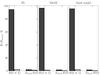 |
Fig. 5 Relative energies of the poloidal and toroidal harmonic modes for the magnetic field topology of HD 24712. In panels one to three we show the relative energies of the magnetic field from individual MDI of Fe, Nd iii, and from simultaneous MDI of Fe, Nd iii, and Na (final model). The energy of the poloidal and toroidal modes in each panel are shown in dark and light gray. The first bar in each panel for the corresponding energy mode (poloidal, toroidal) is for ℓ = 1; the second such bar represents the sum for all energies with ℓ ≥ 2. |
In summary, we conclude the following:
-
1.
The abundance maps of Fe, Nd, and Na computed from theirindividual inversions have the same morphology and show nosignificant systematic shifts compared with the correspondingfinal maps computed from simultaneousMDI inversion. The discrepancy between therespective maps is about 0.15 dex for Fe and Nd,and lower than 0.3 dex for Na.
-
2.
We constrained the different components of the magnetic field of HD 24712 with an accuracy of approximately 0.3 kG.
-
3.
Using single elements in MDI inversions can lead to a systematic bias of the reconstructed magnetic field. Our analysis for the example of HD 24712 emphasizes that a proper MDI study of Ap stars needs to be performed with a set of lines that probes the entire surface of the star.
-
4.
The energy of the magnetic field as a function of the spherical harmonic degree ℓ changes by about 1%, whether derived from individual or simultaneous MDI inversion of Fe and Nd, which implies that the global magnetic field geometry of HD 24712 is constrained reliably in both cases.
4.2. Maps from simultaneous MDI of Fe, Nd III, and Na
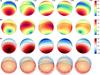 |
Fig. 6 Distribution of the magnetic field on the surface of HD 24712 derived from simultaneous MDI analysis of Fe, Nd iii, and Na. The plots show the distribution of magnetic field modulus (first row), horizontal field (second row), radial field (third row), and field orientation (fourth row) on the surface of HD 24712. The bars on the right indicate the field strength in kG. The contours are plotted in steps of 1 kG. The arrow length in the bottom plot is proportional to the field strength. The star is shown at five rotational phases, indicated above the spherical plots. |
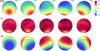 |
Fig. 7 Abundance distribution of Nd iii, Fe, and Na on the surface of HD 24712. The first row shows the surface map of the Nd iii, the second and third rows illustrate the surface abundance maps of Fe and Na. These maps were derived from the simultaneous mapping of the three elements. The bars on the right next to each panel indicate the abundance in log (NX/Ntot) units of element X. The contours are plotted with a step of 0.4 dex Nd iii and Na, and 0.2 dex for Fe. The vertical bar indicates the rotation axis. |
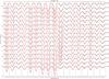 |
Fig. 8 Comparison of the observed (dots connected with lines) and synthetic (lines) Stokes I profiles calculated for the final magnetic field and abundance maps (Figs. 7 and 6) for all lines used in the MDI inversion. The distance between two consecutive ticks on the horizontal top axis of each panel is 0.1 Å, indicating the wavelength scale. Rotational phases are indicated on the right of the figure. |
The final magnetic field and abundance maps derived from the simultaneous mapping of Fe, Nd iii, and Na are shown in Figs. 6 and 7. In Fig. 6 we plot the spherical projection of the field modulus  , the strength of the horizontal
  and radial field Br components; the bottom row shows the vector magnetic field. The comparison of the observed and the calculated line profiles for the entire line selection is presented in Figs. 8–11.
The reconstructed magnetic field of HD 24712 appears to be mostly poloidal and dipole-like. The poloidal harmonic component with ℓ = 1 dominates all other toroidal and poloidal harmonics, containing 96% of the total magnetic field energy. The contribution of all other modes with  is much less significant, as shown in Fig. 5 (panel 3).
There is a slight asymmetry between the positive (visible) and negative magnetic pole in our final magnetic field maps, see Fig. 6, by approximately 0.6 kG. This discrepancy probably does not represent sufficient evidence that the magnetic field topology of HD 24712 deviates strongly from axial symmetry. It might be caused purely by the nature of the magnetic field configuration of the star, where only the positive magnetic pole is visible by an observer from Earth.
We conclude that the magnetic field topology of HD 24712 has a dominant dipolar component with a very weak contribution at smaller spatial scales from higher-order harmonics. This result contrasts with the finding of a roughly dipole-like global field with strong small-scale features for α2 CVn (Kochukhov & Wade 2010) and with the quasi-dipolar field of 53 Cam, which has a mostly dipolar poloidal component with toroidal contributions of similar strength on spatial scales of 30°–40° (Kochukhov et al. 2004b).
The abundance distribution of Fe and Nd iii for HD 24712 was previously derived by Lüftinger et al. (2010) from an MDI study of Fe and Nd iii lines using only Stokes I and V parameters. The new maps confirm these findings and also show some details the previous study lacked.
The abundance distribution of Fe varies between − 5.53 and − 4.86 dex on the log (NX/Ntotal) scale. One new detail is the appearance of a roughly circular area around the positive magnetic pole that is strongly depleted relative to the median value by about 0.3 dex. The new Nd iii abundance map shows significantly stronger variations that change from − 8.66 to − 6.04 dex. This corresponds to a range of values of 2.61 dex versus the 1.1 dex reported by Lüftinger et al. (2010). The range of the abundance values for Fe is 0.67 dex and matches the range reported in the previous study.
We also found a discrepancy in the location of the Nd spot. Lüftinger et al. (2010) detected a possible longitudinal offset, amounting to 0.04 of the rotation period, of the position of the maximum of the Nd iii abundance map relative to the maximum of the magnetic field. Our MDI study shows that the longitudinal offset for Nd iii is very small, if present at all. We attribute this to the better quality of our observational material and the denser phase sampling, resulting in a higher accuracy when determining longitudinal position of abundance spots; Lüftinger et al. (2010) could determine longitudinal positions of abundance structures with a precision of 0.02–0.05 rotational periods. We also found that our adopted period, which is slightly shorter than the period used by Lüftinger et al. (2010), results in a positive longitudinal shift of about 0.01 rotational periods relative to the previous study. Therefore, the lack of a visible longitudinal offset of the maximum of the Nd iii abundance map relative to the position of the maximum of the magnetic field in this work might be caused by a combination of the higher quality of the observations and the revised rotational period used here.
The abundance distribution maps of Fe and Nd iii (Fig. 7) in combination with the magnetic field maps (Fig. 6) reproduce the Stokes profiles of the spectral lines reasonably well. However, there are certain discrepancies in minor spectral details. This can be seen in the Stokes I line profiles of Fe i 6336.824 Å. This line has a simple Zeeman-splitting pattern and is highly sensitive to the magnetic field, which results in the appearance of two partially resolved components that are easily visible in the observed Stokes I profiles (Fig. 8), but the synthetic line profiles do not show this splitting. The second example with a similar behavior is the Fe ii 6432.68 Å line, for which the code invers10 does not produce the characteristic splitting in the Stokes I profiles either.
Another discrepant behavior is observed in the Stokes Q profiles of the Nd iii lines, for which the code invers10 cannot reproduce the blue wing of the profiles around the maximum of the magnetic field. This problem persists even for an MDI inversion using only Nd iii lines, although the discrepancy is less pronounced.
These discrepancies probably do not affect our results significantly. For the Fe lines with visible Zeeman splitting in the Stokes I profiles, their general behavior with phase is reproduced on a satisfactory level. The observed behavior in the calculated Stokes Q profiles of the Nd iii lines can be caused by the Stokes Q profiles of Fe lines, which are systematically weaker and more numerous than Nd iii line profiles (13 versus 3) and thus contribute more to the MDI solution.
For the first time for HD 24712, we here attempted to derive an abundance map of Na. The resulting abundance map explains the behavior of Na lines fairly well, whose profiles change in anti-phase to Nd lines. The abundance map of this element shows a strong horizontal gradient, its range of values is 3.49 dex and changes from − 8.65 to − 5.16 dex. The morphological characteristics of the Na abundance map contrasts with the map for Nd iii; Na is overabundant near the negative magnetic pole, which is invisible to the observer from Earth, and is depleted near the positive magnetic pole. This abundance distribution of Na explains the peculiar behavior of the circular polarization profile of the Na i 5889.951 Å line, which changes sign around zero phase. However, special care has to be taken when interpreting these results. In Figs. 8–11 we see that our best fit for this line does not properly describe its behavior around zero phase corresponding to magnetic maximum. Our further analysis of this line showed that to fully reproduce the behavior of the line profiles of Na i 5889.951 Å with phase, we need to allow the code invers10 to produce an abundance map with a range of values of 5.6 dex instead of with the 3.5 dex for the map presented in Fig. 7. For such an abundance map the regularization parameter Λa is non-optimal (see Sect. 3.1).
We suspect that the reason for the insufficiently good fit of the Na i line might be the strong vertical stratification that is made even more complex by NLTE effects. In our current version of the code invers10 we do not account for these effects. We plan to investigate vertical stratification structures in a future paper.
4.3. Dipolar field parameters
In Paper I we considered our longitudinal magnetic field and net linear polarization measurements inferred from the LSD profiles of HD 24712 together with available broad-band linear polarization measurements obtained by Leroy (1995) in the framework of the so-called canonical model introduced by Landolfi et al. (1993), and derived the global magnetic field parameters for a purely dipolar magnetic field geometry. The global field parameters agreed well with the previous result obtained by Bagnulo et al. (1995), with the exception of a somewhat lower Bp obtained by us.
Because in this work we used a spherical harmonics decomposition of the magnetic field, it is possible to use the coefficients of the decomposition that correspond to the poloidal field for ℓ = 1 to derive the dipole field strength Bp and the angle β between the rotation axis and the magnetic axis. Using this approach, we derived Bp = 3439 G and β = 160° from the solution that was computed from the simultaneous mapping of Fe, Nd iii, and Na.
The comparison of the newly derived values for the dipolar magnetic field parameters with the values presented in Paper I shows that the new value for Bp is within three sigma of the previous measurement; the slightly higher value of β by about 15° relative to its previous value may be related to the revised value for the inclination angle i = 120° we adopted here (see Sect. 3.4).
We emphasize that the values for Bp and β were derived using only a subset of the spherical harmonics coefficients derived in our study and therefore represent a simplified picture of the magnetic field of HD 24712.
4.4. Stokes profiles and surface distribution of calcium
 |
Fig. 12 Abundance distribution of Ca on the surface of HD 24712. The bar on the far right denotes the abundance in log (NCa/Ntot) units. The contours are plotted with steps of 0.4 dex. The vertical bar in each projection indicates the rotation axis. Phase is indicated in the upper right corner of each projection. |
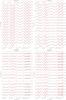 |
Fig. 13 Comparison of the observed (dots connected with lines) and synthetic (lines) Stokes profiles for Ca calculated for the final magnetic field (Fig. 6) and abundance distribution (Fig. 12). The distance between two consecutive ticks on the horizontal top axis of each panel is 0.1 Å, indicating the wavelength scale. Rotational phases are indicated on the right of each panel. |
Lüftinger et al. (2010) attempted to use their magnetic field maps to derive abundance distribution of Ca, but because of limitations of the observational data, they were unable to derive results of any significance. Our unique observational data set opens new possibilities of investigating the abundance distribution for Ca.
This element was studied by Ryabchikova et al. (1997) and was used by Shulyak et al. (2009) for their vertical stratification analysis, which showed that Ca has a vertical stratification profile similar to that of Fe. It is of particular interest to see how our magnetic field maps reproduce the spectral features of a chemical element with previously unknown abundance distribution. The Ca lines of HD 24712 are well suited for this purpose.
The line list of Ca lines, shown in Table 2, was composed on basis of the same principles as discussed in Sect. 3.3 – the Ca lines were selected based on their phase variations, polarization signatures, and lack of blending by other spectral lines.
Atomic data of spectral lines used for the MDI inversion of calcium.
We used the magnetic field maps (Fig. 6) from the simultaneous MDI study of Fe, Nd iii, and Na as fixed parameters and derived abundance distribution of Ca. The resulting map for Ca is shown in Fig. 12. The computed and observed Ca line profiles are compared in Fig. 13, which shows that most polarization signatures in the Stokes QUV profiles are reproduced satisfactorily. There are some exceptions in the Stokes I profiles for several lines, in particular for Ca i 6162.173 Å and Ca i 5857.451 Å. This might be caused by an inhomogeneous vertical distribution of Ca in the atmosphere of HD 24712.
The abundance map of Ca varies across the stellar surface between − 5.4 dex and − 7.1 dex. Interestingly, Ca shows an overabundance area close to the magnetic equator and a roughly circular patch at the visible magnetic pole where Ca is depleted relative to its median value. From the comparison of Figs. 7 and 12 we see that this coincides with the abundance map of Fe, which has a similar circular patch around the visible magnetic pole, where Fe is underabundant. One should be careful when interpreting these results because some Ca and Fe lines can be influenced by vertical stratification. It is possible that the roughly circular underabundance patches at the location of the visible magnetic pole derived in our MDI inversions are an artifact caused by ignoring vertical stratification.
5. Discussion
5.1. Theoretical interpretation of the magnetic field in HD 24712
The discovery of the dipole-like, axisymmetric magnetic field for HD 24712 from our MDI study of four Stokes parameter observations provides a new perspective on the question of the origin and stability of magnetic fields in intermediate-mass main sequence A and late B stars. The general idea behind the existence of magnetic fields in these stars is the so-called fossil field hypothesis, which postulates that the magnetic fields of these stars are remnants from an earlier evolutionary phase. This hypothesis is supported by the long-term stability and large-scale nature of these magnetic fields coupled with the wide range of field strengths observed. One of the challenges of this theory was to find stable magnetic field equilibrium configurations that can be present in stellar interiors. Recent theoretical advances (Braithwaite & Nordlund 2006; Braithwaite 2008, 2009) have shown that stable magnetic fields can exist in the interiors of these stars. Braithwaite & Nordlund (2006) and Braithwaite (2008) found that for a stable, stratified star with initial random magnetic field configuration, the magnetic field evolves on Alfveń time-scales (tens of years for the typical Ap stars) into a stable equilibrium configuration of twisted flux tubes.
These equilibrium configurations appear to depend on the initial conditions (Braithwaite 2009), which may explain the wide variety of magnetic field configurations inferred from MDI studies. There are roughly two characteristic stable configurations – an approximately axisymmetric equilibrium with one flux tube forming a circle around the equator, and a non-axisymmetric equilibrium solution with one or more flux tubes arranged in a more complex pattern. The axisymmetric configuration in observations presents itself roughly as a dipole, with smaller contributions from higher multipoles. In contrast to this, the non-axisymmetric equilibrium configurations result in highly complex magnetic field geometries such as those found for τ Sco (Donati et al. 2006) and HD 37776 (Kochukhov et al. 2011).
An interesting conjecture proposed by Braithwaite & Nordlund (2006) is that Ap stars with almost exact dipole fields are older than Ap stars with more structure on smaller scales. This conjecture can be verified only by MDI studies based on four Stokes parameter observations.
At this stage, only two stars in addition to HD 24712 have been investigated with the MDI technique using all Stokes parameters. Kochukhov & Wade (2010) studied α2 CVn and found dipole-like magnetic field with small-scale features, which have much higher field strength than in the surrounding areas. The second object is 53 Cam, for which Kochukhov et al. (2004a) showed that a quasi-dipolar magnetic field with strong toroidal components at angular scales of 30°–40° is necessary to fit the available spectropolarimetric observations.
For the purpose of this analysis we used the stellar ages of our objects published by Kochukhov & Bagnulo (2006); 9.07 for HD 24712, 8.27 for α2 CVn, and 8.84 for 53 Cam. The values adopted here are in log t (yr) units.
Given these results, our finding of the dipole-like, axisymmetric magnetic field for HD 24712, which is the oldest star in our three star sample, gives some evidence for the hypothesis that old Ap stars have predominantly dipolar magnetic fields with little structure on small scales.
Our future plans involve performing MDI in four Stokes parameters of other Ap/Bp stars with different masses and ages, which will help us further assess this hypothesis and investigate the dependence of the magnetic field geometry on other stellar parameters.
5.2. Abundance distribution of chemical elements and atomic diffusion
The patchy abundance distribution and vertical stratification of chemical elements in the atmospheres of Ap stars is thought to be caused by atomic diffusion in the presence of a magnetic field (Michaud et al. 1981; LeBlanc et al. 2009; Alecian & Stift 2010). According to this model, some elements are expected to accumulate and form cloud-like structures in the atmospheres of Ap stars. However, theoretical predictions arising from this theory have in general been only qualitative in the case of magnetic Ap stars, with little predictive power for individual stars.
We compared our empirical abundance maps from the latest MDI analysis of HD 24712 with the theoretical results of Alecian & Stift (2010), who computed a 2D stratification for a number of elements for several values of effective temperature and dipole field strength. These authors deduced the appearance of narrow belts of enhanced metals around the magnetic equator for stars with a dipole magnetic field. For stars with a non-dipolar field, the abundance patches would be created at places where the field lines are parallel to the local surface. The abundance maps for Fe, Nd, and Na derived in this study do not show such abundance structures. Instead, the Fe and Ca abundance maps very roughly correlate with the field modulus (compare Figs. 7 and 12 with Fig. 6 for Fe and Ca). The abundance maps for Nd and Na anti-correlate and show strong abundance gradients between the two polar regions. Alecian & Stift (2010) suggested that such a large abundance difference between the polar regions might be caused by a non-dipolar configuration or by a decentered dipole with significant difference in field strength at the poles. It appears that our results from MDI inversion using four Stokes vector observations of HD 24712 refute this suggestion, because the newly derived magnetic field is dipole-like to a very high extent, and although the magnetic field maps do indeed show a slight asymmetry of approximately 0.6 kG between the poles, we do not consider this to be a “significant” difference in strength.
We conclude that our abundance maps of Fe, Nd, Na, and Ca do not show behavior consistent with the presence of a narrow overabundance belt around the magnetic equator. Better theoretical models are required to explain the variety of the observed abundance distributions of chemical elements in the atmosphere of HD 24712.
6. Conclusions
We presented results of the MDI study of the cool Ap star HD 24712. This is the first such analysis for a rapidly oscillating Ap star performed on the basis of phase-resolved spectropolarimetric observations of line profiles in all four Stokes parameters that have a resolving power exceeding 105 and a signal-to-noise ratio of 300–600.
The main results from our investigation are summarized below.
-
The magnetic field topology of HD 24712 ismostly poloidal and dipolar, with small contributions fromhigher order harmonics. We found a small differencebetween the positive and negative magnetic pole of approximately 0.6 kG in field modulus. This can be attributed to the nature of the magnetic fieldconfiguration of HD 24712, for which onlythe positive magnetic pole is visible by an observer fromEarth.
-
The recovered abundance distribution map of Fe shows enhancements on both sides of the magnetic equator. The abundance map of Ca shows enhancements only on the side of the magnetic equator with the positive magnetic pole. Both maps show an underabundance patch centered on the visible magnetic pole. The polar feature may represent an artifact caused by ignoring vertical chemical stratification of Fe and Ca in the atmosphere of HD 24712.
-
The recovered abundance maps of Nd and Na show a strong anti-correlation. Nd is highly abundant around the visible magnetic pole, while Na is overabundant around the negative magnetic pole.
-
We found tentative evidence for the hypothesis that Ap stars with dipole-like fields that have weak contribution from higher-order harmonics are older or less-massive than stars with magnetic fields that have more small-scale structures.
-
The derived abundance maps of Fe, Nd, Na, and Ca are inconsistent with current theoretical predictions of atomic diffusion theory in the presence of magnetic fields.
Acknowledgments
O.K. is a Royal Swedish Academy of Sciences Research Fellow, supported by grants from the Knut and Alice Wallenberg Foundation and Swedish Research Council. The computations were performed on resources provided by SNIC through Uppsala Multidisciplinary Center for Advanced Computational Science (UPPMAX) under project snic2013-11-24. T.R. acknowledges partial financial support from the Presidium RAS Program “Nonstationary Phenomena in Objects of the Universe”. Resources provided by the electronic databases (VALD, Simbad, NASA ADS) are gratefully acknowledged.
References
- Alecian, G., & Stift, M. J. 2010, A&A, 516, A53 [NASA ADS] [CrossRef] [EDP Sciences] [Google Scholar]
- Bagnulo, S., Landi Degl’Innocenti, E., Landolfi, M., & Leroy, J. L. 1995, A&A, 295, 459 [NASA ADS] [Google Scholar]
- Bagnulo, S., Wade, G. A., Donati, J.-F., et al. 2001, A&A, 369, 889 [NASA ADS] [CrossRef] [EDP Sciences] [Google Scholar]
- Braithwaite, J. 2008, MNRAS, 386, 1947 [NASA ADS] [CrossRef] [Google Scholar]
- Braithwaite, J. 2009, MNRAS, 397, 763 [NASA ADS] [CrossRef] [Google Scholar]
- Braithwaite, J., & Nordlund, Å. 2006, A&A, 450, 1077 [NASA ADS] [CrossRef] [EDP Sciences] [Google Scholar]
- Donati, J.-F., & Brown, S. F. 1997, A&A, 326, 1135 [NASA ADS] [Google Scholar]
- Donati, J.-F., Howarth, I. D., Jardine, M. M., et al. 2006, MNRAS, 370, 629 [NASA ADS] [CrossRef] [Google Scholar]
- Kochukhov, O., & Bagnulo, S. 2006, A&A, 450, 763 [NASA ADS] [CrossRef] [EDP Sciences] [Google Scholar]
- Kochukhov, O., & Piskunov, N. 2002, A&A, 388, 868 [NASA ADS] [CrossRef] [EDP Sciences] [Google Scholar]
- Kochukhov, O., & Wade, G. A. 2010, A&A, 513, A13 [NASA ADS] [CrossRef] [EDP Sciences] [Google Scholar]
- Kochukhov, O., Bagnulo, S., Wade, G. A., et al. 2004a, A&A, 414, 613 [NASA ADS] [CrossRef] [EDP Sciences] [Google Scholar]
- Kochukhov, O., Ryabchikova, T., & Piskunov, N. 2004b, A&A, 415, L13 [NASA ADS] [CrossRef] [EDP Sciences] [Google Scholar]
- Kochukhov, O., Lundin, A., Romanyuk, I., & Kudryavtsev, D. 2011, ApJ, 726, 24 [Google Scholar]
- Kochukhov, O., Wade, G. A., & Shulyak, D. 2012, MNRAS, 421, 3004 [NASA ADS] [CrossRef] [Google Scholar]
- Kochukhov, O., Lüftinger, T., Neiner, C., Alecian, E., & MiMeS Collaboration 2014, A&A, 565, A83 [NASA ADS] [CrossRef] [EDP Sciences] [Google Scholar]
- Kupka, F., Piskunov, N., Ryabchikova, T. A., Stempels, H. C., & Weiss, W. W. 1999, A&AS, 138, 119 [NASA ADS] [CrossRef] [EDP Sciences] [MathSciNet] [PubMed] [Google Scholar]
- Landolfi, M., Landi Degl’Innocenti, E., Landi Degl’Innocenti, M., & Leroy, J. L. 1993, A&A, 272, 285 [NASA ADS] [Google Scholar]
- Landstreet, J. D., & Mathys, G. 2000, A&A, 359, 213 [NASA ADS] [Google Scholar]
- LeBlanc, F., Monin, D., Hui-Bon-Hoa, A., & Hauschildt, P. H. 2009, A&A, 495, 937 [NASA ADS] [CrossRef] [EDP Sciences] [Google Scholar]
- Leroy, J. L. 1995, A&AS, 114, 79 [NASA ADS] [Google Scholar]
- Lüftinger, T., Kochukhov, O., Ryabchikova, T., et al. 2010, A&A, 509, A71 [NASA ADS] [CrossRef] [EDP Sciences] [Google Scholar]
- Mashonkina, L., Ryabchikova, T., & Ryabtsev, A. 2005, A&A, 441, 309 [NASA ADS] [CrossRef] [EDP Sciences] [Google Scholar]
- Mathys, G. 1988, A&A, 189, 179 [NASA ADS] [Google Scholar]
- Mathys, G., & Hubrig, S. 1997, A&AS, 124, 475 [NASA ADS] [CrossRef] [EDP Sciences] [Google Scholar]
- Mayor, M., Pepe, F., Queloz, D., et al. 2003, The Messenger, 114, 20 [NASA ADS] [Google Scholar]
- Michaud, G., Charland, Y., & Megessier, C. 1981, A&A, 103, 244 [NASA ADS] [Google Scholar]
- Piskunov, N., & Kochukhov, O. 2002, A&A, 381, 736 [NASA ADS] [CrossRef] [EDP Sciences] [Google Scholar]
- Piskunov, N., Snik, F., Dolgopolov, A., et al. 2011, The Messenger, 143, 7 [NASA ADS] [Google Scholar]
- Rusomarov, N., Kochukhov, O., Piskunov, N., et al. 2013, A&A, 558, A8 [NASA ADS] [CrossRef] [EDP Sciences] [Google Scholar]
- Ryabchikova, T. A., Landstreet, J. D., Gelbmann, M. J., et al. 1997, A&A, 327, 1137 [NASA ADS] [Google Scholar]
- Ryabchikova, T., Sachkov, M., Kochukhov, O., & Lyashko, D. 2007, A&A, 473, 907 [NASA ADS] [CrossRef] [EDP Sciences] [Google Scholar]
- Shulyak, D., Ryabchikova, T., Mashonkina, L., & Kochukhov, O. 2009, A&A, 499, 879 [NASA ADS] [CrossRef] [EDP Sciences] [Google Scholar]
- Silvester, J., Wade, G. A., Kochukhov, O., et al. 2012, MNRAS, 426, 1003 [NASA ADS] [CrossRef] [Google Scholar]
- Silvester, J., Kochukhov, O., & Wade, G. A. 2014, MNRAS, 440, 182 [NASA ADS] [CrossRef] [Google Scholar]
- Snik, F., Kochukhov, O., Piskunov, N., et al. 2011, in Solar Polarization 6, eds. J. R. Kuhn, D. M. Harrington, H. Lin, et al., ASP Conf. Ser., 437, 237 [Google Scholar]
- Stibbs, D. W. N. 1950, MNRAS, 110, 395 [NASA ADS] [CrossRef] [Google Scholar]
- Wade, G. A., Donati, J.-F., Landstreet, J. D., & Shorlin, S. L. S. 2000, MNRAS, 313, 823 [NASA ADS] [CrossRef] [MathSciNet] [Google Scholar]
All Tables
All Figures
|
Fig. 1 Variations of the normalized discrepancy function for the Stokes QU profiles, |
| In the text | |
|
Fig. 2 Normalized discrepancy function |
| In the text | |
|
Fig. 3 Differences in the abundance distribution of Fe, Nd iii, and Na from their individual mapping relative to the corresponding maps from the simultaneous MDI of these elements. We note that for Na mapping we used the magnetic field maps derived from the simultaneous MDI inversion of the Fe and Nd iii lines. In each panel we mark the 16 and 84 percentiles with white and black lines. The bar on the right indicates the abundance difference in log (NX/Ntot) units of element X. |
| In the text | |
|
Fig. 4 Differences in distribution of the magnetic field components relative to the corresponding maps from the simultaneous MDI of Fe, Nd iii and Na. In rows one to four we plot the differences for the radial, meridional, and azimuthal components of the magnetic field and for the field modulus. In Col. 1 we plot the differences for the magnetic field components derived from the MDI inversion of Fe; in Col. 2 we plot the same quantities for Nd iii; in Col. 3 we plot the differences of the magnetic field components derived from the simultaneous MDI of Fe and Nd iii lines. In each plot we mark the 16 and 84 percentiles with white and black lines. The bars on the right indicate the difference of the corresponding components measured in kG. |
| In the text | |
|
Fig. 5 Relative energies of the poloidal and toroidal harmonic modes for the magnetic field topology of HD 24712. In panels one to three we show the relative energies of the magnetic field from individual MDI of Fe, Nd iii, and from simultaneous MDI of Fe, Nd iii, and Na (final model). The energy of the poloidal and toroidal modes in each panel are shown in dark and light gray. The first bar in each panel for the corresponding energy mode (poloidal, toroidal) is for ℓ = 1; the second such bar represents the sum for all energies with ℓ ≥ 2. |
| In the text | |
|
Fig. 6 Distribution of the magnetic field on the surface of HD 24712 derived from simultaneous MDI analysis of Fe, Nd iii, and Na. The plots show the distribution of magnetic field modulus (first row), horizontal field (second row), radial field (third row), and field orientation (fourth row) on the surface of HD 24712. The bars on the right indicate the field strength in kG. The contours are plotted in steps of 1 kG. The arrow length in the bottom plot is proportional to the field strength. The star is shown at five rotational phases, indicated above the spherical plots. |
| In the text | |
|
Fig. 7 Abundance distribution of Nd iii, Fe, and Na on the surface of HD 24712. The first row shows the surface map of the Nd iii, the second and third rows illustrate the surface abundance maps of Fe and Na. These maps were derived from the simultaneous mapping of the three elements. The bars on the right next to each panel indicate the abundance in log (NX/Ntot) units of element X. The contours are plotted with a step of 0.4 dex Nd iii and Na, and 0.2 dex for Fe. The vertical bar indicates the rotation axis. |
| In the text | |
|
Fig. 8 Comparison of the observed (dots connected with lines) and synthetic (lines) Stokes I profiles calculated for the final magnetic field and abundance maps (Figs. 7 and 6) for all lines used in the MDI inversion. The distance between two consecutive ticks on the horizontal top axis of each panel is 0.1 Å, indicating the wavelength scale. Rotational phases are indicated on the right of the figure. |
| In the text | |
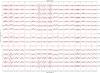 |
Fig. 9 Same as Fig. 8 for the Stokes Q profiles. |
| In the text | |
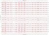 |
Fig. 10 Same as Fig. 8 for the Stokes U profiles. |
| In the text | |
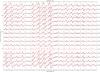 |
Fig. 11 Same as Fig. 8 for the Stokes V profiles. |
| In the text | |
|
Fig. 12 Abundance distribution of Ca on the surface of HD 24712. The bar on the far right denotes the abundance in log (NCa/Ntot) units. The contours are plotted with steps of 0.4 dex. The vertical bar in each projection indicates the rotation axis. Phase is indicated in the upper right corner of each projection. |
| In the text | |
|
Fig. 13 Comparison of the observed (dots connected with lines) and synthetic (lines) Stokes profiles for Ca calculated for the final magnetic field (Fig. 6) and abundance distribution (Fig. 12). The distance between two consecutive ticks on the horizontal top axis of each panel is 0.1 Å, indicating the wavelength scale. Rotational phases are indicated on the right of each panel. |
| In the text | |
Current usage metrics show cumulative count of Article Views (full-text article views including HTML views, PDF and ePub downloads, according to the available data) and Abstracts Views on Vision4Press platform.
Data correspond to usage on the plateform after 2015. The current usage metrics is available 48-96 hours after online publication and is updated daily on week days.
Initial download of the metrics may take a while.