| Issue |
A&A
Volume 573, January 2015
|
|
|---|---|---|
| Article Number | A82 | |
| Number of page(s) | 34 | |
| Section | Interstellar and circumstellar matter | |
| DOI | https://doi.org/10.1051/0004-6361/201423992 | |
| Published online | 23 December 2014 | |
A near-infrared spectroscopic survey of massive jets towards extended green objects⋆,⋆⋆
1 Max-Planck-Institut für Radioastronomie, Auf dem Hügel 69, 53121 Bonn, Germany
e-mail: This email address is being protected from spambots. You need JavaScript enabled to view it.
2 Thüringer Landessternwarte Tautenburg, Sternwarte 5, 07778 Tautenburg, Germany
3 Max-Planck-Institut für Astronomie, Königstuhl 17, 69117 Heidelberg, Germany
Received: 14 April 2014
Accepted: 9 October 2014
Abstract
Context. Protostellar jets and outflows are the main outcome of the star formation process, and their analysis can provide us with major clues about the ejection and accretion history of young stellar objects (YSOs).
Aims. We aim at deriving the main physical properties of massive jets from near-infrared (NIR) observations, comparing them to those of a large sample of jets from low-mass YSOs, and relating them to the main features of their driving sources.
Methods. We present a NIR imaging (H2 and Ks) and low-resolution spectroscopic (0.95−2.50 μm) survey of 18 massive jets towards GLIMPSE extended green objects (EGOs), driven by intermediate- and high-mass YSOs, which have bolometric luminosities (Lbol) between 4 × 10² and 1.3 × 10⁵ L⊙.
Results. As in low-mass jets, H2 is the primary NIR coolant, detected in all the analysed flows, whereas the most important ionic tracer is [Fe ii], detected in half of the sampled jets. Our analysis indicates that the emission lines originate from shocks at high temperatures and densities. No fluorescent emission is detected along the flows, regardless of the source bolometric luminosity. On average, the physical parameters of these massive jets (i.e. visual extinction, temperature, column density, mass, and luminosity) have higher values than those measured in their low-mass counterparts. The morphology of the H2 flows is varied, mostly depending on the complex, dynamic, and inhomogeneous environment in which these massive jets form and propagate. All flows and jets in our sample are collimated, showing large precession angles. Additionally, the presence of both knots and jets suggests that the ejection process is continuous with burst episodes, as in low-mass YSOs. We compare the flow H2 luminosity with the source bolometric luminosity confirming the tight correlation between these two quantities. Five sources, however, display a lower LH2/Lbol efficiency, which might be related to YSO evolution. Most important, the inferred LH2 vs. Lbol relationship agrees well with the correlation between the momentum flux of the CO outflows and the bolometric luminosities of high-mass YSOs indicating that outflows from high-mass YSOs are momentum driven, as are their low-mass counterparts. We also derive a less stringent correlation between the inferred mass of the H2 flows and Lbol of the YSOs, indicating that the mass of the flow depends on the driving source mass.
Conclusions. By comparing the physical properties of jets in the NIR, a continuity from low- to high-mass jets is identified. Massive jets appear as a scaled-up version of their low-mass counterparts in terms of their physical parameters and origin. Nevertheless, there are consistent differences such as a more variegated morphology and, on average, stronger shock conditions, which are likely due to the different environment in which high-mass stars form.
Key words: stars: formation / stars: protostars / stars: massive / circumstellar matter / ISM: jets and outflows / infrared: ISM
Based on observations collected at the European Southern Observatory La Silla, Chile, 080.C-0573(A), 083.C-0846(A).
Appendices are available in electronic form at http://www.aanda.org
© ESO, 2014
1. Introduction
Protostellar jets and outflows are a main outcome of the star formation process from young brown dwarfs to high-mass young stellar objects (YSOs; see e.g. Whelan et al. 2005; Arce et al. 2007; Ray et al. 2007; Tan et al. 2014), and are observed over a wide wavelength range (from X-rays to the radio; e.g. Frank et al. 2014). These energetic phenomena play a critical role in removing a large fraction of the angular momentum from a contracting, rotating core with a magnetised disc, which collimates and accelerates the flow (e.g. Konigl & Pudritz 2000; Pudritz et al. 2007; Tan et al. 2014). Therefore, they are often used as an indirect tracer of accretion, providing us with fundamental clues about the accretion processes and the accretion history of young stellar objects (e.g. Arce et al. 2007; Bally 2007). They become particularly important in the case of embedded YSOs, in which the accretion process cannot be directly observed.
In this context, bipolar jets trace the ejecta at scales of a few AUs to parsecs from the driving source, and they are referred to as the primary outflows or jets. Jets, in turn, accelerate entrained gas of the ambient medium to supersonic velocities, producing large-scale (tenths to a few parsecs) molecular outflows or secondary outflows. In this respect, jets are directly related to the physical processes taking place close to the driving source (e.g. mass loss, mass accretion, etc.). Protostellar jets produce shocks that can be mainly studied at optical and IR wavelengths, where the brightest ionic (e.g. [O i], [S ii], Hα, [Fe ii]) and molecular (e.g. H2) jet tracers occur (e.g. Reipurth & Bally 2001).
In the case of jets from high-mass YSOs (HMYSOs1; M∗> 8 M⊙, i.e. Lbol ≥ 5 × 10³ L⊙), such observations are strongly limited by large distances (several kpc) and very high visual extinction (AV up to 100 mag). This makes the detection of high-mass protostellar jets extremely challenging and our knowledge is still limited.
Indeed massive outflows are mostly studied through molecular outflow tracers (e.g. SiO, CO, HCO+, and their isotopologues) at submillimetre (submm) and millimetre (mm) wavelengths (Beuther et al. 2002; Wu et al. 2004; López-Sepulcre et al. 2009, 2011; Duarte-Cabral et al. 2013). These surveys provide us with tight correlations between the main parameters of the outflows (e.g. power, force, and mass-loss rate) and important source parameters, such as the bolometric luminosity or the envelope mass (Menv), over a large range of Lbol values up to ~106 L⊙. These fundamental studies are, however, mostly limited to the analysis of the secondary outflow at relatively low spatial resolution, whereas there are just a few interferometric studies of single sources that allow us to trace the molecular outflow and the driving source at (sub)arcsecond resolution (see e.g. Beuther et al. 2004; Leurini et al. 2013; Sanna et al. 2014; Tan et al. 2014).
So far, the number of studies of the primary outflow component in HMYSOs are rare and committed to single objects or regions (see e.g. Marti et al. 1993; Davis et al. 2004; Puga et al. 2005; Gredel 2006; Caratti o Garatti et al. 2008; Martín-Hernández et al. 2008). This prevents us from properly comparing the ejection properties of these objects with those of their low-mass counterparts. Recent near-infrared (NIR) surveys in H2 at 2.12 μm have dramatically boosted the number of candidate massive jets from a few to a few hundreds (e.g. Stecklum et al. 2009; Varricatt et al. 2010; Lee et al. 2012, 2013), providing us with a large sample to be studied in detail. With the aim of deriving the main physical properties of massive jets and comparing them with their low-mass counterparts, we have undertaken a NIR imaging (H2 and continuum emission) and spectroscopic survey (0.95–2.5 μm) of a flux-limited sample of jets from massive YSOs presented in Stecklum et al. (2009).
This paper is organised as follows. In Sect. 2 we present the selected sample along with the adopted selection criteria. In Sect. 3 we report our observations, data reduction, and the ancillary data collected from the literature and public surveys. Sect. 4 describes the results obtained from our imaging and spectroscopy. A general description of the physical properties of both molecular and ionic components of the flows is provided. Individual flows are discussed in the Appendix (see Appendix B). Our discussion in Sect. 5 focuses on the physical processes that produce such flows (Sect. 5.1), their morphology (Sect. 5.2), their relation to the driving sources (Sect. 5.3), and comparison with low-mass flows (Sect. 5.4). Finally, our conclusions are presented in Sect. 6.
2. Sample selection criteria
The Spitzer GLIMPSE and GLIMPSE II surveys (Benjamin et al. 2003; Churchwell et al. 2009) have become an important tool to identify HMYSOs. Based on these surveys, Cyganowski et al. (2008) and Chen et al. (2013) selected objects with excess emission in the IRAC band 2 images at 4.5 μm (called extended green objects, hereafter EGOs, due to the common colour-coding of the 4.5 μm band as green in three-colour composite IRAC images at 3.6, 4.5, and 8 μm). Although their exact nature is still under debate (shocked emission in outflows, fluorescent emission or scattered continuum from HMYSOs; see e.g. Noriega-Crespo et al. 2004; De Buizer & Vacca 2010; Takami et al. 2012), EGOs seem to be mostly related to massive YSOs.
We first selected ~160 massive outflow candidates by scrutinising the GLIMPSE and GLIMPSE II surveys (Stecklum et al. 2009). All targets show EGO emission and only half of them are reported in the EGO catalogues of Cyganowski et al. (2008) and Chen et al. (2013). About two thirds of the outflow candidates are associated with CH3OH and/or H2O masers, which are typical signposts of very young and luminous objects (e.g. Minier et al. 2003). Additionally, all associated candidate driving sources show emission at 24 and 70 μm in the Spitzer MIPS images, and many of them are associated with OH masers (from Caswell 1998), typically coincident with ultra-compact H ii (UCH ii) regions or HMYSOs. Our subsequent H2 (2.12 μm) survey with SofI/NTT confirmed the presence of flows and H2 emission in about half of our outflow candidates (Stecklum et al. 2009). Each candidate driving source was identified and selected in the Spitzer IRAC/MIPS images on the basis of its colour as well as its location with respect to the outflow lobes. The coordinates of the YSO candidate were then checked in both 2MASS and Herschel images to identify its NIR (when visible) and far-infrared (FIR) counterparts.
The selection criteria of our spectroscopic sample are therefore based on: a) clear association of the H2 jets/flows with EGOs; b) jets and flows driven by intermediate- or high-mass YSOs (Lbol ~ 102 − 105 L⊙); c) a jet surface brightness ≥10-15 erg s-1 cm-2 arcsec-2 in the H2 continuum-subtracted images, i.e. bright enough to perform low resolution NIR spectroscopy with SofI/NTT.
The investigated sample of H2 jets from intermediate- and high-mass YSOs is presented in Table 1, which reports for each object: the name of the putative driving source, the flow association with molecular hydrogen emission-line object (MHOs, see Davis et al. 2010) and with EGOs in the Cyganowski et al. (2008) catalogue, the driving source coordinates, its bolometric luminosity, and distance. When available, Lbol and distances were retrieved from the literature, as indicated in Table 1. For five sources Lbol values were uncertain or unknown. We, therefore, estimated their Lbol using the photometric data available for these sources (see Sect. 4.2). Lbol values in our sample range from 4 × 10² to 1.3 × 10⁵ L⊙ (see Col. 6 of Table 1 and Sect. 4.2), therefore the corresponding zero-age main-sequence (ZAMS) spectral type ranges between B9 and O7. Accordingly, our targets are intermediate- and high-mass YSOs. Two of them, namely BGPS G014.849-00.992 and GLIMPSE G035.0393-00.4735, are definitively intermediate-mass YSOs (see Appendices B.12 and B.13, respectively), whereas IRAS15394-5358 and IRAS16122-5047 are on the edge of HMYSO classification (see Appendices B.8 and B.10, respectively).
As reported in the table, a few unresolved sources drive more than one jet, indicating the presence of a multiple system. In this case the reported bolometric luminosity refers to the whole system.
The investigated sample.
3. Observations and data reduction
Our observational database on intermediate- and high-mass jets is composed of: i) ESO/NTT H2 (2.12 μm) and Ks images of the jets; ii) low-resolution NIR spectra of the jets from ESO/NTT (to infer the physical properties of the jets); iii) archival photometric data of their putative driving sources, covering a spectral range from 1 μm to 1.1 mm, for the analysis of their spectral energy distribution (SED).
3.1. Imaging
Our images are part of a larger H2 survey of massive jets (see Stecklum et al. 2009). They were collected at the ESO New Technology Telescope (NTT) with the infrared spectrograph and imaging camera SofI (Moorwood et al. 1998b) with a plate scale of 0.288″/pix, which provides a 4.9′×4.9′ field of view (FoV). We used a narrow-band filter centred on the H2 line at 2.12 μm to detect molecular emission along the flow. The observations were obtained by dithering (20″− 40″) the telescope to five positions around the target. For the faintest targets two or more dithering cycles were adopted. The single frames were then combined in a final mosaic, whose total exposure time ranges from 1500 to 3600 s. To remove the continuum emission and detect the H2 line emission, complementary Ks broad-band images were gathered, adopting the same observational strategy, but with detector integration time (DIT) values ten times shorter than those of the narrow band filter. Standard dome flat-fields were acquired in both filters.
H2 and continuum images were taken from archival data already published in the literature for two objects, namely IRAS 16547-4247 (from Brooks et al. 2003) and GLIMPSE G035.0393-00.4735 (from Lee et al. 2012). For the first object, the data were taken with the infrared imager and spectrograph ISAAC (Moorwood et al. 1998a) at the ESO Very Large Telescope (VLT) adopting an H2 narrow-band filter and a narrow-band off line continuum filter Kc to remove the continuum from the H2 mosaic. For the second target, H2 and K archival data were taken with WFCAM (Casali et al. 2007) at the UK Infrared Telescope (UKIRT). The details of our imaging observations are provided in Table 2 (Cols. 2−4).
The data reduction was done using standard IRAF2 packages, applying standard procedures for sky subtraction, flat-fielding, bad pixel and cosmic ray removal, and image-mosaicking. H2 and Ks images of standard stars were acquired to flux calibrate our data. We used K-band stars from the Two Micron All Sky Survey (2MASS, Skrutskie et al. 2006) for the astrometric calibration of all the images.
3.2. Spectroscopy
The NIR low-resolution spectroscopy (ℛ ~ 600, slit width 1″) was acquired with Sofi/NTT during one run (between the 4th and the 8th of June 2009), using two different grisms (blue, 0.95−1.64 μm, and red, 1.53−2.52 μm) along the NIR spectrum. Each target was observed with the red, or red and blue grisms, with the slit oriented at one or more position angles (PA), to encompass the entire H2 jet, as well as the driving source. Detailed values are reported in Table 2. The two slits on NAME G 35.2N (hereafter G 35.2N) as well as one slit on IRAS 13481-6124 (with PA = 140.7°) are the only observations that were performed with both blue and red grisms. To perform our spectroscopic measurements, we adopted the usual ABB′A′ configuration, with a total integration time of 1200 s for the red grism and 1800 s for the blue grism. Additional observations of telluric and photometric standard stars were performed to correct for atmospheric and instrumental effects, and to ensure flux calibration.
Summary of observations: imaging and spectroscopy.
The data reduction was done using standard IRAF tasks. Each observation was flat fielded, sky subtracted and corrected for the distortion caused by long-slit spectroscopy. The atmospheric response was corrected by dividing each spectrum by a telluric standard star, normalised to the blackbody function at the stellar temperature and corrected for any absorption feature intrinsic to the star.
3.3. Additional photometry from literature and archival data
In the context of our investigation, no information is available for five YSOs of our sample (namely G316.762-00.012, Caswell OH 322.158+00.636, IRAS 16122-5047, BGPS G014.849-00.992 and GLIMPSE G035.0393-00.4735). For these targets, we collected additional photometry from several public surveys to construct the SEDs and derive their bolometric luminosities (see also Appendices B.6, B.8, B.10, B.12, and B.13, respectively). The retrieved photometry ranges from 1 μm to 1.1 mm, including data from 2MASS (J, H, and Ks bands; Skrutskie et al. 2006), the Wide-field Infrared Survey Explorer (WISE; Cutri 2012), the Galactic Legacy Infrared Mid-Plane Survey Extraordinaire (GLIMPSE; Benjamin et al. 2003), AKARI (Ishihara et al. 2010), MIPSGAL (MIPSGAL Carey et al. 2009), MSX Infrared Point Source Catalog (Egan et al. 2003), Hi-GAl data (Molinari et al. 2010) from the Herschel data archive, the ATLASGAL survey (Csengeri et al. 2014), and the Bolocam Galactic Plane Survey II (Rosolowsky et al. 2010).
We used Herschel PACS (70 μm and 160 μm) and SPIRE (250 μm, 350 μm, and 500 μm) data, from the bulk reprocessing with SPRG11.1.0, which provided the correct flux calibration for both PACS and SPIRE data. Flux densities were estimated by performing aperture photometry on source. Apertures were set as twice the instrumental full width half maximum (FWHM) at each selected wavelength: 5.̋7 at 70 μm, 12″ at 160 μm, 18″ at 250 μm, 25″ at 250 μm, and 36″ at 500 μm. For the flux calculation, we also subtracted a mean value of the background emission. This latter was estimated by measuring the average background emission around each object, avoiding regions contaminated by nearby sources.
4. Results
4.1. H2 imaging
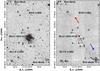 |
Fig. 1 H2 and continuum-subtracted H2 images (left and right panels) of the IRAS 13481-6124 jet. This jet is one of the few examples of jets with small precession angles and it has asymmetric lobes. Source and knots positions are indicated in the figures. Blue and red lobes are also reported according to Kraus et al. (2010). |
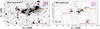 |
Fig. 2 Same as in Fig. 1 but for the IRAS 14212-6131 flow. This object represents a good example of precessing flow with only one detected lobe. The thin dashed lines show the measured precession angle. The positions of sources, knots, masers, EGOs, and H ii regions are indicated in the figures. |
As an example of the complex and different flow morphologies observed in our sample, Figs. 1–3 present three different examples: a) the IRAS 13484-6124 flow with small precession angle (8°) and asymmetric lobes (Fig. 1); b) the IRAS 14212-6131 flow with large precession angle (32°) and single lobe (Fig. 2); c) the G 35.2N flows, one of the best examples of binary precessing jets in the sample (Fig. 3).
Left and right panels in the figures show the H2 and continuum-subtracted H2 images of the targets, respectively. The positions of the sources, detected knots, known masers, EGOs as well as H ii (HC-, UC- or H ii) regions reported by SIMBAD are also labelled in the figures. The images of the remaining jets and a detailed description of the morphology of each object, including the aforementioned targets, are given in Sects. B.1–B.14 in the Appendix.
Because we do not have any kinematic information on the observed knots, our criterion to associate the H2 emission with a particular source relies entirely on the observed morphology. More precisely, our main criteria are: a) the presence of bow shocks indicating the position of the driving source; b) the collimation of jets and knots along the flow with respect to the position of the driving source; c) the measured precession angle not exceeding values of 90°.
In this paper, we define the current jet position angle (or jet position angle) as the angular offset between the knot closest to the source and the driving source itself (counterclockwise, north to east). In principle, these knots represent the most recent ejecta, therefore they provide the current PA of the jet. It is also worth noting that throughout the paper the term precession angle refers to the overall opening angle of the flow, estimated by considering the position of the driving source and the peak positions of the two most external knots at each side of the jet axis (see dashed lines in Fig. 2, right panel). Strictly speaking, the definition of precession angle should only be applied to wiggling jets, but in some cases we observe jet bending and precession (see e.g. Fig. B.11), jet bending alone (see e.g. Fig. B.9) or even more complex morphologies. Indeed, in a few objects, the apparent precession might be just a visual effect due to multiple flows.
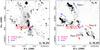 |
Fig. 3 Same as in Figs. 1 and 2 but for the G 35.2N flows. This is one of the best examples of binary jets detected in our sample. |
Often two or more flows are recognised in the observed area, and, in four out of fourteen sources (IRAS 12405-6219, IRAS 15394-5358, IRAS 16122-5047 and G 35.2N; Appendices B.2, B.8, B.10, and B.14), two jets driven by the same source are detected. Although the sources are not spatially resolved, the detection of two jets indicates the presence of a binary or multiple system, as often observed in massive star forming regions (see e.g. Kumar et al. 2002; Zinnecker & Yorke 2007; Varricatt et al. 2010). Therefore, the total number of analysed flows in this paper is eighteen.
The H2 flows recognised in our sample typically display large precession angles, up to ~60° (see e.g. Figs. 2 and B.11), much larger than those observed in low-mass jets, which are usually well collimated or with small precession angles <10° (see e.g. Caratti o Garatti et al. 2006; Arce et al. 2007). In our sample only four out of eighteen flows have precession angles smaller than 10° (see Col. 2 of Table 3; see e.g. Figs. 1 and B.4). On the other hand, the jet projected lengths on the sky (Col. 3 of Table 3) range from one tenth up to seven parsecs, which are values typically observed also in low-mass flows (e.g. in HH 34 or HH 111; see e.g. Bally & Devine 1997, and references therein). H2 bipolar flows are detected in eleven out of the eighteen analysed jets (the number of lobes detected are given in brackets in Col. 3 of Table 3). Seven flows show emission (above a 3σ threshold) only from one lobe, as also observed in other surveys of jets from intermediate- and high-mass YSOs (see Kumar et al. 2002; Varricatt et al. 2010). This is probably due to the high extinction towards the sources. Therefore the undetected lobes are more likely the red-shifted ones, where a higher AV value is expected. In two out of seven of these targets (i.e. IRAS 14212-6131 and GLIMPSE G035.0393-00.4735) there is a marginal detection (below 3σ) of the second lobe (see also Figs. 2 and B.14, and discussion in Appendices B.5 and B.13).
It is worth noting that the majority of the jets is not easily detectable without subtracting the continuum emission from the narrow band images. Firstly, the extended and bright scattered emission originating from nearby sources or by the driving source itself may conceal the emission from the jets. Secondly, the observed YSOs are located at low galactic latitudes (i.e. in highly crowded fields), and at large distances (i.e. the angular extent of the observed H2 knots is often comparable with the measured seeing in our images, ~1″). Moreover, the morphology of these flows is generally more complex than that of low-mass counterparts, because of their large precession angles, and, in some cases, the asymmetric geometry of the two lobes, or the non-detection of one of the lobes.
The jet driven by IRAS 13484-6124 (Fig. 1, see also Appendix B.3) is a clear example of a highly collimated bipolar jet in our sample (precession angle ~8°). Despite its collimation, the jet is asymmetric, namely the red-lobe is about 1.3 times more extended than the blue lobe. A possible explanation might be that the density of the interstellar medium in the blue lobe (SW of the source) is higher than in the red lobe. As a consequence, blue-shifted knots would have a lower velocity than the red-shifted ones (see also discussion in Sect. 5.2).
Figure 2 provides an example of a highly precessing flow with a single lobe. Bright continuum emission (see left panel), depicting the outflow cavity, is detected close to the driving source (G313.7654-00.8620; see also Appendix B.5), along with a more extended continuum, produced by a bright young star (2MASS J 14245631-6144472), at about 39″ WNW from the source position. After subtracting the continuum (Fig. 2, right), one of the two precessing lobes (Knots 1–4, likely the blue-shifted lobe, precession angle ~32°) of G313.7654-00.8620 is detected westwards of the source position. The second lobe is not clearly detected, likely because of the high extinction towards the target. More H2 emission, namely Knot 5, is detected towards WSW, likely driven by another YSO (i.e. 2MASS J14245547-6145227; see details in Appendix B.5) marked in Fig. 2.
As illustrated in Fig. 3, the presence of multiple jets in the same region may also confuse the morphology of the flows. The observed H2 emission was originally recognised as an hourglass shape with a large opening angle of ~40° (Lee et al. 2012), interpreted as the outflow cavities of G 35.2N. On the basis of our H2 imaging and NIR spectroscopic analysis as well as additional data from the literature, we conclude that this emission belongs to two distinct precessing jets (see Appendix B.14), likely driven by two different HMYSOs, as also suggested by ALMA interferometric observations (see Sánchez-Monge et al. 2013).
4.2. SEDs of the driving sources
From the literature we retrieved estimated distances, SEDs and bolometric luminosities for the majority of the driving sources in our sample (see Table 1). In five cases, namely G316.762-00.012, Caswell OH 322.158+00.636, IRAS 16122-5047, BGPS G014.849-00.992 and GLIMPSE G035.0393-00.4735, we construct the SEDs from the collected photometry to estimate the bolometric luminosity of each source, under the assumption that a single object dominates the luminosity of each region. The tables listing the available photometry are presented in the Appendix (see Sect. B). In each table, we report wavelengths, fluxes and uncertainties as retrieved from the catalogues. No colour correction has been applied to the data. For each object, we assume the distance reported in Table 1 and then derive its bolometric luminosity by fitting the observed SED with the radiative transfer model developed by Robitaille et al. (2007) (see e.g. Fig. 4). The model assumes a YSO with a circumstellar disc, embedded in an infalling flattened envelope with outflow cavities. The on-line tool gives the best fit from a large collection of pre-computed model SEDs. The fit provides robust estimates of the SED integrated quantities, such as the bolometric luminosity. Along with the photometric dataset, the employment of this tool requires a range of values for the distance and the foreground extinction. For the distance, we adopted the values given in Table 1. For the foreground extinction, we assumed the range of AV values measured along each flow (Table 3).
An example of our SED analysis is presented in Fig. 4. The solid black line in Fig. 4 indicates the best-fitting model for Caswell OH 322.158+00.636. Our analysis provides us with an Lbol value of ~1.3 × 10⁵ L⊙, roughly corresponding to an O7 ZAMS star of ~30 M⊙. This is the most luminous and massive object in our sample; a detailed description of this source is given in Appendix B.7. The results of the SED analysis and the figures of the four remaining SEDs are given in Appendix B.
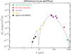 |
Fig. 4 Spectral energy distribution of Caswell OH 322.158+00.636 constructed with all photometric data available from the literature, namely from 3.6 μm to 870 μm, and by assuming a distance of 4.2 kpc to the source (Urquhart et al. 2013). The SED was fitted with the radiative transfer model developed by Robitaille et al. (2007). The fitting tool is available at http://caravan.astro.wisc.edu/protostars/. The solid black line indicates the best-fitting model. |
4.3. Spectroscopy
In Tables B.1–B.19 (see Appendix, Sect. B), we report, for each target, the fluxes (uncorrected for the extinction) of the identified lines together with their vacuum wavelengths. The line fluxes were obtained by fitting the profile with one, or two Gaussians in case of blending. The associated errors are derived from the RMS of the local baseline multiplied by the line-widths. These are typically unresolved and therefore comparable with the instrumental profile width. Lines showing fluxes with a signal-to-noise ratio (S/N) between 2 and 3, as well as those blended, have been labelled. Additional uncertainties in the fluxes are derived from the absolute calibration (≈10%).
The spectra of the jets are characterised by emission lines from molecular, i.e. H2, and atomic species, mostly [Fe ii]. These NIR lines have usually a shock origin and are always observed in protostellar jets (from both low- and high-mass YSOs; Caratti o Garatti et al. 2006, 2008), tracing the jet axis. Usually H2 or [Fe ii] lines trace different shock conditions, namely non-dissociative or dissociative shocks. The H2 lines are detected in all the observed knots, and they originate from different upper vibrational levels, namely from v = 1 to v = 3. As expected, the most prominent features are the 1–0 S(1) at 2.12 μm and the 1–0 Q line series between 2.4 and 2.5 μm. No H2 line has been detected in the blue part of the spectra (0.95−1.65 μm), except in Knots 4−5 in G 35.2N, where the 2–0 S(5) transition at 1.08 μm is marginally detected (2 <S/N< 3). This suggests that the flows are highly reddened.
[Fe ii] features are detected in 50% of the flows and in about 30% of the observed knots (20 out of 65), all showing the bright transition at 1.644 μm. In some cases (7 out of 20 knots), other fainter lines in the H band, such as the 1.534, 1.600, 1.664, 1.677 μm lines, are observed. The 1.257 μm [Fe ii] line is detected along the blue-shifted lobe of flow I in G 35.2N (see Fig. 3), where also the [C i] doublet at ~0.98 μm is observed (Knots 4 and 5). This line typically traces the neutral gas beyond the ionisation front (Hollenbach & McKee 1989), and it has often been detected in shocks in association with [Fe ii] emission (Nisini et al. 2002). Notably, we additionally detect two 2P→4P [Fe ii] lines in the K band spectral segment of the IRAS 14212-6131 source. These lines have seldom been observed close to the jet driving sources in the case of low-mass YSOs (Takami et al. 2006; Garcia Lopez et al. 2008). They have excitation energies higher than for those in the H band (26 000 vs. 11 000 K), and they are produced in highly dense and excited shocked regions, therefore they can be used to investigate the jet/wind-launching regions.
The detection of Brγ emission in a few knots (namely Knot 4 in IRAS 14212-6131, Knots 4 and 5 in G 35.2N, and Knot 1 in IRAS 13484-6100; Appendices B.5, B.14, and B.4, respectively) is also noteworthy. The location of these knots is not associated with the position of any HMYSO. In addition, these features are not spatially extended, therefore they are likely produced by shocks rather than emitted by H ii regions (e.g. Garcia Lopez et al. 2008, see also discussion in Sect. 5.1).
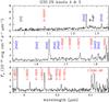 |
Fig. 5 0.95–2.5 μm SofI spectrum of Knots 4 and 5 in the G35.2N outflows. An asterisk near the line identification marks the detections between 2 and 3 sigma. Telluric lines are indicated by the symbol “⊕”. |
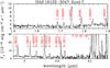 |
Fig. 6 1.5–2.5 μm SofI spectrum of Knot C in the IRAS 16122-5047 flow. Labels are as in Fig. 5. |
Our slits also encompass the positions of thirteen out of fourteen driving sources (all targets but Caswell OH 322.158+00.636). In most of the cases, the faint NIR continuum from the source comes from emission reflected by the outflow cavities or by the circumstellar material. In twelve out of thirteen targets (all but IRAS 16547-4247, whose continuum is not detected in our spectra), the spectra show steeply rising continua, indicative of highly reddened sources. In most of the cases (10 out of 13) the YSOs have also emission lines. In just one case, i.e. IRAS 15394-5358, we detect H i photospheric lines in absorption. The absence of photospheric lines in the other objects is due to the strong veiling. The most prominent emission lines come from shocks along the jet, i.e. H2 (detected in 10 targets) and [Fe ii] (6 out of 10 targets) (see e.g. Nisini et al. 2002; Caratti o Garatti et al. 2006), YSO accretion or inner winds, i.e. H i (6 out of 10 targets) (see e.g. Muzerolle et al. 1998; Natta et al. 2004; Caratti o Garatti et al. 2012), or inner disc region, namely Na i and CO (detected in 2 targets) (see e.g. Ilee et al. 2013). These lines are typically observed in HMYSOs (see e.g. Cooper et al. 2013). Notably, the only fluorescent line, the Fe ii feature at 1.688 μm, pumped by the Ly α line (Lumsden et al. 2012; Caratti o Garatti et al. 2013) and frequently detected in the NIR spectra of HMYSOs (26% of detection rate in Cooper et al. 2013), is observed only in IRAS 13481-6124 (see Table B.3), clearly one of the least reddened and most evolved HMYSO in our sample. This evidence, along with the high detection rate of jet line tracers on source, may indicate that, on average, our targets are less evolved than those presented by Cooper et al. (2013).
For the sake of simplicity, we gathered the observed spectra in three groups: 1) spectra of knots with both ionic and H2 emission; 2) spectra of knots with only H2 emission; 3) YSO spectra. These groups are summarised in Figs. 5–7, respectively.
Figure 5 shows the combined spectrum (0.95–2.5 μm) of Knots 4 and 5 along the flow I of G 35.2N, positioned NE with respect to the driving source (see also Fig. 3). The spectrum displays several H2 and [Fe ii] lines, labelled in red and blue, respectively, as well as faint emission from [C i] and H i, in black. Figure 6 displays the spectrum (1.5–2.5 μm) of Knot C in the IRAS 16122-5047 flow (see also Fig. B.9). The spectrum shows only H2 emission, labelled in red. Finally, Fig. 7 gives an example of our YSO spectra, namely the 1.5–2.5 μm SofI spectrum of G 35.2N, which partially includes emission from Knot 2, positioned ~1.5″ NE from the source. Indeed, in some cases, due to the seeing, it is not possible to disentangle the emission of nearby knots from the YSOs spectra. These cases are labelled “YSO + knot name” in our tables (see Appendix B).
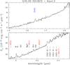 |
Fig. 7 1.5–2.5 μm SofI spectrum of G 35.2N source, which partially includes emission from Knot 2. Labels are as in Fig. 5. |
4.3.1. Jet physical parameters from the H2 analysis
The analysis of both H2 and [Fe ii] lines detected in our spectra provides quantitative information about the reddening towards the emitting regions and the excitation conditions along the jets. In particular, for each knot, we construct H2 ro-vibrational diagrams (Boltzmann plots) to derive column density, visual extinction, and temperature of the gas. To achieve it, we apply the same technique as in our previous papers on protostellar jets (see e.g. Caratti o Garatti et al. 2006, 2008).
An example of the ro-vibrational diagram for one of the observed spectra (Knot C in the IRAS 16122-5047 flow) is presented in Fig. 8 (see also the spectrum in Fig. 6). For each observed H2 transition, we plot the natural logarithm of the column density of the molecules (Nv,J) in the upper energy level (Nv,J = 4πIv,J/ (Av,Jhνv,J), where Iv,J, Av,J, and νv,J are the intensity, Einstein coefficient, and frequency of the transition, respectively) divided by its statistical weight, gv,J, against its energy level (Ev,J). To minimise the uncertainties, we only consider unblended lines with S/N ≥ 3.
If the gas is close to the local thermal equilibrium (LTE), then the H2 population follows the Boltzmann distribution i.e. Nv,J/gv,J ∝ exp( − Ej/kTex). Data points in the diagram are therefore distributed on a straight line, and an estimate of the gas excitation temperature (Tex) and the average gas column density (N(H2)) can be derived by fitting the data. This is the case observed in the majority of the ro-vibrational diagrams of our spectra, where lines with excitation energies lower than 15 000−16 000 K are detected. These are transitions originating from the vibrational levels v = 1 and v = 2, usually detected in the H and K bands. In this case a single temperature, typically between 2000 and 3000 K, can account for the observed excitation diagrams.
On the other hand, there is not much evidence of temperature stratification in our sample. Namely, only four out of 65 knots show transitions v ≥ 3, i.e. with excitation energies higher than 16 000 K. These high vibrational states are sensitive to higher temperatures, typically between ~3000 and ~4000 K (see e.g. Giannini et al. 2002, 2004). Unfortunately, many of these bright transitions are located in the J band and cannot be detected in highly reddened objects as in our sample (AV> 5–10 mag). Therefore, for these four knots, we have to rely on the faint v = 3 transitions in the K band. Here, two different temperatures are derived by fitting the v = 1, and v = 2 plus v = 3 vibrational states. Additionally, a single fit through all the lines is obtained, giving a measurement of the average temperature, which is then reported in our Tables.
An optimal value of the visual extinction (AV) can be inferred by varying the extinction values and maximizing the goodness of each fit. To deredden the observed line fluxes, we adopt the standard reddening law from Rieke & Lebofsky (1985). Because the random scatter of data points about the fit is mainly due to extinction, by varying the extinction values and maximising the goodness of each fit, an optimal AV value can be inferred. This method is typically adopted when several lines from the same vibrational level are detected, and, in general, it is more reliable than using the 1–0 S(i)/1–0 Q(i+2) ratios, because the 1–0 Q(i) transitions lie in a region of the K-band (2.4–2.6 μm) with poor atmospheric transmission (Davis et al. 2004; Giannini et al. 2004; Caratti o Garatti et al. 2006).
In Cols. 4–6 of Table 3 we report the range of average temperatures, column densities, and visual extinctions derived in each flow of the sample. The values computed for each individual knot are reported in Table A.1. Measured temperatures range from 1500 to 3300 K, with typical values around 2400–2500 K. The measured visual extinction values spread from 1 to 50 mag, with an average value around 15 mag. Column density values from this warm component range from 1017 to 1020 cm-2, with an average value of ~8 × 1018 cm-2. Notably, the values of these physical parameters are, on average, much higher than those measured in low-mass jets (see e.g. Caratti o Garatti et al. 2006).
Finally, the analysis of all the ro-vibrational diagrams suggests that the H2 emission from the observed knots is fully thermalised, i.e. it has a shock-heated origin, independently of the Lbol of the YSO. Indeed, fluorescence does not seem to be responsible for the detected emission along the flows, as suggested by the absence of high vibrational states transitions (namely, v ≥ 6) and the large values of the 1–0 S(1)/2–1 S(1) and 1–0 S(1)/3–2 S(3) dereddened ratios (≥10 and ≥100, respectively; see e.g. Takami et al. 2000; Davis et al. 2004; Caratti o Garatti et al. 2008). This result is supported by the absence of fluorescent lines observed in the HYMSOs spectra, except for IRAS 13481-6124 (see Sect. 4.3, Appendix B.3, and Table B.3). Stecklum et al. (2012) report H2 fluorescent emission in the immediate surroundings of this source (within ~5″), but beyond a few arcseconds from the source, the H2 emission along the jet is strictly thermalised, as also detected in our SofI spectra, indicating that the circumstellar material around the source screens its FUV emission. The lack of fluorescent emission along massive jets was already noted in a few previous papers, which analysed NIR spectra from individual jets (see, Davis et al. 2004; Gredel 2006; Caratti o Garatti et al. 2008). Nevertheless, this is the first time that such analysis is conducted on a large sample of intermediate- and high-mass jets.
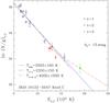 |
Fig. 8 Ro-vibratational diagram of Knot C in the IRAS 16122-5047 outflow. Different symbols indicate lines coming from different vibrational levels, as coded in the upper-right corner of the box. The three straight lines represent the best fit through the whole dataset (blue solid line), the v = 1 level (black dashed line), and v = 2,3 levels (red dashed line), respectively. The corresponding temperatures are also indicated in the lower-left corner of the box. |
Parameters of the jets of the sample derived from the H2 analysis.
4.3.2. Jet H2 luminosities and masses
Our previous analysis allows us to estimate the H2 luminosity (LH2) from the HMYSO jets. Given the large number of H2 emission lines in our NIR spectra, we expect that LH2 represents a significant fraction of the overall energy radiated away during the gas cooling in these jets. Previous studies indicate that this is the primary coolant in protostellar jets at NIR wavelengths (see also Caratti o Garatti et al. 2006, 2008).
To derive LH2, we follow the same method as in Caratti o Garatti et al. (2006). First, from our H2 images we identify and associate each knot with its driving source (see Sect. 4.1 and Sect. B). Second, the emitting area and flux of each knot are then evaluated by performing photometry on the flux calibrated continuum-subtracted H2 image. Aperture photometry is achieved with the task polyphot in IRAF, after defining each region within a 3σ contour level above the sky background. Identified knots along with their coordinates, 2.12 μm fluxes, uncertainties, and projected areas in the sky, are reported in the Appendix (Cols. 1–6 of Table A.1). Third, the AV(H2) and T(H2) values derived from our spectroscopy (Sect. 4.3.1 and Table A.1) are then used to deredden the 2.12 μm line flux and to derive the intensities of all H2 lines by applying a radiative code with gas in LTE (see details in Caratti o Garatti et al. 2006, 2008).
For those knots associated with a particular flow but not encompassed by any slit, we adopt an average value of the physical parameters derived from the flow knots. Then, for each considered knot, our LTE code provides: a) the line intensities involving levels with 0 ≤ v ≤ 14 and 0 ≤ J ≤ 29 (Ev,J ≤ 50 000 K); b) the total H2 intensity; and c) the H2 luminosity by assuming the distance to the source provided in Table 1. This process is repeated for all the knots associated with each flow, to estimate LH2 of the flow. LH2 values are reported in Col. 7 of Table 3. The inferred values range from 0.5 to 45 L⊙. This roughly reflects the large Lbol range in our sample. It is worth noting, however, that the inferred LH2 values might be lower limits of the real values, because our estimate does not take into account part of the emission from the cold H2 component, traced by the pure rotational lines in the mid-infrared (MIR) (Caratti o Garatti et al. 2008), that usually have temperatures lower and column densities higher than its NIR counterpart. Moreover, in some cases, we do not detect any emission from one lobe, likely due to the high extinction.
The final step of our H2 analysis consists in deriving a rough estimate of the mass of the H2 emitting region, by assuming Mk = 2 μmHN(H2)kAk, where μ is the average atomic weight, mH is the proton mass, N(H2)k is the H2 column density, and Ak is the area of each given knot (k). The mass of the H2 emitting regions estimated for the knots detected in our images are given in the Appendix A (Col. 10 of Table A.1), and range from 0.01 to 3.7 M⊙. As for the LH2 values, we note that these estimates are derived from the warm H2 component, which has a column density lower than the cold H2 component (Caratti o Garatti et al. 2008).
4.3.3. Jet physical parameters from the [Fe ii] analysis
For a few knots (5 out of 65), where several [Fe ii] lines (with S/N ≥ 3) have been observed, AV and the electron density (ne) can also be inferred (see e.g. Nisini et al. 2002). To estimate AV (Knots 3 and 4−5 of G 35.2N), we use the 1.257 and 1.644 μm lines, that originate from the same upper level. Their observed ratios depend only on the differential extinction. Their theoretical intensities are derived from the frequencies and Einstein coefficients of the transitions, taken from Nussbaumer & Storey (1988). As for the H2 analysis, we adopt the Rieke & Lebofsky (1985) extinction law to correct for the differential extinction and compute AV. The values derived from the [Fe ii] and H2 lines agree within the uncertainties (see Tables 4 and A.1).
To infer the electron density, we use four different line ratios from the brightest transitions in the H band, which are sensitive to density variations, namely 1.644 μm/1.533 μm, 1.644 μm/1.600 μm, 1.644 μm/1.677 μm (Nisini et al. 2002; Takami et al. 2006; Caratti o Garatti et al. 2013). For each ratio an estimate of ne is derived and a weighted mean of the various estimates is reported in Col. 3 of Table 4.
5. Discussion
First of all, it is worth noting that our sample is composed of YSOs, whose Lbol represent late B to late O ZAMS spectral types, with theoretical stellar masses (M∗) ranging from ~6 M⊙ to 25–30 M⊙. As described in Sect. 2, these targets were selected on the basis of EGO and H2 emissions, detected in previous surveys. Therefore our sample is biased towards intermediate and high-mass YSOs with bright jets and flows, and it should not be considered representative of all intermediate and high-mass YSOs.
Parameters of the jets of the sample derived from the [Fe ii] line analysis.
5.1. The shocked nature of the massive H2 jets
Our spectroscopic survey provides an answer to the important question about the nature of the H2 emission from HMYSOs. In the sample analysed, the H2 emission clearly originates from shocks at high temperatures (2500–3000 K) and with high column densities (1018−1020 cm-2), as suggested by our ro-vibrational analysis (see e.g. Fig. 8). Our spectroscopic analysis indicates that H2 is the major coolant of these flows at NIR wavelengths. Most of such emission, 70% of the analysed knots, is likely produced by non-dissociative C-type shocks, because of the high medium density and because no ionic emission is detected (Draine 1980; Giannini et al. 2004). We might speculate that in some cases the high visual extinction (AV> 25–30 mag) could prevent us from detecting the [Fe ii] emission line at 1.64 μm, which is the brightest [Fe ii] line at NIR wavelengths. Nevertheless, it is worth noting that [Fe ii] is detected in the most reddened knot of our sample (Knot 1 of Caswell OH 322.158+00.636, AV = 50 mag; see Table A.1 and B.8).
On the other hand, 30% of the knots show both atomic and molecular emissions, indicating the presence of J-type dissociative shocks (see Hollenbach & McKee 1989; Gredel 1994; Nisini et al. 2002). Remarkably, the majority of these knots originate from the most luminous (and likely most powerful) YSOs in our sample. In this case, fast shocks dissociate the molecules and destroy the grains along the flow, ionising the medium and producing the observed [Fe ii] emission. Besides, the observed H2 emission in these knots arises from oblique shocks, where the shock velocities are lower (e.g. wings of the bow-shocks, as in the red-lobe bow-shocks A and B of IRAS 13481-6124), or from reverse shocks, where the molecules are re-forming in the cooling post-shock regions behind the dissociative shocks (see e.g. Hollenbach & McKee 1989; Nisini et al. 2002; McCoey et al. 2004). Although atomic and molecular emissions are physically detached, in most of our spectral images both emitting regions are spatially coincident, because of the SofI low spatial resolution and because of the large distances involved.
Additionally, in three out of 65 knots, namely Knot 1 in IRAS 13484-6100, Knots 4+5 in G35.2N, and Knot 4 in IRAS 14212-6131 (see Table B.4, B.19, and B.5, respectively), Brγ emission is also detected. Such emission is not associated with any YSO, as in other emanations, and it is rarely detected in knots (e.g. Garcia Lopez et al. 2008). It may arise from photoionisation (Takami et al. 2000) or from the most extreme shock conditions, as in strong J-type shocks, with high shock velocities (vs ≥ 60 km s-1) and high pre-shock densities (nH ≥ 5 cm-3), which form a UV precursor that dissociate or ionise the pre-shocked gas (see e.g. Hollenbach & McKee 1989; McCoey et al. 2004). The observed emissions are compact (1–2 arcsec2), so they are more likely originating from a shock. In such a case, the expected Brγ flux can be estimated as a function of vs and nH (Burton et al. 1989; Fernandes et al. 1997):
 (1)The Brγ line fluxes from Knot 1-IRAS13484-6100 and Knots 4+5-G35.2N, and Knot 4 in IRAS 14212-6131, corrected for visual extinction (see Table A.1), are 1.8±0.5×10⁻¹⁴ (emitting area ~2 arcsec2), 5.4 ± 1.9 × 10⁻¹⁵ erg s-1 cm-2 (emitting area ~1 arcsec2), and 6.2 ± 1.2 × 10⁻¹⁵ erg s-1 cm-2 (emitting area ~1 arcsec2), respectively. Such values are compatible with J-type shocks with vs ~ 90 km s-1 (Knot 1-IRAS13484-6100), and vs ~ 60 km s-1 (Knots 4+5-G35.2N and Knot 4-IRAS 14212-6131), moving in a pre-shocked medium of nH ~ 5 cm-3.
Combining imaging and spectral analysis, we note that most of the H2 emission is detected along the flows, tracing the direction of the jet, whereas some emission, observed nearby or on source, likely traces possible outflow cavities. In conclusion, the observed shocked emissions originate from different mechanisms, namely oblique shocks from non-collimated winds (emission from the outflow cavities nearby the source) and magnetically collimated flows (along the jet). Conversely, the atomic emission is always detected along the jet axis. The observed flows move in a dense and highly inhomogeneous medium, as suggested by the range of observed column densities (1017–1020 cm-2). Our analysis indicates that, on average, both visual extinction and gas column density are highest towards the source position and decrease along the flow.
Finally, it is worth asking why no relevant fluorescent H2 emission is detected. Our previous reasoning demonstrates that the absence of strong UV radiation fields towards the observed jets is the main reason. Indeed, the HMYSOs in the sample are relatively young and they mostly lack of strong PDRs or H ii regions in the surroundings. Although some HMYSOs do possess HC- or UC-H ii regions, the high visual extinction possibly screens the UV emission from the central source. Alternatively, in some cases the absence of UV emission might be also abscribed to high accretion rates (>10-3M⊙ yr-1; see e.g. Hosokawa et al. 2010), which inflate the stellar radii up to several hundreds R⊙, producing lower effective temperatures and stellar UV luminosities.
5.2. The morphology of the massive jets
The morphology of the detected flows appear to be quite varied, ranging from a simple straight bipolar geometry to a more complex one, as monopolar, highly precessing and with patchy structures. Such a variety has been detected in many other surveys of H2 massive flows (see Kumar et al. 2002; Stecklum et al. 2009; Varricatt et al. 2010; Lee et al. 2013), as well as in many low-mass protostellar jets (see e.g. Reipurth & Bally 2001). As a matter of fact, many low-mass YSOs are not born as single, isolated stars, nor they form in a relatively still and homogeneous environment. As a consequence, straight symmetric jets from low-mass YSOs, such as HH 212 (Zinnecker et al. 1998), are not the most common. Indeed, several factors play a fundamental role in shaping the jet/flow morphology: the environment and the dynamical interactions among YSOs; the high medium density and its inhomogeneities; the large extinction values; the different evolutionary stages of the YSOs; the presence of multiple driving sources (see e.g. Eislöffel 2000; Peterson et al. 2011). These elements are largely present in high-mass star forming regions, which have extremely complex, dynamic, and inhomogeneous environments (see e.g. Zinnecker & Yorke 2007). In the following, we analyse each mechanism in the context of our observations.
-
Jet precession. HMYSOs preferentially form in clusters or small associations of YSOs. Therefore N-body interactions are likely a fundamental ingredient in the evolution of these objects as well as in shaping their flows. Changes in the flow orientation may be induced by anisotropic accretion from cores or envelopes, or by disc tilting caused by tidal interaction with close companions (Bally & Zinnecker 2005). This is the case for almost all of our jets (with the possible exception of G316.762-00.012; Appendix B.6), which show large precession angles indicating the presence of multiple systems (see e.g. Figs. 2, 3, B.1 and B.11). Notably, the large precession angles observed in our sample will likely produce poorly collimated outflows, as often observed in HMYSOs. It is worth to emphasise, however, that the mere fact of these jets having large precession, bending or showing abrupt changes in their direction does not mean that, per-se, they are not well collimated, because jets are magneto-centrifugally collimated at their base (see e.g. Pudritz et al. 2007, 2012). Jets in our sample are well collimated, even if they have large precession angles and, sometimes, a twisted geometry.
-
Jet multiplicity. In addition to jet precession, jet multiplicity also plays a role in confusing the flow morphology. In four out of fourteen sources of the sample (i.e. IRAS 12405-6219, IRAS 15394-5338, IRAS 16122-5047, and G35.2N; see Figs. B.2, B.7, B.9, and 3), or even in five if we include BGPS G014.849-00.992 whose jet multiplicity is uncertain (see Sect. B.12 and Fig. B.12), double or multiple jets have been clearly detected. Such detections allow us to infer the presence of multiple systems in spatially unresolved sources.
-
Jet asymmetry. All the observed bipolar jets display some degree of asymmetry in the two lobes, the difference in the lengths of the lobes being the most common. Pairs of ejected knots are not equally spaced from the source (see e.g. Figs. 1, 3, and B.11). It is worth noting that a highly asymmetric jet will likely produce a highly asymmetric outflow. These asymmetries are commonly observed in protostellar jets from YSOs with different masses and at different evolutionary stages (see e.g. Podio et al. 2011; Caratti o Garatti et al. 2013; Ellerbroek et al. 2014). The cause of such asymmetry is still debated, and it can be intrinsic or extrinsic to the source (see e.g. Ferreira et al. 2006; Matsakos et al. 2012). In the former case, the bipolar jet is launched at different velocities, possibly due to the asymmetric disc structure or magnetic field configuration, whereas, in the latter case, the different medium densities produce different velocities.
-
Monopolar jets/flows. H2 bipolar emission is detected above a 3σ threshold in eleven out of eighteen flows, whereas the remaining 7 flows are apparently monopolar (see Col. 3 of Table 3). However, in two out of seven cases (flows from IRAS 14212-6131 and GLIMPSE G035.0393-00.4735; see right panels of Figs. 2 and B.14) a marginal detection (between 2 and 3σ) of H2 emission from the second lobe is observed. This suggests that the higher visual extinction towards one of the lobes can hamper our observations in the NIR regime. Nevertheless, the presence of monopolar outflows from high-mass (Zapata et al. 2006; Fernández-López et al. 2013) as well as low-mass YSOs (Codella et al. 2014) has been observed in a few sources through submm outflow tracers, such as SiO and CO. The authors propose that such a monopolar geometry is due to anisotropic ambient cloud conditions or to an intrinsic asymmetry in the flow. In addition, the presence of close companion(s) might divert or even inhibit the ejection (see also Reipurth 2000; Murphy et al. 2008, and discussion therein). Unfortunately, we do not have any (sub)mm observations of theses flows to verify any of these scenarios. However, the Spitzer/GLIMPSE images show emission in excess at 4.5 μm located at the position of the undetected lobe in four out of seven flows (namely IRAS 13484-6100, IRAS 14212-6131, IRAS 15450-5431, GLIMPSE G035.0393-00.4735). Although the nature of such excess is controversial (e.g. De Buizer & Vacca 2010; Takami et al. 2012), it has been often associated with outflows (Cyganowski et al. 2008; Tappe et al. 2012).
Finally, it is worth noting that the observed flows have both extended jet emission and knotty or bow-shock structures, as those detected in low-mass jets. By assuming that these flows originate from discs and that ejection and accretion are tightly related, our observations would imply that the mass accretion rate in HMYSOs is nearly continuous with intermittent accretion outbursts, which might be identified with the observed knots and bow-shocks along the flow (see e.g. Pudritz et al. 2007). Such accretion bursts have been observed in low-mass YSOs during almost all their evolutionary stages (Caratti o Garatti et al. 2011; Audard et al. 2014), and it might be related to disc instabilities and/or dynamical interactions (see e.g. Vorobyov 2009). Furthermore, the detection of collimated jets indicates the presence of magnetic fields linked to the star/disc system, which collimates and accelerates the flows (see e.g. Pudritz et al. 2007, 2012).
5.3. H2 jets vs. sources
In this section we compare the physical properties derived from the flows with those from their driving sources. Several works discuss the interplay between the evolutionary properties of protostars and the strength of their associated outflows in both low- and high-mass YSOs (Bontemps et al. 1996; Beuther et al. 2002; Duarte-Cabral et al. 2013). In particular, Beuther et al. (2002) and Duarte-Cabral et al. (2013) derive a straightforward correlation between the momentum flux of the CO outflows (FCO) and the bolometric luminosities of HMYSOs ( ) as well as a clear relation between the envelope mass and the Lbol (
 ). If the source is accretion dominated (Lbol = Lacc + L∗ ~ Lacc) then the Lbol value is indicative of both accretion rate and mass of the source (being Lacc ~ GM∗Ṁacc/R∗). Therefore, the first relationship suggests that mass loss is mainly driven by the accretion power, which grows as the mass of the central source increases. The second correlation provides us with a relationship between the mass accretion rate and the YSO evolution. Menv is an age indicator and it is expected to decrease as the source accretes matter. By assuming that the outflow rates are somehow proportional to the accretion rates, the large FCO values found in HMYSOs indicate that their mass accretion rates must also be higher than those found in low-mass YSOs.
Additionally, Caratti o Garatti et al. (2006) evinced a tight relation between the measured molecular hydrogen flow luminosity (LH2) and the bolometric luminosities of embedded low-mass YSOs ( ), subsequently extended to a few HMYSOs (Caratti o Garatti et al. 2008). This correlation holds for very young YSOs (Class 0 and some Class I), where the bolometric luminosity is mostly coincident with the accretion luminosity of the object and implies that Ṁacc increases with the luminosity (i.e. mass) of the protostar. Observing several Class I outliers, which have less powerful H2 jets, the authors also show that the jet power decreases as low-mass YSOs evolve.
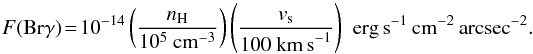
Indeed, the large H2 luminosity observed in the flows from HMYSOs suggests that high-mass protostars power the outflows at a significantly increased accretion rate, as also inferred from their higher FCO values. This trend is confirmed in our large sample. In Fig. 9 we plot the logarithmic values of flow LH2 vs. source Lbol, combining the new results of our survey (black hexagons) with those previously obtained from the HMYSO IRAS 20126+4104 (red hexagon; Caratti o Garatti et al. 2008) as well as from low-mass YSOs (red circles, blue triangles, and violet squares indicate Class 0, 0/I and I low-mass YSOs, respectively; from Caratti o Garatti et al. 2006). In the case of multiple flows from unresolved sources, we consider the total Lbol of the unresolved cores and the total LH2 from the flows. The red dashed line indicates the previous fit from Caratti o Garatti et al. (2006) with , where four low-mass outliers were excluded (see Fig. 9). The blue dashed line shows the best linear fit resulting from our HMYSO sample ( ).
).
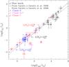 |
Fig. 9 Log(LH2) vs. Log(Lbol). Results from the current survey (black hexagons) are combined to those obtained from previous works (Caratti o Garatti et al. 2006, 2008) as labelled in the upper left corner. The red dashed line indicates the previous fit from Caratti o Garatti et al. (2006), which includes only low-mass jets and excludes the four low-mass outliers. The blue dashed line shows the best linear fit resulting from the whole sample of HMYSOs. The black dash-dotted line shows the best linear fit resulting from HMYSOs, excluding the five high-mass outliers. |
Notably the majority of the analysed HMYSOs (10 out of 15, also including IRAS 20126+4104 from Caratti o Garatti et al. 2008) agrees well with the relationship found in low-mass YSOs (red dashed line), whereas five objects are clearly positioned below. This produces a slight shift in the HMYSO fit (blue dashed line). Interestingly the five outliers (IRAS 13481-6124, IRAS 14212-6131, IRAS 15450-5431, SSTGLMC G316.7627-00.0115, and G35.2N) are among the most evolved objects in the sample, and they possess an UCH ii region. We might therefore suppose that their luminosity is no longer accretion dominated (see e.g. Smith 2014). By excluding these five outliers, we get a better agreement (black dash-dotted line) between the relationships found from low and high-mass YSOs.
Most importantly, the inferred relationship () agrees well with the correlation between the momentum flux of the CO outflows (FCO) and the bolometric luminosities of HMYSOs () from Beuther et al. (2002). This indicates that outflows from HMYSOs are momentum driven, as their low-mass counterparts (e.g. Reipurth & Bally 2001), as long as the HMYSO Lbol is accretion dominated (i.e. before or slightly after that an UCH ii region is developed).
Several observational studies of massive outflows point to an evolutionary scenario (see e.g. Beuther et al. 2002; Beuther & Shepherd 2005; Shepherd 2005), in which molecular outflows appear to loose their collimation as HMYSOs evolve from B to O spectral types. During the early B-type stage, the accreting HMYSOs drive collimated outflows, growing further in mass and luminosity, they develop UCH ii regions in the late O-type stage, and collimated jets and less collimated winds can coexist producing bipolar outflows with a lower degree of collimation. Our results show that the HMYSOs in our sample drive collimated, time-variable and highly precessing jets (e.g. Reipurth & Bally 2001). Indeed if the massive jets power their CO outflows (see also Davis et al. 2004, 2007; Arce et al. 2007; Caratti o Garatti et al. 2008), then the combined action of jet orientation variations and velocity variations may also produce poorly collimated molecular outflows.
Finally, we compare the inferred mass of the H2 jets (M(H2)) with the bolometric luminosities of their driving sources (see Fig 10; the red circles represent the five UCH ii candidates, i.e. the five HMYSO outliers of Fig. 9). In principle, M(H2) should be related to the mass of the driving source, and this can be tested through the M(H2)–Lbol relationship. Despite the large scattering, M(H2) increases with the Lbol of the source, indicating that the more massive is the source the more massive is the jet. Fig. 10 shows the best fit for the whole sample (red dashed line) and for a smaller sample, which does not include the five UCH ii candidates (blue dashed line). By excluding the five outliers, the Pearson’s coefficient increases from 0.7 to 0.9. By fitting the whole sample, we obtain the same correlation as before, namely  , whereas from the reduced sample we get
  , and the uncertainty on the exponent varies from ~40% to ~30%, respectively.
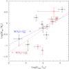 |
Fig. 10 Log(M(H2)) vs. Log (Lbol) for the sources of the current survey plus IRAS 20126+4104. The red circles are the five outliers of Fig. 9. The red dashed line represents the best linear fit to the whole sample, whereas the blue dashed line represents the best linear fit to a smaller sample, which excludes the five outliers. |
5.4. Comparing jets from low- to high-mass YSOs
Although we cannot infer the dynamical and kinematic properties of the jets, that will be analysed in a forthcoming paper, we can here provide a consistent comparison between the physical properties of jets from low-mass (Lbol ~ 0.1 L⊙) to high-mass YSOs (Lbol ~ 105 L⊙) by combining results from this and previous works (Caratti o Garatti et al. 2006, 2008).
As their low-mass counterparts, intermediate and high-mass YSOs possess collimated jets traced by line emission from shocked regions. High-mass jet tracers in the NIR are those observed in low-mass jets: H2, the major coolant, and [Fe ii]. At variance with low-mass protostellar jets, shocked Brγ emission is also detected in a few knots, indicating that here shocks can be much more powerful. In general, the physical processes, that produce such shocks, are similar, but they mostly take place in a more dense, embedded and inhomogeneous medium, therefore the environmental conditions may differ. As a result, the physical quantities derived from this study are greater than those found in low-mass objects: higher AV (10–100 mag), N(H2) (1018–1020 cm-2), TH2 (2500–3000 K), as well as larger LH2 (10–50 L⊙), and M(H2) (1–5 M⊙). These two latter quantities are strictly related to the properties of the driving source, namely higher ejection rates and more massive flows, most likely linked to the higher accretion rates of the HMYSOs. At variance with their low-mass counterparts, high-mass jets have more pronounced precession angles (up to 60°) and more confused morphologies, likely indicative of the crowded environment in which they are born. However, their outflows seem to be momentum driven as their low-mass counterparts, at least in their early evolutionary stage. Future observations at higher angular resolution and at longer wavelengths might prove the extent to which such dynamical interactions affect the jet/flow ejection.
To summarise, our analysis confirms the conclusions previously drawn from a limited sample of three jets from B-type stars (Davis et al. 2004; Gredel 2006; Caratti o Garatti et al. 2008), extending them to a larger sample with HMYSO Lbol up to ~105 L⊙: the observed high-mass protostellar jets are scaled up versions of those from low-mass protostars, albeit with some differences.
6. Conclusions
We present a NIR imaging (H2 and Ks) and low-resolution spectroscopic (0.95−2.50 μm) survey of 18 massive jets towards EGOs, observed towards the fields of 14 intermediate- and high-mass YSOs, which have Lbol between 4 × 10² and 1.3 × 10⁵ L⊙. We study the morphology of these flows, deriving their physical parameters, and we compare them with the main properties of the exciting sources, by means of literature data. The physical properties of these massive jets are also examined in comparison to their low-mass counterparts. The main results of this work are the following:
-
As in low-mass jets, H2 is the primary NIR coolant, detected in all the analysed knots. The most important ionic tracer is [Fe ii], detected in 50% of the jets and ~30% of the analysed knots. The majority of these knots originate from the most luminous YSOs, which likely drive the most powerful outflows of the sample. Brγ emission is detected in ~5% of the knots and it originates from shocks.
-
Our analysis indicates that the observed emission lines originate from shocks at high temperatures and densities. No fluorescent emission is detected along the flows, independently of the source bolometric luminosity.
-
On average, the physical parameters of these massive jets are greater than those measured in low-mass YSOs. We measure a high visual extinction towards these jets with values up to 50 mag. The excitation conditions of the jets indicate high H2 column densities up to 1020 cm-2 (1 to 4 orders of magnitude higher than the values observed in low-mass jets). On average, the temperatures traced by the rovibrational lines (v = 1 − 3) in the H and K bands are higher (~2500 K) than those typically inferred in low-mass jets (~2000 K). Inferred masses of high-mass knots are much larger than in low-mass YSOs, with values up to a few solar masses for the more massive YSOs.
-
The morphology of the detected H2 flows is heterogeneous, ranging from a simple straight bipolar geometry to a more complex one, which includes monopolar flows, highly precessing jets with patchy structures, and asymmetric lobes. Apart from the observational bias caused by the high visual extinction, such a variety depends on the complex, dynamic, and inhomogeneous environment in which these massive jets form and propagate.
-
All flows and jets of our sample are collimated, indicating a disc origin. Additionally, the presence of both knots and jets might indicate that ejection is both continuous with intermittent bursts. By assuming that accretion and ejection are tightly related, this would imply that mass accretion in intermediate- and high-mass YSOs is nearly continuous with intermittent accretion outbursts, as in low-mass YSOs.
-
We compare the measured flow H2 luminosity (the jet power) with the source bolometric luminosity (assumed representative of the accretion luminosity), confirming the tight correlation between these two quantities, already found in low-mass protostellar jets (Caratti o Garatti et al. 2006) and in the HMYSO IRAS 20126+4104 (Caratti o Garatti et al. 2008). Five sources, however, display a lower LH2/Lbol efficiency, less than one order of magnitude. We interpret this behaviour in terms of YSO evolution, i.e. their luminosity is no longer accretion dominated. Most important, the inferred relationship (
) agrees well with the correlation between the momentum flux of the CO outflows (FCO) and the bolometric luminosities of HMYSOs () from Beuther et al. (2002). This indicates that outflows from HMYSOs are momentum driven, as their low-mass counterparts. -
We also derive a less stringent correlation between the inferred mass of the H2 flows and the YSO bolometric luminosity, suggesting that the mass of the flow depends on the driving source mass. In conclusion, by comparing the physical properties of jets in the NIR, a continuity from low- to high-mass jets is identified. Massive jets appear as a scaled-up version of their low-mass counterparts in terms of their physical parameters and their origin. However, there are consistent differences, as a more variegated morphology likely due to the environment, as well as stronger shock conditions possibly due to more powerful sources.
Online material
Appendix A: Physical parameters of all observed knots
Coordinates and H2 (2.122 μm) fluxes, and physical parameters of the knots detected along the investigated flows.
Appendix B: Individual objects
Appendix B.1: [HSL2000] IRS 1
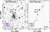 |
Fig. B.1 H2 and continuum-subtracted H2 images (left and right panels) of the [HSL2000] IRS 1 outflow. The positions of the sources, knots, masers, EGOs, and H ii regions are indicated in the figures. |
[HSL2000] IRS 1, coincident with IRAS 12091-6129, was firstly identified by Henning et al. (2000) at MIR wavelengths. The authors also detect a second source, [HSL2000] IRS 2, located ~28″ westwards. G298.2622+00.7391 is the dominant source at 8 μm. Lbol values from the literature range form 1.6 to 5.2 × 10⁴ L⊙ (Walsh et al. 1997; Henning et al. 2000; Lumsden et al. 2013), depending on the adopted distance (3.8–5.8 kpc). According to these estimates, the source spectral type ranges from B0.5 (Henning et al. 2000) to O8.5 (Walsh et al. 1997). Both CH3OH (at 6.67 GHz) and OH maser (at 1.665 GHz) emissions are detected towards the source (Walsh et al. 2001). Although reported in the SIMBAD database, it is not clear whether or not UCH ii emission is associated with this source. Walsh et al. (2001) do not detect any UCH ii region above 1 mJy at 8.64 GHz. Close to the HMYSO, Cyganowski et al. (2008) observed EGO emission (EGO G298.26+0.74), which was interpreted as scattered emission from the continuum (Takami et al. 2012). Indeed, our image (Fig. B.1) does not show any H2 emission at the EGO position. Outflow emission from CO (2–1) and CS (2–1) has been reported (Osterloh et al. 1997; Henning et al. 2000). In our image, the H2 jet is well collimated, but, possibly due to the presence of a multiple system, it shows a large precession angle (~30°). This can be easily inferred by comparing the current PA of the jet emerging from the source (PA ~ 10°) with the PA of the most distant knot (Knot 4, PA ~ − 20°). This explains why the observed CO outflow (Henning et al. 2000) has a very small collimation factor (Rc = 2.53; see Wu et al. 2004). The H2 knots are located within the CO bipolar outflow (see Fig. 1 in Henning et al. 2000), which shows spatially separated red and blue lobes, located SSE and NNW of the source. Knots 1–4 delineate the blue lobe, whereas Knots 5, and 6 are located in the red lobe (see Fig. B.1). Only H2 emission lines are detected in our spectra (Table B.1). Our slit encompasses the source position as well, where just a faint rising continuum emission is detected.
Appendix B.2: IRAS 12405-6219
Originally identified as a planetary nebula candidate from its colours (van de Steene & Pottasch 1993), it has been later recognised as an HMYSO candidate, coincident with an UCH ii region in the RMS catalogue (Lumsden et al. 2013), which reports Lbol = 3.6 × 10⁴ L⊙ at a distance of 4.4 kpc. Location of the object agrees with the position of the NIR source 2MASSJ 12433151-6236135 and that of its MIR counterpart MSX G302.0213+00.2542. NIR and MIR colours indicate that this is a young and embedded object. H2O maser emission near the source position has been reported by Suárez et al. (2009).
Our H2 image (Fig. B.2) shows the presence of several knots: Knots 1–4 are located south of the source, whereas two other knots (A and B) are aligned with the source position towards WSW. We interpret such a geometry as a combination of two distinct flows: the first flow (Knots 1–4) is precessing southwards, with a PA ranging ~170°-184°, whereas the second flow (Knots A and B) is straight with a PA of ~236°. There is no clear detection of the two opposite lobes, likely the red-shifted ones. Our spectra of Knots 1 and 2 show only H2 emission, and that on the source shows a steeply rising continuum with a bright Brγ line in emission (Table B.2).
Appendix B.3: IRAS 13481-6124
Located at a distance of 3.1 kpc (Lumsden et al. 2013), IRAS 13481-6124, spatially coincident with the NIR source 2MASS J13513785-6139075 (see also Fig. 1), was recognised as an HMYSO candidate by Chan et al. (1996), and then confirmed through the SED modelling by Grave & Kumar (2009), who obtained a stellar mass of ~20 M⊙, O9 spectral type and 6 × 10⁴ yr age. VLTI interferometric observations (Kraus et al. 2010) show the presence of a compact dusty disc with a large CO molecular outflow, driven by a parsec-scale H2 jet (Stecklum et al. 2012). Our continuum subtracted H2 image (Fig. 1) shows a precessing jet (precession angle ~8°) extending ~6.9 pc. The current PA of the jet is ~206°. The red lobe is located NE of the source and it is about 1.3 times more extended than the blue lobe. Both lobes display the same number of knots, whose distances from the source are always roughly 1.3 times larger in the red-shifted lobe of the flow, likely indicating that the red-shifted jet is moving in a less dense medium. Two large bow-shocks (A and B) are located at the apex of both lobes, whereas the remaining H2 emanations, from C to G in both lobes, have a knotty and jet-like geometry. As evinced from our analysis, visual extinction increases along the jet towards the source position, from AV = 1 to ~13 mag, whereas both T(H2) and N(H2) (i.e. temperature and column density of the shocked excited H2 gas) decrease (see Table A.1 and Sect. 4.3.1). As pointed out in Sect. 4.3.1, H2 fluorescent emission is confined within few arcseconds from the source (Stecklum et al. 2012) and the H2 emission along the jet is strictly thermalised, suggesting that the circumstellar material around the source screens its FUV emission. Our spectra indicate that H2 emission is present in all knots, whereas [Fe ii] emission is detected only in the red-shifted bow-shocks (see Table B.3).
Apart form those knots belonging to the parsec-scale collimated jet, we detect more H2 knots in our continuum-subtracted H2 image. These may belong to other flows emanating from the source position (i.e. IRAS 13481-6124 might be then a multiple system) or they might come from other YSOs. In particular, among the several H2 emanations, two knots (X and Y, see Fig. 1) are detected above a 3σ threshold and located beyond the extended nebulosity surrounding the source. Knot X, located SSE of the source, has a bow-shock shape, whose orientation might trace back to the source position. Knot Y is located NW of the source and it does not have a definite shape, therefore no definite direction is recognisable. There are no bright YSOs nearby the IRAS source, with the exception of two faint YSO candidates (about 52″ E and 55″ NW of the IRAS position), which are barely detected at 24 μm and at longer wavelengths in the Spitzer/MIPS and Herschel images. Knots X and Y might be then driven by these sources.
Our low resolution spectroscopy on the source (Fig. 1) shows many H i lines from both Paschen and Brackett series. Unfortunately, because the spectral emission in the K band is completely saturated by the source continuum, we cannot detect the Brγ emission on the source, even though it was previously detected through low-resolution spectroscopy (Beck et al. 1991), and at higher spectral and spatial resolution with SINFONI (Stecklum et al. 2012). The spectro-astrometric analysis from these data indicates that the Brγ line is spatially extended with its position angle agreeing with that of the jet. These observations as well as the detection of a collimated parsec-scale jet suggest that the source is still accreting and its disc is not just a passive disc, as proposed by Kraus et al. (2010). IRAS 13481-6124 is among the most evolved and massive objects in our sample, but possesses a powerful and collimated jet. Indeed, given the age estimate of this source (6 × 10⁴ yr; Grave & Kumar 2009), this might seem a real conundrum. In principle, the source should be evolved enough and had already developed an UCH ii region (see e.g. Zinnecker & Yorke 2007; Tan & McKee 2003). However, there are no observations of any UCH ii region around it, and ATCA observations at 3 and 6 cm do not show any radio emission down to 0.48 mJy and 1 mJy, respectively (Urquhart et al. 2007a). Moreover, by analysing the luminosity-to-mass ratio of IRAS 13481-6124 and other HMYSOs, Beltrán et al. (2006) conclude that their HMYSOs are in a pre-ultracompact H ii phase. In conclusion, IRAS 13481-6124 might not be as old as the age estimate suggests.
Observed emission lines in the [HSL2000] IRS 1 jet.
Observed emission lines in one of the two IRAS 12405-6129 jets.
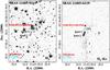 |
Fig. B.2 Same as in Fig. B.1 but for the IRAS 12405-6129 flows. |
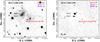 |
Fig. B.3 Same as in Fig. B.1 but for the IRAS 13484-6100 flow. |
Observed emission lines in the IRAS 13481-6124 jet.
Appendix B.4: IRAS 13484-6100
IRAS 13484-6100 is a compact GLIMPSE source (G310.1437+00.7598) with a cometary-like H ii emission, and it is located at a distance of ~5.5 kpc. CS emission (Bronfman et al. 1996), OH (Caswell 1998), CH3OH (Green et al. 2012) and H2O (Urquhart et al. 2009) masers are detected on the source and in its surroundings. Faúndez et al. (2004) detected the continuum emission from the source at 1.2 mm, and estimated Lbol = 7.1 × 10⁴ L⊙ and Mc = 1.1 × 10³M⊙ from SED analysis. On the other hand, the RMS catalogue (Lumsden et al. 2013) provides two different Lbol values of ~5 × 10³ L⊙ and 4.3 × 10⁴ L⊙ for the HMYSO and the H ii region, respectively. A bipolar EGO emission (EGO G310.15+0.76) is detected by Cyganowski et al. (2008), located ~16″ NE of the source position.
Figure B.3 shows our H2 and continuum-subtracted H2 images of IRAS 13484-6100, and Table B.4 lists the emission lines detected in the spectra. In our continuum-subtracted H2 image (Fig. B.3) the EGO emission partially overlaps with Knot 1, located at a PA of ~53° with respect to the source. A second knot (Knot 2) is observed ~4″ SW of Knot 1. From our images it is not clear whether or not these emissions belong to the same flow. Radio continuum emission at 6 cm is detected towards the Knot 1 position (Urquhart et al. 2007a). Apart from H2 emission, our spectra reveal strong [Fe ii] lines in both knots as well as towards the source position, which shows a faint raising continuum. Brγ emission from a dissociative shock (see Sect. 5.1) is also detected in Knot 1 (see Table B.4).
Observed emission lines in the IRAS 13484-6100 jet.
Appendix B.5: IRAS 14212-6131
Spitzer GLIMPSE images reveal the presence of three IR sources in this region (see Fig. 2 and discussion in Sect. 4.1). The most embedded source (G313.7654-00.8620; α(J2000) = 14:25:01.53, δ(J2000) = −61:44:57.7) is not detected in the NIR and its position agrees with that of the millimetric continuum emission observed by Faúndez et al. (2004). The IRAS position is displaced ~15″ westwards of the G313.7654-00.8620 position. The other two sources are visible at NIR wavelengths (2MASSJ 14245631-6144472 and 2MASSJ 14245547-6145227) and they are positioned ~38″ WNW and ~40″ SW of the main source, respectively. The location of the OH maser emission detected by Caswell (1998) agrees with that of G313.7654-00.8620. Assuming a distance of 4 kpc, Faúndez et al. (2004) derive a bolometric luminosity of Lbol = 1.2 × 10⁵ L⊙ and core mass (Mc) of Mc = 1.1 × 10³M⊙ from SED analysis. Lumsden et al. (2013) assume a distance of 7.8 kpc and obtain Lbol = 1.7 × 10⁴ L⊙. G313.7654-00.8620 drives the main flow of the region. CS (Bronfman et al. 1996) and CO (Urquhart et al. 2007b) emissions have been detected close to the source. H2 emission was first observed by De Buizer (2003). Four CH3OH maser spots are aligned along the flow (Walsh et al. 1997). EGO emission (EGO G313.76-0.86; Cyganowski et al. 2008) lies westwards of the source. Our continuum-subtracted H2 image (Fig. 2, right) shows four knots (1–4; suggesting an outflow with a precession angle of ~32°) driven by the central source G313.7654-00.8620. These knots are located westwards of the source, depicting the blue-shifted lobe as our ISAAC/VLT high resolution spectra indicate (Caratti o Garatti et al., in prep.). From the position of Knot 1 we infer that the current PA of the jet is ~305°. A faint H2 emission, with S/N below 3σ, appears eastwards of the source, likely depicting the red-shifted jet. As for other sources in our sample, the high visual extinction possibly prevents us from properly detecting one of the two lobes. A fifth knot (Knot 5) is detected SW from the source and it does not belong to the main flow; it is likely to be associated with a different YSO (2MASSJ14245547-6145227). The lines detected in our spectra are reported in Table B.5.
Observed emission lines in the IRAS 14212-6131 jet.
Appendix B.6: SSTGLMC G316.7627-00.0115
Positioned in the IRAS 14416-5937-B region (d = 2.8 kpc), SSTGLMC G316.7627-00.0115 was first recognised as a massive YSO candidate by Nyman et al. (2001) and Vig et al. (2007). It is located at the south-eastern end of the filamentary IRDC G316.72+0.07. This IRDC is rather pristine and just contains a few weaker MIR and FIR embedded sources (Ragan et al. 2012). The IRDC itself attains a high MIR extinction contrast (i.e. high column densities) and contains masses up to 900 M⊙ (Linz et al. 2007). SSTGLMC G316.7627-00.0115 does not seem to have a NIR counterpart, although it is quite close (~2″) to 2MASSJ 14245547-6145227, which was recognised as the NIR counterpart (Vig et al. 2007). Two OH maser emissions have been detected close to the source position (Caswell 1998). Eastwards and westwards of the source position, we detect two aligned H2 knots (1 and 2) (see Fig. B.4), whose PA is ~275 5 or ~955, depending on Knot 2 association with the blue- or red-shifted lobe, respectively. Only H2 emission lines are detected in the spectra of the two knots (see Table B.6). Our continuum-subtracted H2 image also shows the presence of a second flow ~35″ NE of the source, likely driven by a low-mass YSO. The photometric data used for our SED analysis are reported in Table B.7. Our SED analysis of SSTGLMC G316.7627-00.0115, shown in Fig. B.5, provides us with a bolometric luminosity of 5 × 10³ L⊙, at a distance of 2.8 kpc (Urquhart et al. 2013).
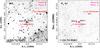 |
Fig. B.4 Same as in Fig. B.1 but for the SSTGLMC G316.7627-00.0115 flow. |
Appendix B.7: Caswell OH 322.158+00.636
The location of Caswell OH 322.158+00.636 agrees with that of the MIR source MSX G322.1587+00.6256; no NIR counterpart is detected in the 2MASS catalogue. The object is located in a very complex region, dominated at NIR wavelengths by a large nebulosity, possibly illuminated by two bright massive stars (Moisés et al. 2011). OH and CH3OH masers are detected towards the source position (Caswell 1998; Urquhart et al. 2013). In the Spitzer GLIMPSE images the source is saturated at both 24 μm and 70 μm, whereas its emission is below the linearity limit in the Herschel PACS images. A second fainter IR object, MSX5C G322.1587+00.6262, is positioned about 35″ SE of the source. In our continuum-subtracted H2 image (see Fig. B.6) we detect a bright knot (Knot 1) ~5″ SW of the source, almost coincident with a very bright EGO observed in the Spitzer/IRAC images. Our NIR spectroscopy shows both H2 and [Fe ii] emission from this knot (Table B.8). The knot position angle is ~210°. Our continuum-subtracted H2 image also shows the presence of a second bright knot, Knot 2, positioned about 68″ SE of the Knot 1. Knot 2 does not seem to emanate from MSX G322.1587+00.6256, but more likely from MSX5C G322.1587+00.6262. The retrieved photometry of MSX G322.1587+00.6256 is reported in Table B.9. By assuming a distance of 4.3 kpc (Urquhart et al. 2013), our SED analysis (see Fig. 4) provides us with an Lbol of ~1.3 × 10⁵ L⊙, roughly corresponding to an O7 ZAMS star with a mass of ~30 M⊙. Therefore this object is the most luminous and massive of our sample.
Appendix B.8: IRAS 15394-5358
IRAS 15394-5358 is part of a small cluster of YSOs, where CO (Urquhart et al. 2007b) and CS (Bronfman et al. 1996) emissions as well as CH3OH (Caswell 1998) and H2O (Scalise et al. 1989) masers are observed. Faúndez et al. (2004) detected continuum emission at 1.2 mm. By assuming a distance of 2.8 kpc, they obtained Lbol = 1.5 × 10⁴ L⊙ and Mc = 8 × 10³M⊙ from the SED analysis. On the other hand, Lumsden et al. (2013) reported a distance of 1.8 kpc and derived Lbol = 4 × 10³ L⊙.
Observed emission lines in the SSTGLMC G316.7627-00.0115 jet.
SSTGLMC G316.7627-00.0115 available photometry.
Our continuum-subtracted H2 image (Fig. B.7) shows two bright jets emanating from IRAS 15394-5358, that is surrounded by an extended nebulosity. There is a relatively bright NIR source at the centre of the nebula (2MASSJ 15431897-5407356), and an H ii region is located 15″ eastwards (Bronfman et al. 1996). In the K band image, we detect a very faint source (α = 15:43:18.945, δ = −54:07:37.84, J2000, not detected in 2MASS) ~2″ southwards of 2MASSJ 15431897-5407356. This might be the second component of the binary system that drives the two flows. The system is not resolved in the Spitzer GLIMPSE images, and we do not have any other photometric or colour information to prove the nature of this source. The first precessing jet (precession angle ~42°) is composed of Knots 2, 3, 6, 7, 8, 9 (the blue-shifted lobe; Caratti o Garatti et al. in prep.) and Knots 1 and, possibly, 10 and 11 (likely to be the red-shifted lobe). It has a C shape and it is likely driven by the brightest NIR source (2MASSJ 15431897-5407356). The PA of the jet is ~207°. The second flow is likely driven by the faintest NIR companion and shows two knots (4 and 5), roughly aligned with the faint NIR source. Its PA is ~300°, if Knot 4 is part of the blue-shifted lobe (because of its lowest visual extinction), or it is ~120°, if Knot 4 belongs to the red-shifted lobe. Our spectral analysis indicates the presence of both H2 and [Fe ii] emission along the first flow, whereas only H2 emission is detected along the second flow (see Table B.10). Finally, in our continuum-subtracted H2 image (Fig. B.7), a third H2 flow is detected. This flow is likely driven by another HMYSO, namely G326.474+0.697 (Garay et al. 2007b), which is detected at FIR wavelengths in both Spitzer and Herschel images. The flow displays several knots extending NE-SW of the source position. EGO G326.48+0.70 (Cyganowski et al. 2008) is associated with this third outflow. The flow was not encompassed by our slits and it is not discussed further in this paper.
Observed emission lines in the Caswell OH 322.158+00.636 jet.
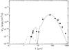 |
Fig. B.5 Spectral energy distribution (SED) of SSTGLMC G316.7627-00.0115 constructed with all photometric data available from the literature, namely from 3.6 μm to 870 μm, and assuming a distance of 2.8 kpc to the source (Ragan et al. 2012). |
Appendix B.9: IRAS 15450-5431
The location of IRAS 15450-5431 agrees with that of a bright GLIMPSE source (G326.7807-00.2409) in the MIR and with that of 2MASSJ 15485523-5440375 in the NIR. CS (Bronfman et al. 1996) and H2O maser emission (Urquhart et al. 2009) are reported close to the source location. The RMS catalogue provides a distance of 3.9 kpc and a bolometric luminosity of 9 × 10³ L⊙. EGO G326.78-0.24 (Cyganowski et al. 2008) is located close to the IR source. Our K band and H2 images (see the H2 image in Fig. B.8, left) show a cone-like nebulosity NE of the NIR source, likely depicting an outflow cavity. A precessing jet (precession angle ~33°) emerging from this outflow cavity is detected in the continuum-subtracted H2 image (Fig. B.8, right). From the position of Knot 4 we derive a jet PA of ~31°, and only one lobe, likely the blue-shifted one, is detected. Only H2 emission lines are detected along the flow in our spectra (see Table B.11). The on-source spectrum shows a bright rising continuum with puzzling H i lines from the Brackett series in absorption. Indeed there are examples in the literature where photospheric lines could be detected from the scattered light (e.g. Cohen et al. 1986; Neckel & Staude 1995).
Caswell OH 322.158+00.636 available photometry.
Appendix B.10: IRAS 16122-5047
IRAS 16122-5047 is not well studied. According to the Spitzer GLIMPSE images, IRAS 16122-5047 seems to be part of a small cluster, composed of two sources, well detected at 24 μm, and a few more fainter objects. The location of the brightest IR source in our field (GLIMPSE G332.3526-00.1154), the only one detected at 70 μm with MIPS, agrees with that of 2MASSJ 16160689-5054274. OH maser emission is detected on source (Caswell 1998) and CH3OH maser emission is detected towards EGO G332.35-0.12 (Chen et al. 2011). Two EGOs are reported by Cyganowski et al. (2008), namely EGO G332.35-0.12 close to the NIR source, and EGO G332.33-0.12, about 74″ SW of the 2MASS source. Both K band and H2 images (see H2 image in Fig. B.9, left) show some nebulosity around the 2MASS source, that might delineate an outflow cavity (towards NNE), although the geometry does not appear so clear in our images. The continuum-subtracted H2 image shows two different flows, which appear to emanate from the 2MASSJ 16160689-5054274 position. The first flow, which includes Knots A, B, C, and D, has a curved shape. Its PA, measured from Knot A position, is ~15°. The second flow includes Knots 1, 2, 3, and it has a straight geometry with a PA of ~14°. There is an additional knot (R1), which is located in the opposite direction of both flows. Therefore it is not clear as to which flow it belongs. It is likely to be part of the red-shifted lobe of one of the two flows. Only H2 lines are detected in the spectra of the knots (see Table B.12). Collected photometry is reported in Table B.13. Assuming a distance of 3.1 kpc (Urquhart et al. 2013), our SED analysis provides a bolometric luminosity of ~5 × 10³ L⊙ (see Fig. B.10).
Observed emission lines in the IRAS 15394-5358 jets.
Observed emission lines in the IRAS 15450-5431 jet.
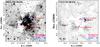 |
Fig. B.6 Same as in Fig. B.1 but for the Caswell OH 322.158+00.636 flow. |
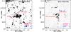 |
Fig. B.7 Same as in Fig. B.1 but for the IRAS15394-5358 flows. |
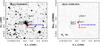 |
Fig. B.8 Same as in Fig. B.1 but for the IRAS 15450-5431 flow. |
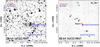 |
Fig. B.9 Same as in Fig. B.1 but for the IRAS 16122-5047 flows. |
Observed emission lines in the IRAS 16122-5047 jets.
Appendix B.11: IRAS 16547-4247
IRAS 16547-4247 or G343.126-0.062 is an isolated massive and dense core located at a distance of 2.9 kpc (Garay et al. 2003; Rodríguez et al. 2008). Its bolometric luminosity estimates range from 6.2 × 10⁴ L⊙ (Garay et al. 2003; Faúndez et al. 2004) to 6.6 × 10⁴ L⊙ (Lumsden et al. 2013, who assume a distance of 2.8 kpc to the source). These values are consistent with an O9 spectral type for a single ZAMS star. The core mass derived from the dust emission at 1.2 mm is 1.4 × 10³M⊙ (Faúndez et al. 2004). The source is not detected in our NIR images or in the Spitzer/IRAC images, although it is visible as a single object in the Spitzer/MIPS images at 24 μm. At high spatial resolution, Submillimeter Array (SMA) observations of the dust continuum at 1.3 mm (Franco-Hernández et al. 2009) trace a more complex structure, indicating that there might be at least two objects. H2O masers were detected towards the source position (Batchelor et al. 1980). SMA observations at a higher spatial resolution show that water maser emission is present in several distinct parts of the region (Franco-Hernández et al. 2009). In particular, a compact structure located at the disc position and perpendicular to the radio jet shows a velocity gradient possibly arising from Keplerian motion, which would imply a mass of ~30 M⊙ for the central star(s). The source drives a thermal radio jet, extending 0.14 pc with a PA of ~163° (Garay et al. 2003; Rodríguez et al. 2005). A parsec-scale H2 flow (MHO 1900–1902) well aligned with the radio jet was observed by Brooks et al. (2003). More recently, Garay et al. (2007b) observed a well collimated CO bipolar outflow roughly oriented in the north-south direction (the blue-shifted lobe lies southwards; see e.g. Garay et al. 2007a), close to the plane of the sky (i = 84°±2°). EGO emission (EGO G343.12-0.06) has been also detected close to the source (Cyganowski et al. 2008). As for the majority of the EGOs, such emission can be due to scattered continuum in the HMYSO outflow cavities (Takami et al. 2012).
Figure B.11 shows the H2 and continuum-subtracted H2 images from ISAAC. These data were originally presented by Brooks et al. (2003). We reduced and analysed the data again, finding similar results (e.g. calibrated fluxes are identical, within the errors). We also keep the knot nomenclature same as in Brooks et al. (2003). In addition, we detect another knot (named A6), which is also visible in their Fig. 1. This is likely the terminal bow-shock of the red-shifted lobe. Because of to the high visual extinction, no H2 emission is detected near the source position, therefore the current jet PA is not measurable. We assume a PA of 177° pm 4°, according to the observed radio jet emission (Franco-Hernández et al. 2009). The extension of the whole jet, including both lobes, is about 3.4 pc at a distance of 2.9 kpc. The jet shows one of the largest precession angle in our sample, i.e. 57° (computed from Knots B1 and B2), and the jet axis PA drifts from ~161° to 218°. Our sepectroscopic analysis reveals both H2 and [Fe ii] emission lines in the analysed knots (see Table B.14).
IRAS 16122-5047 available photometry.
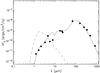 |
Fig. B.10 Spectral energy distribution (SED) of IRAS 16122-5047 constructed with all photometric data available from the literature, namely from 3.6 μm to 870 μm, and assuming a distance of 3.1 kpc (Urquhart et al. 2013). |
Observed emission lines in the IRAS 16547-4247 jet.
Observed emission lines in the BGPS G014.849-00.992 jet.
Appendix B.12: BGPS G014.849-00.992
BGPS G014.849-00.992 (α = 18:21:12.922, δ = −16:30:10.2, J2000) was first reported in the Bolocam Galactic Plane Survey (BGPS) catalogue (Rosolowsky et al. 2010). A second source (G014.8516-00.9890), located ~12″ NW of BGPS G014.849-00.992, is also detected in the Spitzer GLIMPSE images at 24 μm (see Fig B.12). This source is not spatially resolved in the Spitzer/MIPS images at 70 μm. In Herschel PACS images at 70 μm, the two sources are partially resolved, and BGPS G014.849-00.992 is the brightest source at 70 μm whereas the second source is barely detected, indicating that BGPS G014.849-00.992 is the dominant source at FIR wavelengths. Lim et al. (2012) report the detection of strong multiple H2O maser emissions along the flow as well as CH3OH maser emission close to the location of the BGPS source (~10″). None of the sources is detected in our NIR images. Two flows are likely detected in our continuum-subtracted H2 image (Fig. B.12, right). The first flow is driven by BGPS G014.849-00.992, located close to Knot 1, and it is composed of Knots 1, 2 and, possibly, 7. Its PA is ~324° or ~144°, depending on whether or not Knot 2 belongs to the blue-shifted lobe. There is a second curved flow, composed of Knots 4, 5, 6, and, possibly, 7. It is slightly misaligned with respect to the second IR source, therefore the latter might not be the driving source. It is worth noting, however, that no additional IR sources are detected in the FoV. Our NIR spectra show only H2 emission along the flows (see Table B.15). Collected photometry is reported in Table B.16. Figure B.13 shows the SED analysis of BGPS G014.849-00.992. By assuming a distance of 2.5 kpc (Csengeri et al. in prep.), best fitting model indicates an Lbol value of 1.3 × 10³ L⊙ and a central mass of ~8 M⊙, namely at the edge of the HMYSO regime.
Appendix B.13: GLIMPSE G035.0393-00.4735
GLIMPSE G035.0393-00.4735 is an IR source, observed from MIR wavelengths longward. It belongs to the IR dark cloud SDC G35.041-0.471 (Peretto & Fuller 2009). EGO emission (EGO G035.04-0.47) was detected close to the source position (Cyganowski et al. 2008). Lee et al. (2012) detect H2 emission associated with the IR source, named MHO 2429. The H2 emission is precessing and shows two lobes (see their Fig. 14), a bright one (MHO 2429 A), possibly the blue-shifted one, and a faint one (MHO 2429 B), possibly the red-shifted one. In our continuum-subtracted H2 image (Fig. B.14, right), we detect two bright Knots (1 and 2) in the lobe coincident with MHO 2429 A, and a third knot, with S/N< 3, at the location of MHO 2429 B. As for other sources in our sample, the jet emission from one of the two flow lobes is likely hampered by the high visual extinction. The jet PA is ~205° or ~25°, depending on whether or not Knot 2 belongs to the blue- or red-shifted lobe, and it has a precession angle of 22°. The spectra of the observed knots show only H2 emission (see Table B.17). Collected photometry is reported in Table B.18. By assuming a distance of 3.4 kpc, our SED analysis in Fig. B.15 provides us with an Lbol value of 2–4 × 10² L⊙ and a central mass of ~5 M⊙, suggesting that GLIMPSE G035.0393-00.4735 is an intermediate-mass YSO and not an HMYSO.
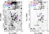 |
Fig. B.11 Same as in Fig. B.1 but for the IRAS 16547-4247 flow. |
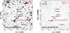 |
Fig. B.12 Same as in Fig. B.1 but for the BGPS G014.849-00.992 flow. |
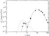 |
Fig. B.13 Spectral energy distribution (SED) of BGPS G014.849-00.992 constructed with all photometric data available from the literature, namely from 3.6 μm to 1.1 mm, and assuming a distance of 2.5 kpc to the source (Lim et al. 2012). |
BGPS G014.849-00.992 available photometry.
Appendix B.14: G35.2N
G35.20-0.74 N (G35.2N), also known as IRAS 18556+0136, is a massive star forming region at a distance of 2.2 kpc (Zhang et al. 2009). Radio continuum emission shows a collimated jet directed northwards (Heaton & Little 1988; Gibb et al. 2003). Coincident with the radio jet emission a collimated jet has been detected at NIR and MIR wavelengths (Fuller et al. 2001; De Buizer 2006; Zhang et al. 2013). An SW-NE poorly collimated CO outflow (collimation factor of 2.4–2.6, see Beuther et al. 2002; Wu et al. 2004) was first detected by Dent et al. (1985), with the blue-shifted lobe located NE of the IRAS position. Additional CO and SiO observations at higher angular resolution (Gibb et al. 2003; Birks et al. 2006) suggested the presence of multiple precessing outflows. Both papers consider this interpretation more plausible than the jet precession to explain the different jet/outflow orientations. On the other hand, Lee et al. (2012) detect an hourglass-shape H2 emission with a large opening angle of ~40° (MHO 2431) emanating from the central region and extending ~2′ SW-NE, i.e. ~1.3 pc at a distance of 2.2 kpc. They interpret this as a single outflow with a large opening angle, rather than as two distinct jets.
Indeed, it is not clear if there is just a single massive source at the centre of the region (Zhang et al. 2013) or rather a small cluster (Sánchez-Monge et al. 2013). A 0.2 pc interstellar disc-like structure was detected in H13CO+, H13CN and millimetre continuum emission (Dent et al. 1985; Gibb et al. 2003; Sánchez-Monge et al. 2013). At least three separate cores, namely G35.2N (A and B) and [GHL2003] G35MM2 (hereafter G35MM2), are clearly detected with ALMA high angular observations (see Fig. 2 in Sánchez-Monge et al. 2013). Sánchez-Monge et al. (2013) estimate a mass of ~18 M⊙ for the A/B G35.2N clumps.
Estimates of the observed bolometric luminosity are between 3.1×10⁴ and 3.3 × 10⁴ L⊙ (Lumsden et al. 2013; Zhang et al. 2013). However, Zhang et al. (2013) provide a more complex SED modelling, which takes into account both the foreground extinction and the so called flash-light effect, i.e. the loss of photons through the outflow cavities. Their Lbol estimate ranges between 7 × 10⁴ and 2.2 × 10⁵ L⊙, consistent with a single star of 20–30 M⊙. Such values, however, are in contrast with the momentum flux measured from the CO outflow, that is more than one order of magnitude smaller than expected from such a luminous object (Zhang et al. 2013). Sánchez-Monge et al. (2013) argue that a binary system with a total mass of 18 M⊙ would better fit the measured bolometric luminosities and outflow momentum flux, as well as it would better explain the jet/outflow axes displacement.
Our images indicate the presence of two main precessing jets (see Fig. 3). The first precessing jet (Knots 1–5) is launched by G35.2N, most likely from the position of clump B. Our NIR continuum images show a conical emission (PA~9°, opening angle of ~45°), which is most likely the CO outflow cavity of the blue-shifted lobe of flow I (Gibb et al. 2003; Birks et al. 2006, see also Fig. 3 and discussion in Sect. 4.1), excavated by the jet. The current jet position angle (close to the source position, YSO emission + Knot 2) is ~− 1°, i.e. coincident with the MIR and radio jet emission. The jet is then bending and precessing towards NE (Knots 3–5) with a precession angle of ~28°, in agreement with the opening of the outflow cavity. Knot 1 and the emission towards SSW seem to depict the red-shifted lobe of the jet. According to our spectroscopic analysis, the H2 knots are clearly tracing the jet axis, and not oblique shocks from an expanding shell/outflow as suggested by Lee et al. (2012), because of their excitation conditions. Most important, [Fe ii] emission is clearly detected along the whole blue-shifted part of this flow, namely in the jet inside the outflow cavity and in Knots 2–5. Such emission is produced by strong dissociative shocks and it always traces the axis of the jets (Nisini et al. 2002; Pyo et al. 2006; Shang et al. 2006; Caratti o Garatti et al. 2009), therefore it cannot be associated with any outflow cavity or expanding flow (see Table B.19). As in other flows, this jet is highly asymmetric, namely one lobe is more extended than the other (in this case the blue-shifted lobe is ~2.5 times more extended than the red one).
The second flow is composed of Knots 6 and 7, in the red-shifted lobe, and Knots 8–10, in the blue-shifted lobe. This flow has a precession angle of 26°, and, if we consider the two terminal shocks of the flow (Knot 6 and 10), the flow position angle is ~45°. We do not detect emission from any outflow cavity in our images, nor any source emission in the Spitzer GLIMPSE images, indicating that the driving source must be very embedded and young. G35.2N is not a feasible candidate because the opening angle of the outflow cavity does not match with the jet position. On the other hand, G35MM2 position lies very close (~0.̋7) to the line intersecting the two terminal shocks, therefore it is the best driving source candidate. However, given the large precession angle of the jet and the lack of H2 emission close to the launching region, we cannot exclude other embedded sources as possible candidates.
Observed emission lines in the GLIMPSE G035.0393-00.4735 jet.
GLIMPSE G035.0393-00.4735 available photometry.
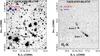 |
Fig. B.14 Same as in Fig. B.1 but for the GLIMPSE G035.0393-00.4735 flow. |
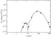 |
Fig. B.15 Spectral energy distribution (SED) of GLIMPSE G035.0393-00.4735 constructed with all photometric data available from the literature, namely from 3.6 μm to 1.1 mm, and assuming a distance of 2.5 kpc to the source (Lim et al. 2012). |
Observed emission lines in the G35.2N jets.
In this paper we favour the term high-mass young stellar object (HMYSO; e.g. Varricatt et al. 2010) instead of high-mass protostellar object (HMPO), because the former also includes young massive stars on the ZAMS.
IRAF (Image Reduction and Analysis Facility) is distributed by the National Optical Astronomy Observatories, which are operated by AURA, Inc., cooperative agreement with the National Science Foundation.
Acknowledgments
We are grateful to Dr. Timea Csengeri for providing us with ATLASGAL fluxes and for her help. We wish to thank an anonymous referee for useful insights and comments. This publication makes use of data products from: the Wide-field Infrared Survey Explorer, which is a joint project of the University of California, Los Angeles, and the Jet Propulsion Laboratory/California Institute of Technology, funded by the National Aeronautics and Space Administration; the 2MASS data, obtained as part of the Two Micron All Sky Survey, a joint project of the University of Massachusetts and the Infrared Processing and Analysis Center/California Institute of Technology. This research has also made use of NASA’s Astrophysics Data System Bibliographic Services and the SIMBAD database, operated at the CDS, Strasbourg, France.
References
- Arce, H. G., Shepherd, D., Gueth, F., et al. 2007, in Protostars and Planets V, 245 [Google Scholar]
- Audard, M., Ábrahám, P., Dunham, M. M., et al. 2014, in Protostars and Planets VI (University of Arizona Press), eds. H. Beuther et al., in press [arXiv:1401.3368] [Google Scholar]
- Bally, J. 2007, Ap&SS, 311, 15 [NASA ADS] [CrossRef] [Google Scholar]
- Bally, J., & Devine, D. 1997, in Herbig-Haro Flows and the Birth of Stars, eds. B. Reipurth, & C. Bertout, IAU Symp., 182, 29 [Google Scholar]
- Bally, J., & Zinnecker, H. 2005, AJ, 129, 2281 [NASA ADS] [CrossRef] [Google Scholar]
- Batchelor, R. A., Caswell, J. L., Haynes, R. F., et al. 1980, Aust. J. Phys., 33, 139 [NASA ADS] [CrossRef] [Google Scholar]
- Beck, S. C., Fischer, J., & Smith, H. A. 1991, ApJ, 383, 336 [NASA ADS] [CrossRef] [Google Scholar]
- Beltrán, M. T., Brand, J., Cesaroni, R., et al. 2006, A&A, 447, 221 [NASA ADS] [CrossRef] [EDP Sciences] [MathSciNet] [Google Scholar]
- Benjamin, R. A., Churchwell, E., Babler, B. L., et al. 2003, PASP, 115, 953 [NASA ADS] [CrossRef] [Google Scholar]
- Beuther, H., & Shepherd, D. 2005, in Cores to Clusters: Star Formation with Next Generation Telescopes, eds. M. S. N. Kumar, M. Tafalla, & P. Caselli, Astrophys. Space Sci. Lib. (New york: Springer), 324, 105 [Google Scholar]
- Beuther, H., Schilke, P., Sridharan, T. K., et al. 2002, A&A, 383, 892 [NASA ADS] [CrossRef] [EDP Sciences] [Google Scholar]
- Beuther, H., Schilke, P., & Gueth, F. 2004, ApJ, 608, 330 [NASA ADS] [CrossRef] [Google Scholar]
- Birks, J. R., Fuller, G. A., & Gibb, A. G. 2006, A&A, 458, 181 [NASA ADS] [CrossRef] [EDP Sciences] [Google Scholar]
- Bontemps, S., Andre, P., Terebey, S., & Cabrit, S. 1996, A&A, 311, 858 [NASA ADS] [Google Scholar]
- Bronfman, L., Nyman, L.-A., & May, J. 1996, A&AS, 115, 81 [NASA ADS] [Google Scholar]
- Brooks, K. J., Garay, G., Mardones, D., & Bronfman, L. 2003, ApJ, 594, L131 [NASA ADS] [CrossRef] [Google Scholar]
- Burton, M. G., Geballe, T. R., & Brand, P. W. J. L. 1989, MNRAS, 238, 1513 [NASA ADS] [CrossRef] [Google Scholar]
- Caratti o Garatti, A., Giannini, T., Nisini, B., & Lorenzetti, D. 2006, A&A, 449, 1077 [NASA ADS] [CrossRef] [EDP Sciences] [Google Scholar]
- Caratti o Garatti, A., Froebrich, D., Eislöffel, J., Giannini, T., & Nisini, B. 2008, A&A, 485, 137 [NASA ADS] [CrossRef] [EDP Sciences] [Google Scholar]
- Caratti o Garatti, A., Eislöffel, J., Froebrich, D., et al. 2009, A&A, 502, 579 [NASA ADS] [CrossRef] [EDP Sciences] [Google Scholar]
- Caratti o Garatti, A., Garcia Lopez, R., Scholz, A., et al. 2011, A&A, 526, L1 [NASA ADS] [CrossRef] [EDP Sciences] [Google Scholar]
- Caratti o Garatti, A., Garcia Lopez, R., Antoniucci, S., et al. 2012, A&A, 538, A64 [NASA ADS] [CrossRef] [EDP Sciences] [Google Scholar]
- Caratti o Garatti, A., Garcia Lopez, R., Weigelt, G., et al. 2013, A&A, 554, A66 [NASA ADS] [CrossRef] [EDP Sciences] [Google Scholar]
- Carey, S. J., Noriega-Crespo, A., Mizuno, D. R., et al. 2009, PASP, 121, 76 [NASA ADS] [CrossRef] [Google Scholar]
- Casali, M., Adamson, A., Alves de Oliveira, C., et al. 2007, A&A, 467, 777 [NASA ADS] [CrossRef] [EDP Sciences] [Google Scholar]
- Caswell, J. L. 1998, MNRAS, 297, 215 [NASA ADS] [CrossRef] [Google Scholar]
- Chan, S. J., Henning, T., & Schreyer, K. 1996, A&AS, 115, 285 [NASA ADS] [Google Scholar]
- Chen, X., Ellingsen, S. P., Shen, Z.-Q., Titmarsh, A., & Gan, C.-G. 2011, ApJS, 196, 9 [NASA ADS] [CrossRef] [Google Scholar]
- Chen, X., Gan, C.-G., Ellingsen, S. P., et al. 2013, ApJS, 206, 9 [NASA ADS] [CrossRef] [Google Scholar]
- Churchwell, E., Babler, B. L., Meade, M. R., et al. 2009, PASP, 121, 213 [NASA ADS] [CrossRef] [Google Scholar]
- Codella, C., Maury, A. J., Gueth, F., et al. 2014, A&A, 563, L3 [NASA ADS] [CrossRef] [EDP Sciences] [Google Scholar]
- Cohen, M., Dopita, M. A., & Schwartz, R. D. 1986, ApJ, 307, L21 [NASA ADS] [CrossRef] [Google Scholar]
- Cooper, H. D. B., Lumsden, S. L., Oudmaijer, R. D., et al. 2013, MNRAS, 430, 1125 [NASA ADS] [CrossRef] [Google Scholar]
- Csengeri, T., Urquhart, J. S., Schuller, F., et al. 2014, A&A, 565, A75 [NASA ADS] [CrossRef] [EDP Sciences] [Google Scholar]
- Cutri, R. M. E. 2012, VizieR Online Data Catalog: II/311 [Google Scholar]
- Cyganowski, C. J., Whitney, B. A., Holden, E., et al. 2008, AJ, 136, 2391 [NASA ADS] [CrossRef] [Google Scholar]
- Davis, C. J., Varricatt, W. P., Todd, S. P., & Ramsay Howat, S. K. 2004, A&A, 425, 981 [NASA ADS] [CrossRef] [EDP Sciences] [Google Scholar]
- Davis, C. J., Kumar, M. S. N., Sandell, G., et al. 2007, MNRAS, 374, 29 [NASA ADS] [CrossRef] [Google Scholar]
- Davis, C. J., Gell, R., Khanzadyan, T., Smith, M. D., & Jenness, T. 2010, A&A, 511, A24 [NASA ADS] [CrossRef] [EDP Sciences] [Google Scholar]
- De Buizer, J. M. 2003, MNRAS, 341, 277 [NASA ADS] [CrossRef] [Google Scholar]
- De Buizer, J. M. 2006, ApJ, 642, L57 [NASA ADS] [CrossRef] [Google Scholar]
- De Buizer, J. M., & Vacca, W. D. 2010, AJ, 140, 196 [NASA ADS] [CrossRef] [Google Scholar]
- Dent, W. R. F., Little, L. T., Kaifu, N., Ohishi, M., & Suzuki, S. 1985, A&A, 146, 375 [NASA ADS] [Google Scholar]
- Draine, B. T. 1980, ApJ, 241, 1021 [NASA ADS] [CrossRef] [Google Scholar]
- Duarte-Cabral, A., Bontemps, S., Motte, F., et al. 2013, A&A, 558, A125 [NASA ADS] [CrossRef] [EDP Sciences] [Google Scholar]
- Egan, M. P., Price, S. D., Kraemer, K. E., et al. 2003, VizieR Online Data Catalog: V/114 [Google Scholar]
- Eislöffel, J. 2000, A&A, 354, 236 [NASA ADS] [Google Scholar]
- Ellerbroek, L. E., Podio, L., Dougados, C., et al. 2014, A&A, 563, A87 [NASA ADS] [CrossRef] [EDP Sciences] [Google Scholar]
- Faúndez, S., Bronfman, L., Garay, G., et al. 2004, A&A, 426, 97 [NASA ADS] [CrossRef] [EDP Sciences] [Google Scholar]
- Fernandes, A. J. L., Brand, P. W. J. L., & Burton, M. G. 1997, MNRAS, 290, 216 [NASA ADS] [CrossRef] [Google Scholar]
- Fernández-López, M., Girart, J. M., Curiel, S., et al. 2013, ApJ, 778, 72 [NASA ADS] [CrossRef] [Google Scholar]
- Ferreira, J., Dougados, C., & Cabrit, S. 2006, A&A, 453, 785 [NASA ADS] [CrossRef] [EDP Sciences] [Google Scholar]
- Franco-Hernández, R., Moran, J. M., Rodríguez, L. F., & Garay, G. 2009, ApJ, 701, 974 [NASA ADS] [CrossRef] [Google Scholar]
- Frank, A., Ray, T. P., Cabrit, S., et al. 2014, in Protostars and Planets VI (University of Arizona Press), eds. H. Beuther et al., in press [arXiv:1402.3553] [Google Scholar]
- Fuller, G. A., Zijlstra, A. A., & Williams, S. J. 2001, ApJ, 555, L125 [NASA ADS] [CrossRef] [Google Scholar]
- Garay, G., Brooks, K. J., Mardones, D., & Norris, R. P. 2003, ApJ, 587, 739 [NASA ADS] [CrossRef] [Google Scholar]
- Garay, G., Mardones, D., Bronfman, L., et al. 2007a, A&A, 463, 217 [NASA ADS] [CrossRef] [EDP Sciences] [Google Scholar]
- Garay, G., Mardones, D., Brooks, K. J., Videla, L., & Contreras, Y. 2007b, ApJ, 666, 309 [NASA ADS] [CrossRef] [Google Scholar]
- Garcia Lopez, R., Nisini, B., Giannini, T., et al. 2008, A&A, 487, 1019 [NASA ADS] [CrossRef] [EDP Sciences] [Google Scholar]
- Giannini, T., Nisini, B., Caratti o Garatti, A., & Lorenzetti, D. 2002, ApJ, 570, L33 [NASA ADS] [CrossRef] [Google Scholar]
- Giannini, T., McCoey, C., Caratti o Garatti, A., et al. 2004, A&A, 419, 999 [NASA ADS] [CrossRef] [EDP Sciences] [Google Scholar]
- Gibb, A. G., Hoare, M. G., Little, L. T., & Wright, M. C. H. 2003, MNRAS, 339, 1011 [NASA ADS] [CrossRef] [Google Scholar]
- Grave, J. M. C., & Kumar, M. S. N. 2009, A&A, 498, 147 [NASA ADS] [CrossRef] [EDP Sciences] [Google Scholar]
- Gredel, R. 1994, A&A, 292, 580 [NASA ADS] [Google Scholar]
- Gredel, R. 2006, A&A, 457, 157 [NASA ADS] [CrossRef] [EDP Sciences] [Google Scholar]
- Green, J. A., Caswell, J. L., Fuller, G. A., et al. 2012, MNRAS, 420, 3108 [NASA ADS] [CrossRef] [Google Scholar]
- Heaton, B. D., & Little, L. T. 1988, A&A, 195, 193 [NASA ADS] [Google Scholar]
- Henning, T., Schreyer, K., Launhardt, R., & Burkert, A. 2000, A&A, 353, 211 [NASA ADS] [Google Scholar]
- Hollenbach, D., & McKee, C. F. 1989, ApJ, 342, 306 [NASA ADS] [CrossRef] [Google Scholar]
- Hosokawa, T., Yorke, H. W., & Omukai, K. 2010, ApJ, 721, 478 [NASA ADS] [CrossRef] [Google Scholar]
- Ilee, J. D., Wheelwright, H. E., Oudmaijer, R. D., et al. 2013, MNRAS, 429, 2960 [NASA ADS] [CrossRef] [Google Scholar]
- Ishihara, D., Onaka, T., Kataza, H., et al. 2010, A&A, 514, A1 [NASA ADS] [CrossRef] [EDP Sciences] [Google Scholar]
- Konigl, A., & Pudritz, R. E. 2000, Protostars and Planets IV (University of Arizona), 759 [Google Scholar]
- Kraus, S., Hofmann, K.-H., Menten, K. M., et al. 2010, Nature, 466, 339 [NASA ADS] [CrossRef] [MathSciNet] [PubMed] [Google Scholar]
- Kumar, M. S. N., Bachiller, R., & Davis, C. J. 2002, ApJ, 576, 313 [NASA ADS] [CrossRef] [Google Scholar]
- Lee, H.-T., Takami, M., Duan, H.-Y., et al. 2012, ApJS, 200, 2 [NASA ADS] [CrossRef] [Google Scholar]
- Lee, H.-T., Liao, W.-T., Froebrich, D., et al. 2013, ApJS, 208, 23 [NASA ADS] [CrossRef] [Google Scholar]
- Leurini, S., Codella, C., Gusdorf, A., et al. 2013, A&A, 554, A35 [NASA ADS] [CrossRef] [EDP Sciences] [Google Scholar]
- Lim, W., Lyo, A.-R., Kim, K.-T., & Byun, D.-Y. 2012, AJ, 144, 151 [Google Scholar]
- Linz, H., Klein, R., Looney, L., et al. 2007, IAU Symp., eds. B. G. Elmegreen, & J. Palous, 237, 440 [Google Scholar]
- López-Sepulcre, A., Codella, C., Cesaroni, R., Marcelino, N., & Walmsley, C. M. 2009, A&A, 499, 811 [NASA ADS] [CrossRef] [EDP Sciences] [Google Scholar]
- López-Sepulcre, A., Walmsley, C. M., Cesaroni, R., et al. 2011, A&A, 526, L2 [NASA ADS] [CrossRef] [EDP Sciences] [Google Scholar]
- Lumsden, S. L., Wheelwright, H. E., Hoare, M. G., Oudmaijer, R. D., & Drew, J. E. 2012, MNRAS, 424, 1088 [NASA ADS] [CrossRef] [Google Scholar]
- Lumsden, S. L., Hoare, M. G., Urquhart, J. S., et al. 2013, ApJS, 208, 11 [NASA ADS] [CrossRef] [Google Scholar]
- Marti, J., Rodriguez, L. F., & Reipurth, B. 1993, ApJ, 416, 208 [NASA ADS] [CrossRef] [Google Scholar]
- Martín-Hernández, N. L., Bik, A., Puga, E., Nürnberger, D. E. A., & Bronfman, L. 2008, A&A, 489, 229 [NASA ADS] [CrossRef] [EDP Sciences] [Google Scholar]
- Matsakos, T., Vlahakis, N., Tsinganos, K., et al. 2012, A&A, 545, A53 [NASA ADS] [CrossRef] [EDP Sciences] [Google Scholar]
- McCoey, C., Giannini, T., Flower, D. R., & Caratti o Garatti, A. 2004, MNRAS, 353, 813 [NASA ADS] [CrossRef] [Google Scholar]
- Minier, V., Burton, M. G., Wong, T., Purcell, C., & Hill, T. 2003, in IAU Symp., 221, 148 [Google Scholar]
- Moisés, A. P., Damineli, A., Figuerêdo, E., et al. 2011, MNRAS, 411, 705 [NASA ADS] [CrossRef] [Google Scholar]
- Molinari, S., Swinyard, B., Bally, J., et al. 2010, PASP, 122, 314 [NASA ADS] [CrossRef] [Google Scholar]
- Moorwood, A., Cuby, J.-G., Biereichel, P., et al. 1998a, The Messenger, 94, 7 [NASA ADS] [Google Scholar]
- Moorwood, A., Cuby, J.-G., & Lidman, C. 1998b, The Messenger, 91, 9 [NASA ADS] [Google Scholar]
- Murphy, G. C., Lery, T., O’Sullivan, S., et al. 2008, A&A, 478, 453 [NASA ADS] [CrossRef] [EDP Sciences] [Google Scholar]
- Muzerolle, J., Hartmann, L., & Calvet, N. 1998, AJ, 116, 455 [NASA ADS] [CrossRef] [Google Scholar]
- Natta, A., Testi, L., Muzerolle, J., et al. 2004, A&A, 424, 603 [NASA ADS] [CrossRef] [EDP Sciences] [Google Scholar]
- Neckel, T., & Staude, H. J. 1995, ApJ, 448, 832 [NASA ADS] [CrossRef] [Google Scholar]
- Nisini, B., Caratti o Garatti, A., Giannini, T., & Lorenzetti, D. 2002, A&A, 393, 1035 [Google Scholar]
- Noriega-Crespo, A., Morris, P., Marleau, F. R., et al. 2004, ApJS, 154, 352 [NASA ADS] [CrossRef] [Google Scholar]
- Nussbaumer, H., & Storey, P. J. 1988, A&A, 193, 327 [NASA ADS] [Google Scholar]
- Nyman, L.-Å., Lerner, M., Nielbock, M., et al. 2001, The Messenger, 106, 40 [Google Scholar]
- Osterloh, M., Henning, T., & Launhardt, R. 1997, ApJS, 110, 71 [NASA ADS] [CrossRef] [Google Scholar]
- Peretto, N., & Fuller, G. A. 2009, A&A, 505, 405 [NASA ADS] [CrossRef] [EDP Sciences] [Google Scholar]
- Peterson, D. E., Caratti o Garatti, A., Bourke, T. L., et al. 2011, ApJS, 194, 43 [NASA ADS] [CrossRef] [Google Scholar]
- Podio, L., Eislöffel, J., Melnikov, S., Hodapp, K. W., & Bacciotti, F. 2011, A&A, 527, A13 [NASA ADS] [CrossRef] [EDP Sciences] [Google Scholar]
- Pudritz, R. E., Ouyed, R., Fendt, C., & Brandenburg, A. 2007, in Protostars and Planets V (University of Arizona Press) eds. B. Reipurth, D. Jewitt, & K. Keil, 277 [Google Scholar]
- Pudritz, R. E., Hardcastle, M. J., & Gabuzda, D. C. 2012, Space Sci. Rev., 169, 27 [NASA ADS] [CrossRef] [Google Scholar]
- Puga, E., Feldt, M., Alvarez, C., Henning, T., & Stecklum, B. 2005, in Science with Adaptive Optics, eds. W. Brandner, & M. E. Kasper (Berlin: Springer), ESO Proc., 236 [Google Scholar]
- Pyo, T.-S., Hayashi, M., Kobayashi, N., et al. 2006, ApJ, 649, 836 [NASA ADS] [CrossRef] [Google Scholar]
- Ragan, S., Henning, T., Krause, O., et al. 2012, A&A, 547, A49 [NASA ADS] [CrossRef] [EDP Sciences] [Google Scholar]
- Ray, T., Dougados, C., Bacciotti, F., Eisl’´offel, J., & Chrysostomou, A. 2007, in Protostars and Planets V, (University of Arizona Press), eds. B. Reipurth, D. Jewitt, & K. Keil (Berlin: Springer), 231 [Google Scholar]
- Reipurth, B. 2000, AJ, 120, 3177 [CrossRef] [Google Scholar]
- Reipurth, B., & Bally, J. 2001, ARA&A, 39, 403 [NASA ADS] [CrossRef] [Google Scholar]
- Rieke, G. H., & Lebofsky, M. J. 1985, ApJ, 288, 618 [NASA ADS] [CrossRef] [Google Scholar]
- Robitaille, T. P., Whitney, B. A., Indebetouw, R., & Wood, K. 2007, ApJS, 169, 328 [NASA ADS] [CrossRef] [Google Scholar]
- Rodríguez, L. F., Garay, G., Brooks, K. J., & Mardones, D. 2005, ApJ, 626, 953 [NASA ADS] [CrossRef] [Google Scholar]
- Rodríguez, L. F., Moran, J. M., Franco-Hernández, R., et al. 2008, AJ, 135, 2370 [NASA ADS] [CrossRef] [Google Scholar]
- Rosolowsky, E., Dunham, M. K., Ginsburg, A., et al. 2010, ApJS, 188, 123 [NASA ADS] [CrossRef] [Google Scholar]
- Sánchez-Monge, Á., Cesaroni, R., Beltrán, M. T., et al. 2013, A&A, 552, L10 [NASA ADS] [CrossRef] [EDP Sciences] [Google Scholar]
- Sanna, A., Cesaroni, R., Moscadelli, L., et al. 2014, A&A, 565, A34 [NASA ADS] [CrossRef] [EDP Sciences] [Google Scholar]
- Scalise, Jr., E., Rodriguez, L. F., & Mendoza-Torres, E. 1989, A&A, 221, 105 [NASA ADS] [Google Scholar]
- Shang, H., Allen, A., Li, Z.-Y., et al. 2006, ApJ, 649, 845 [NASA ADS] [CrossRef] [Google Scholar]
- Shepherd, D. 2005, in Massive Star Birth: A Crossroads of Astrophysics, eds. R. Cesaroni, M. Felli, E. Churchwell, & M. Walmsley, IAU Symp. 227, 237 [Google Scholar]
- Skrutskie, M. F., Cutri, R. M., Stiening, R., et al. 2006, AJ, 131, 1163 [NASA ADS] [CrossRef] [Google Scholar]
- Smith, M. D. 2014, MNRAS, 438, 1051 [NASA ADS] [CrossRef] [Google Scholar]
- Stecklum, B., Caratti o Garatti, A., Davis, C., et al. 2009, Verification of Candidate Protostellar Outflows in GLIMPSE, eds. K. Tsinganos, T. Ray, & M. Stute, Astrophs. Space Sci. Proc. (Berlin: Springer), 619 [Google Scholar]
- Stecklum, B., Caratti o Garatti, A., & Linz, H. 2012, in Circumstellar Dynamics at High Resolution, eds. A. C. Carciofi & T. Rivinius, ASP Conf. Ser., 464, 369 [Google Scholar]
- Suárez, O., Gómez, J. F., Miranda, L. F., et al. 2009, A&A, 505, 217 [NASA ADS] [CrossRef] [EDP Sciences] [Google Scholar]
- Takami, M., Usuda, T., Sugai, H., et al. 2000, ApJ, 529, 268 [NASA ADS] [CrossRef] [Google Scholar]
- Takami, M., Chrysostomou, A., Ray, T. P., et al. 2006, ApJ, 641, 357 [NASA ADS] [CrossRef] [Google Scholar]
- Takami, M., Chen, H.-H., Karr, J. L., et al. 2012, ApJ, 748, 8 [NASA ADS] [CrossRef] [Google Scholar]
- Tan, J. C., & McKee, C. F. 2003, in IAU Symp., 221, 274 [Google Scholar]
- Tan, J. C., Beltran, M. T., Caselli, P., et al. 2014, in Protostars and Planets VI (University of Arizona Press), eds. H. Beuther et al., in press [arXiv:1402.0919] [Google Scholar]
- Tappe, A., Forbrich, J., Martín, S., Yuan, Y., & Lada, C. J. 2012, ApJ, 751, 9 [NASA ADS] [CrossRef] [Google Scholar]
- Urquhart, J. S., Busfield, A. L., Hoare, M. G., et al. 2007a, A&A, 461, 11 [NASA ADS] [CrossRef] [EDP Sciences] [Google Scholar]
- Urquhart, J. S., Busfield, A. L., Hoare, M. G., et al. 2007b, A&A, 474, 891 [NASA ADS] [CrossRef] [EDP Sciences] [Google Scholar]
- Urquhart, J. S., Hoare, M. G., Lumsden, S. L., et al. 2009, A&A, 507, 795 [NASA ADS] [CrossRef] [EDP Sciences] [Google Scholar]
- Urquhart, J. S., Moore, T. J. T., Schuller, F., et al. 2013, MNRAS, 431, 1752 [Google Scholar]
- van de Steene, G. C. M., & Pottasch, S. R. 1993, A&A, 274, 895 [NASA ADS] [Google Scholar]
- Varricatt, W. P., Davis, C. J., Ramsay, S., & Todd, S. P. 2010, MNRAS, 404, 661 [NASA ADS] [CrossRef] [Google Scholar]
- Vig, S., Ghosh, S. K., Ojha, D. K., & Verma, R. P. 2007, A&A, 463, 175 [NASA ADS] [CrossRef] [EDP Sciences] [Google Scholar]
- Vorobyov, E. I. 2009, ApJ, 704, 715 [NASA ADS] [CrossRef] [Google Scholar]
- Walsh, A. J., Hyland, A. R., Robinson, G., & Burton, M. G. 1997, MNRAS, 291, 261 [NASA ADS] [CrossRef] [Google Scholar]
- Walsh, A. J., Bertoldi, F., Burton, M. G., & Nikola, T. 2001, MNRAS, 326, 36 [NASA ADS] [CrossRef] [Google Scholar]
- Whelan, E. T., Ray, T. P., Bacciotti, F., et al. 2005, Nature, 435, 652 [NASA ADS] [CrossRef] [PubMed] [Google Scholar]
- Wu, Y., Wei, Y., Zhao, M., et al. 2004, A&A, 426, 503 [NASA ADS] [CrossRef] [EDP Sciences] [Google Scholar]
- Zapata, L. A., Ho, P. T. P., Rodríguez, L. F., et al. 2006, ApJ, 653, 398 [NASA ADS] [CrossRef] [Google Scholar]
- Zhang, B., Zheng, X. W., Reid, M. J., et al. 2009, ApJ, 693, 419 [NASA ADS] [CrossRef] [Google Scholar]
- Zhang, Y., Tan, J. C., De Buizer, J. M., et al. 2013, ApJ, 767, 58 [NASA ADS] [CrossRef] [Google Scholar]
- Zinnecker, H., & Yorke, H. W. 2007, ARA&A, 45, 481 [NASA ADS] [CrossRef] [Google Scholar]
- Zinnecker, H., McCaughrean, M. J., & Rayner, J. T. 1998, Nature, 394, 862 [NASA ADS] [CrossRef] [PubMed] [Google Scholar]
All Tables
Coordinates and H2 (2.122 μm) fluxes, and physical parameters of the knots detected along the investigated flows.
All Figures
|
Fig. 1 H2 and continuum-subtracted H2 images (left and right panels) of the IRAS 13481-6124 jet. This jet is one of the few examples of jets with small precession angles and it has asymmetric lobes. Source and knots positions are indicated in the figures. Blue and red lobes are also reported according to Kraus et al. (2010). |
| In the text | |
|
Fig. 2 Same as in Fig. 1 but for the IRAS 14212-6131 flow. This object represents a good example of precessing flow with only one detected lobe. The thin dashed lines show the measured precession angle. The positions of sources, knots, masers, EGOs, and H ii regions are indicated in the figures. |
| In the text | |
|
Fig. 3 Same as in Figs. 1 and 2 but for the G 35.2N flows. This is one of the best examples of binary jets detected in our sample. |
| In the text | |
|
Fig. 4 Spectral energy distribution of Caswell OH 322.158+00.636 constructed with all photometric data available from the literature, namely from 3.6 μm to 870 μm, and by assuming a distance of 4.2 kpc to the source (Urquhart et al. 2013). The SED was fitted with the radiative transfer model developed by Robitaille et al. (2007). The fitting tool is available at http://caravan.astro.wisc.edu/protostars/. The solid black line indicates the best-fitting model. |
| In the text | |
|
Fig. 5 0.95–2.5 μm SofI spectrum of Knots 4 and 5 in the G35.2N outflows. An asterisk near the line identification marks the detections between 2 and 3 sigma. Telluric lines are indicated by the symbol “⊕”. |
| In the text | |
|
Fig. 6 1.5–2.5 μm SofI spectrum of Knot C in the IRAS 16122-5047 flow. Labels are as in Fig. 5. |
| In the text | |
|
Fig. 7 1.5–2.5 μm SofI spectrum of G 35.2N source, which partially includes emission from Knot 2. Labels are as in Fig. 5. |
| In the text | |
|
Fig. 8 Ro-vibratational diagram of Knot C in the IRAS 16122-5047 outflow. Different symbols indicate lines coming from different vibrational levels, as coded in the upper-right corner of the box. The three straight lines represent the best fit through the whole dataset (blue solid line), the v = 1 level (black dashed line), and v = 2,3 levels (red dashed line), respectively. The corresponding temperatures are also indicated in the lower-left corner of the box. |
| In the text | |
|
Fig. 9 Log(LH2) vs. Log(Lbol). Results from the current survey (black hexagons) are combined to those obtained from previous works (Caratti o Garatti et al. 2006, 2008) as labelled in the upper left corner. The red dashed line indicates the previous fit from Caratti o Garatti et al. (2006), which includes only low-mass jets and excludes the four low-mass outliers. The blue dashed line shows the best linear fit resulting from the whole sample of HMYSOs. The black dash-dotted line shows the best linear fit resulting from HMYSOs, excluding the five high-mass outliers. |
| In the text | |
|
Fig. 10 Log(M(H2)) vs. Log (Lbol) for the sources of the current survey plus IRAS 20126+4104. The red circles are the five outliers of Fig. 9. The red dashed line represents the best linear fit to the whole sample, whereas the blue dashed line represents the best linear fit to a smaller sample, which excludes the five outliers. |
| In the text | |
|
Fig. B.1 H2 and continuum-subtracted H2 images (left and right panels) of the [HSL2000] IRS 1 outflow. The positions of the sources, knots, masers, EGOs, and H ii regions are indicated in the figures. |
| In the text | |
|
Fig. B.2 Same as in Fig. B.1 but for the IRAS 12405-6129 flows. |
| In the text | |
|
Fig. B.3 Same as in Fig. B.1 but for the IRAS 13484-6100 flow. |
| In the text | |
|
Fig. B.4 Same as in Fig. B.1 but for the SSTGLMC G316.7627-00.0115 flow. |
| In the text | |
|
Fig. B.5 Spectral energy distribution (SED) of SSTGLMC G316.7627-00.0115 constructed with all photometric data available from the literature, namely from 3.6 μm to 870 μm, and assuming a distance of 2.8 kpc to the source (Ragan et al. 2012). |
| In the text | |
|
Fig. B.6 Same as in Fig. B.1 but for the Caswell OH 322.158+00.636 flow. |
| In the text | |
|
Fig. B.7 Same as in Fig. B.1 but for the IRAS15394-5358 flows. |
| In the text | |
|
Fig. B.8 Same as in Fig. B.1 but for the IRAS 15450-5431 flow. |
| In the text | |
|
Fig. B.9 Same as in Fig. B.1 but for the IRAS 16122-5047 flows. |
| In the text | |
|
Fig. B.10 Spectral energy distribution (SED) of IRAS 16122-5047 constructed with all photometric data available from the literature, namely from 3.6 μm to 870 μm, and assuming a distance of 3.1 kpc (Urquhart et al. 2013). |
| In the text | |
|
Fig. B.11 Same as in Fig. B.1 but for the IRAS 16547-4247 flow. |
| In the text | |
|
Fig. B.12 Same as in Fig. B.1 but for the BGPS G014.849-00.992 flow. |
| In the text | |
|
Fig. B.13 Spectral energy distribution (SED) of BGPS G014.849-00.992 constructed with all photometric data available from the literature, namely from 3.6 μm to 1.1 mm, and assuming a distance of 2.5 kpc to the source (Lim et al. 2012). |
| In the text | |
|
Fig. B.14 Same as in Fig. B.1 but for the GLIMPSE G035.0393-00.4735 flow. |
| In the text | |
|
Fig. B.15 Spectral energy distribution (SED) of GLIMPSE G035.0393-00.4735 constructed with all photometric data available from the literature, namely from 3.6 μm to 1.1 mm, and assuming a distance of 2.5 kpc to the source (Lim et al. 2012). |
| In the text | |
Current usage metrics show cumulative count of Article Views (full-text article views including HTML views, PDF and ePub downloads, according to the available data) and Abstracts Views on Vision4Press platform.
Data correspond to usage on the plateform after 2015. The current usage metrics is available 48-96 hours after online publication and is updated daily on week days.
Initial download of the metrics may take a while.