| Issue |
A&A
Volume 572, December 2014
|
|
|---|---|---|
| Article Number | A11 | |
| Number of page(s) | 13 | |
| Section | Stellar structure and evolution | |
| DOI | https://doi.org/10.1051/0004-6361/201423827 | |
| Published online | 19 November 2014 | |
Theoretical power spectra of mixed modes in low-mass red giant stars⋆
1
Institut d’Astrophysique et de Géophysique, Université de
Liège,
Allée du 6 Août 17,
4000
Liège,
Belgium
e-mail:
This email address is being protected from spambots. You need JavaScript enabled to view it.
2
LESIA, Observatoire de Paris, CNRS UMR 8109, Université Paris
Diderot, 5 place J.
Janssen, 92195
Meudon,
France
Received: 17 March 2014
Accepted: 17 September 2014
Abstract
Context. CoRoT and Kepler observations of red giant stars revealed very rich spectra of non-radial solar-like oscillations. Of particular interest was the detection of mixed modes that exhibit significant amplitude, both in the core and at the surface of the stars. It opens the possibility of probing the internal structure from their innermost layers up to their surface throughout their evolution on the red giant branch, as well as on the red clump.
Aims. Our objective is primarily to provide physical insight into the mechanism responsible for mixed-mode amplitudes and lifetimes. Subsequently, we aim at understanding the evolution and structure of red-giant spectra along with their evolution. The study of energetic aspects of these oscillations is also important for predicting the mode parameters in the power spectrum.
Methods. Non-adiabatic computations, including a time-dependent treatment of convection, are performed and provide the lifetimes of radial and non-radial mixed modes. We then combine these mode lifetimes and inertias with a stochastic excitation model that gives us their heights in the power spectra.
Results. For stars representative of CoRoT and Kepler observations, we show under which circumstances mixed modes have heights comparable to radial ones. We stress the importance of the radiative damping in determining the height of mixed modes. Finally, we derive an estimate for the height ratio between a g-type and a p-type mode. This can thus be used as a first estimate of the detectability of mixed modes.
Key words: asteroseismology / stars: interiors
Appendices are available in electronic form at http://www.aanda.org
© ESO, 2014
1. Introduction
One of the major achievements of the CoRoT (Baglin et al. 2006) and Kepler (Gilliland et al. 2010) space-borne missions has been to detect a rich harvest of both radial and non-radial solar-like oscillations in red-giant stars (e.g. De Ridder et al. 2009; Mosser et al. 2010; Bedding 2011; Beck et al. 2011). These stars present a structure characterised by a high density contrast between the core and the envelope. It leads to the appearance of modes behaving as acoustic modes in the stellar envelope and as gravity modes in the core. These mixed modes, as studied in the early works of Dziembowski (1971) for Cepheids and Scuflaire (1974) for a condensed polytropic model, have been subject to an extensive investigation from a theoretical point of view (e.g. Dziembowski et al. 2001; Dupret et al. 2009; Montalbán et al. 2010; Dziembowski 2012; Montalbán & Noels 2013). From an observational point of view, these modes present the major advantage of having detectable amplitudes at the star surface and of being able to probe the innermost region. We called the modes that present acoustic-mode characteristics p-type modes. The others, which are mostly trapped in the core, are called g-type modes.
Among other results, the period spacing of mixed modes enables the stars’ evolutionary stage to be determined (Bedding 2011; Mosser et al. 2011). Indeed, it allows distinguishing between the stars belonging to the ascending red-giant branch (hydrogen shell-burning phase) from those belonging to the red clump (helium central burning phase), which was previously impossible for field stars. This leap forward then opened the way to a large number of applications. For instance, it permitted us to give constraints on the mass loss during the helium flash (Mosser et al. 2012a), to investigate stellar population in the Galaxy (e.g. Miglio et al. 2009, 2013), and more recently to identify the physical nature of the semi-regular variability in M giants (Mosser et al. 2013). Another key result is the ability of mixed modes to unveil the rotation profile of the innermost region of red giants (Beck et al. 2012; Deheuvels et al. 2012, 2014; Mosser et al. 2012b; Goupil et al. 2013; Ouazzani et al. 2013), as well as to emphasise the need for additional physical processes to transport angular momentum in current red-giant models (e.g. Eggenberger et al. 2012; Marques et al. 2013).
All these works mainly focused on the red-giant oscillation pattern. However, the observed power spectra also provide us with additional information through mode heights and linewidths that are related to the amplitudes and lifetimes of the modes (see Sects. 2.2 and 2.3 for details). Those observables have recently been considered more thoroughly for radial modes both on the observational (e.g. Baudin et al. 2011; Corsaro et al. 2012, 2013; Appourchaux et al. 2012, 2014) and on the theoretical side (e.g. Chaplin et al. 2009b; Belkacem et al. 2011, 2012) since they are important for estimates of mode detectability, and they give us constraints on the interaction between pulsation and turbulent convection.
Nevertheless, the literature is more tenuous about the amplitudes and lifetimes of mixed modes. Only very recently have mixed-mode linewidths and amplitudes been measured (Benomar et al. 2013, 2014), mainly because of the complexity of mode fitting for power spectra including mixed modes. Moreover, heights and linewidths determined from observed spectra are closely correlated (see Chaplin et al. 1998). Concerning the theoretical modelling of these modes, Christensen-Dalsgaard (2004) discuss the trapping and inertia of non-radial adiabatic modes and the possible effects on amplitudes of subgiants and red giants. Houdek & Gough (2002) computed theoretical amplitudes and lifetimes of radial modes in the star ξ Hydrae. Finally, Dupret et al. (2009) propose the first theoretical modelling of the observed power spectra including dipole and quadrupole mixed modes, based on non-adiabatic calculations as well as modelling of mode excitation. It enables us to gain insight into how to interpret the observed spectra of red giants and their change with stellar evolution. However, this work was restricted to very massive models (2 and 3 M⊙).
Motivated by all these recent results and the pioneering work of Dupret et al. (2009), our objective is to go further in theoretical study of the energetic aspects of these oscillations in red giants. We assume that the modes are stochastically excited by turbulent motions at the top of the convective envelope (see e.g. Samadi 2011) and damped through the coherent interaction between convection and oscillations (see e.g. Belkacem & Samadi 2013). In this paper, we present models of lower masses than in Dupret et al. (2009), which are more representative of CoRoT and Kepler samples, and discuss the effect of the mass on the detectability of mixed modes. Compared to Dupret et al. (2009), both our equilibrium and oscillations models have been strongly improved for the specific case of red giants (see Sect. 2).
The paper is thus organised as follows. In Sect. 2, we compute the lifetimes of radial and non-radial modes with a non-adiabatic code, using a non-local and time-dependent treatment of convection, as well as the amplitudes with a stochastic excitation model. With these results, we discuss in Sect. 3 the effect of the radiative damping on the height ratio between a g-type and a p-type mixed mode. We also study the effect of the duration of observation on our synthetic power spectra to draw conclusions about the possibility of detecting mixed modes. Finally, Sect. 3.3 is dedicated to conclusions and discussions.
2. Modelling the power spectra
2.1. Computation of equilibrium models
We first consider 1.5 M⊙ models that are typical of CoRoT and Kepler observed red-giant stars from the bottom of the red-giant branch to the helium core-burning phase (see Models A to D in Table 1 and Fig. 1). For each model we give the global seismic parameters: the large frequency separation (Δν), the frequency of maximum oscillation power (νmax), and the asymptotic period spacing (ΔΠ). An adiabatic analysis of these models is presented in Montalbán & Noels (2013). Second, we selected models between 1 and 2.1 M⊙ (see Models E to G in Table 1 and Fig. 1) at a similar evolutionary stage to Model B. The criteria for choosing these models, as well as the consquences for theoretical power spectra are discussed in Sect. 3.3.
All the equilibrium models were computed using the ATON stellar evolutionary code (Ventura et al. 2008) with X = 0.7 and Z = 0.02 for the initial chemical composition. The convection is described by the classical mixing-length theory (Böhm-Vitense 1958) with αMLT = 1.9. The radiative opacities come from OPAL (Iglesias & Rogers 1996) for the metal mixture of Grevesse & Noels (1993) completed with Alexander & Ferguson (1994) at low temperatures. The conductive opacities correspond to the Potekhin et al. (1999) treatment corrected following the improvement of the treatment of the e-e scattering contribution (Cassisi et al. 2007). Thermodynamics quantities are derived from OPAL (Rogers & Nayfonov 2002), Saumon et al. (1995) for the pressure ionisation regime and Stolzmann & Bloecker (1996) treatment for the He/C/O mixtures. Finally, the nuclear cross-sections are from NACRE compilation (Angulo et al. 1999), and the surface boundary conditions are provided by a grey atmosphere following the treatment by Henyey et al. (1965).
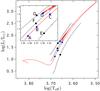 |
Fig. 1 Evolutionary tracks in the Hertzprung-Russel diagram of our models. Selected models are represented by dots. Blue dots correspond to models of a 1.5 M⊙ star at different ages (on the red-giant branch and in the clump). Black dots corresponds to models with the same number of mixed modes over a large separation. |
Global parameters of our models.
2.2. Non-adiabatic computations
To compute theoretical mode frequencies (ν), mode inertias (I), and mode lifetimes (τ), we use the non-adiabatic pulsation code MAD (Dupret et al. 2002). Since the major outcome of non-adiabatic computations are the mode lifetimes (or equivalently damping rates η), we describe the different contributions to the damping and the way they are modelled. The lifetime of a mode, τ, is related to the linewidth Γ of the peak in the power spectrum by  (1)The damping rate of a mode is given by the integral expression (e.g. Dupret et al. 2009)
  (2)where ∫VdW is the work performed by the gas during one oscillation cycle, ξr the radial component of the eigendisplacement vector, R and M the total radius and mass of the star, and I the dimensionless mode inertia.
Two regions of the red giants can play a significant role in the work integral: the radiative region in the core of the red giant and especially around the bottom of the H-burning shell (Wc) and the outer non-adiabatic part of the convective envelope (We)  (3)For more insight into the radiative term, it is useful to consider the asymptotic formulation developed by Dziembowski (1977) (see also Van Hoolst et al. 1998; Godart et al. 2009) for g modes. It gives
 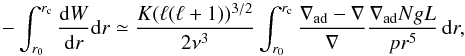 (4)where r0 and rc are the lower and upper radii of the g-cavity, K is a normalisation constant, ∇ and ∇ad are the real and adiabatic gradients, N the Brunt-Väisälä frequency, g the gravity, L the local luminosity, and p the pressure. This formulation shows that the main contribution to the radiative damping occurs around the bottom of the H-burning shell. When the star evolves on the red-giant branch, N/r5 increases as a result of the contraction of the central layers, leading to an increase in the radiative damping as shown in Fig. 2.
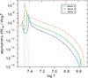 |
Fig. 2 Integrant of the asymptotic expansion of the radiative damping (Eq. (4)) for Models A (blue), B (green), and C (red). The vertical lines represent the lower limit of the H-burning shell in each model. The work is normalised by GM2/R. |
About the convective contribution, we note that the transition region occurs in the upper part of the convective envelope. In this region, the time scale of most energetic turbulent eddies is also close to the oscillation periods. It is therefore important for the estimate of the damping rates to take the interaction between convection and oscillations into account. This is done by using a non-local, time-dependent treatment of the convection (TDC) that considers the variations in the convective flux and of the turbulent pressure due to the oscillations (see Grigahcène et al. 2005; Dupret et al. 2006b, for the description of this treatment). Gough (1977) proposed a second treatment based on the “kinetic of gas” picture of the MLT. For the non-local parameters, we used a = 10 and b = 3 according to the definition of Balmforth (1992). This set of parameters fits the turbulent pressure in sub-adiabatic atmospheric layers of a solar hydrodynamic simulation (Dupret et al. 2006a).
The main source of uncertainty in the TDC treatment comes from the closure term of the perturbed energy equation. This uncertainty appears in the form of a complex parameter β (Eqs. (2) and (33) of Grigahcène et al. 2005). Belkacem et al. (2012) show that this parameter can be adjusted to obtain a plateau of the damping rates at the frequency νmax predicted by the scaling relations ( , first conjectured by Brown et al. 1991), which is similar to having a minimum in the product of the inertia and the damping rate. The existence of this plateau is well known in the solar case and is at the origin of the maximum observed in power spectra. We thus adjust this parameter following the procedure of Belkacem et al. (2012), while paying particular attention to avoiding non-physical spurious oscillations (Grigahcène et al. 2005). In this procedure we assume that the canonical scaling relation for νmax is valid. However, we know this relation is incomplete because, for example, the dependence on the Mach number is missing. Nevertheless, for red-giant stars, the dependence of νmax on the surface gravity dominates, making the variation in the Mach number disappear during the evolution on the red-giant branch (see Belkacem et al. 2013). In Fig. 3, using a unique value of β (βRGB = −0.106−0.945i), we see that we can reproduce a minimum of ηI around the frequency νmax predicted by the scaling relation for all our RGB models. For the helium-burning model, we have to take another value of β (βRC = −0.130−0.950i). This can seem to amount to only a small difference, but our predictions are very sensitive to this parameter. We discuss the effect of this parameter on the lifetimes of the modes in Sect. 3.2. We emphasise that such an approach makes our predictions more accurate than in Dupret et al. (2009), where the bell shape of the heights and the νmax scaling relation were not reproduced.
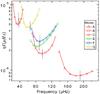 |
Fig. 3 Product of the damping rates (η in μHz) by the dimensionless mode inertia (I) for radial modes for all our RGB models. The minimums of the curves correspond to the frequency of maximum height found in theoretical power spectra. The dashed lines are the νmax deriving from scaling relations. |
A numerical difficulty occurring when computing red giant oscillation spectra comes from the existence of discontinuities of chemical composition and density in the equilibrium models. These discontinuities come from the evolution of the convective zones in the star, and they play an important role in mixed-mode trapping. The amplitudes of eigenfunctions on each side of the discontinuities strongly change from one mode to the next. Therefore, we have adjusted the oscillation code to ensure the continuity of the Lagrangian perturbations of pressure, gravitational potential, and its gradient (see also Reese et al. 2014). Special care was also given to computing the Brunt-Väisälä frequency because it affects our results strongly
Another significant difficulty arises from the high density of non-radial modes over a large separation. It leads to having modes with very close angular frequencies (real part of modes eigenvalues) but with very different damping rates (imaginary part of the eigenvalues). The algorithm solving the non-adiabatic equations searches the eigenvalues by the inverse iteration method. Thus, it converges towards the closest eigenvalue to the initial guess in the complex plane. This eigenvalue is not necessarily the one that corresponds to the frequency and trapping of the initial adiabatic mode. Using only the adiabatic frequencies as an initial guess for the real part of the eigenvalues, the convergence to the correct mode (i.e. the one with the frequency and trapping corresponding to the adiabatic case) of the algorithm is not easily ensured. Initial adiabatic frequencies of different modes could lead to the same eigenvalue in the non-adiabatic algorithm. As a remedy, we have to find an initial guess of the imaginary part for the frequency to be sure to obtain all the modes with different trappings. To do this, we use the inertia ratio between radial and non-radial modes derived from previous adiabatic calculations. We scale the initial guess for the imaginary part of the eigenvalues to the damping rates of radial modes with this inertia ratio.
2.3. Stochastic excitation model
To compute mode heights, one also needs to compute mode driving. For this purpose, we consider the stochastic excitation model of Samadi & Goupil (2001; see also Belkacem et al. 2006a,b; Samadi 2011) and consider the turbulent Reynolds stresses (hereafter PR) as the dominant driving source. We do not take the entropy contribution into account (thermal source of driving) for which a severe deficiency in the modelling with non-adiabatic eigenfunctions appears (as discussed in Samadi et al. 2013).
We use solar parameters for describing the turbulence in the upper convective layers (constrained with a 3D numerical simulation by Samadi et al. 2003) with an extended Kolmogorov spectrum (EKS) for the k dependency of the kinetic energy spectrum (k is the wavenumber in the Fourrier space of turbulence) and a Lorentzian profile, with a high frequency cut-off to take the sweeping phenomena into account for the eddy time-correlation function (Belkacem et al. 2010). For the injection length scale, we assume that it scales as the pressure scale height at the photosphere (Samadi et al. 2008).
With the power provided by the Reynold stresses and the damping rates from non-adiabatic computations, we then compute the amplitude velocity (V) of the mode, using  (5)One can convert the amplitude velocity into bolometric intensity following Samadi et al. (2013). A bolometric conversion that consider the instrumental response was originally proposed by Michel et al. (2009). However, this approach is made in the adiabatic hypothesis. To make direct comparisons with observations, the visibilities of the mode should also be accounted for. We give in Table 2 the conversion factor to obtain the height for the radial mode at νmax in ppm2/μHz. When the non-adiabatic phase lag is neglected here, it is obtained using the relation
  (6)with fT = | δTeff/Teff | / | ξr/R |. We decided to present our results in radial velocity because the conversion to bolometric intensity introduces additional uncertainties.
Conversion factor  from radial velocities to intensity variations for heights around νmax.
To compute the height H of a mode, we have to distinguish between resolved and unresolved modes. We assume that modes are resolved when their lifetimes (τ) are shorter than the duration of observation (Tobs), i.e., τ ≪ Tobs/ 2. In this case, we use for the height of the modes in the power spectra (e.g. Lochard et al. 2005)  (7)and for unresolved modes τ ≫ Tobs/ 2
 (8)where V(R) is the amplitude of the oscillation where it is measured (assumed here at the optical depth τR = 0.1), not including the disk integration factor. These formulae are strictly correct in the limit cases, when the lifetimes are much longer or shorter than the duration of observations. Both formulae give the same value for the height in τ = Tobs/ 2, but using Eq. (7) for τ<Tobs/ 2 and Eq. (8) for τ>Tobs/ 2, as done in Dupret et al. (2009), gives a derivative discontinuity in Tobs/ 2.
The relation between amplitudes and heights depends on whether we deal with a two-sided or a single-sided power spectrum. In the first case, the normalisation is such that the integral of the spectrum from −∞ to + ∞ gives the total energy, so we have  (9)In the opposite case, with a single-sided power spectrum we have
  (10)Here we consider a two-sided power spectrum, which is a different convention than the one used in Chaplin et al. (2009a). Based on the formulation proposed by Fletcher et al. (2006; see also Chaplin et al. 2009a) we have
  (11)which tends to the same value of Eqs. (7) and (8) when τ ≪ Tobs/ 2 and τ ≫ Tobs/ 2, respectively, and interpolate the heights smoothly between these two extreme cases. All our power spectra are computed using this latest description of the height.
With Eq. (11) the height of the mode is only half its maximal height if τ = Tobs/ 2. More observational times is required to fully resolve a mode. Indeed, in an observed power spectrum it is necessary to have many more than two points within a linewidth to resolve the mode.
In this work we choose to take Tobs = 360 days. Even though we now have a longer observational time with Kepler, we picked up this value to discuss the different patterns that can occur in a power spectra and to make a clear distinction between resolved and unresolved modes in all our models. We discuss the effect of increasing Tobs for each model in Sect. 3.
3. Results
3.1. Non-adiabatic effects on power spectra
The shape of the power spectra is mainly determined by two contributions: the modulation of inertia through mode trapping and the radiative damping. To discuss this shape, we describe the behaviour of the ratio between the height of a g-type mode (Hg) and of a p-type mode (Hp). From Eqs. (5) and (11), we have  (12)where fg,p = (Tobsηg,p + 2)-1. In the following, we derive this height ratio in the two asymptotic cases to discuss the main physical properties of the modes that can affect this ratio.
The following simple formulae illustrate this and can help with interpreting our results. Assuming that the modes are resolved, fg/fp in Eq. (12) tends to ηp/ηg and the height ratio is given by  (13)where PRI does not depend on the trapping (see Samadi & Goupil 2001) because the stochastic excitation is only efficient close to the surface (so (PrI)g ≃ (PrI)p). Taking into account the equation of the damping rate Eq. (2) and the decomposition of the work integral into the contribution of the core (Wc) and the envelope (We) Eq. (3), we can rewrite the height ratio as
 ![Mathematical equation: \begin{equation} \label{eq:HgHP_r2} \left(\frac{H_g}{H_p}\right)_{\rm res} \simeq \left(\frac{\left(\eta I\right)_p}{\left(\eta I\right)_g}\right)^2 \simeq \left( \frac{\left(\int{{\rm d}W}\right)_p}{\left(\int{{\rm d}W}\right)_g} \right)^2 \simeq \left(1+\left[\frac{ W_{\rm c} }{W_{\rm e}}\right]_g\right)^{-2} , \end{equation}](/articles/aa/full_html/2014/12/aa23827-14/aa23827-14-eq103.png) (14)where we use (We)g ≃ (We)p since the eigenfunctions of p-type and g-type modes are very close in the envelope. We also neglect the core contribution in the work integral of a p-type mode. We note from this formula that, when the radiative damping of g-type modes is negligible by comparison with the convective damping, their heights are the same as the height of p-type modes if they are resolved. Increasing the radiative damping clearly decreases the height ratio.
(14)where we use (We)g ≃ (We)p since the eigenfunctions of p-type and g-type modes are very close in the envelope. We also neglect the core contribution in the work integral of a p-type mode. We note from this formula that, when the radiative damping of g-type modes is negligible by comparison with the convective damping, their heights are the same as the height of p-type modes if they are resolved. Increasing the radiative damping clearly decreases the height ratio.
If we assume now that the p-type mode is resolved and the g-type mode is not (which is often the case in observed power spectra), the situation is different, and fg/fp in Eq. (12) tends to ηpTobs/ 2 so 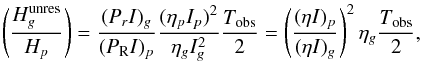 (15)following the same development as in Eq. (14), we find
 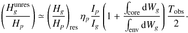 (16)We see from this formula that the height ratio of unresolved modes depends on both their inertia and radiative damping.
We can also rewrite the resolution criteria (Tobs/ 2 >τg) where τg = 1 /ηg represents the lifetime of the mixed mode with the maximum inertia, so that all modes are resolved: 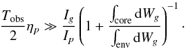 (17)We see in Eqs. (14), (16), and (17) that there are clearly two contributions, the inertia and the non-adiabatic effects, that determine the shape of the power spectra. How the inertia depends on the models is explained in several other studies (e.g. Montalbán & Noels 2013) and can be understood through simple asymptotic derivations (see Goupil et al. 2013, and Appendix A). The work due to non-adiabatic effects for p-type mode can be estimated with scaling relations (Belkacem et al. 2013). The only remaining unknown is the ratio of the work integrals. We discuss its evolution along with the evolution of the star in the next section.
3.2. Power spectrum evolution of a 1.5 M⊙ star
In this section, we discuss the changes in the power spectrum along with the stellar evolution. We focus on the changes in the damping rates and on the height of mixed modes, as well as the effect of increasing the duration of observation. We consider the 1.5 M⊙ models as described in Sect. 2.1.
The theoretical lifetimes of the p-type modes can be strongly affected by the choice of the complex parameter β in the time-dependent convection treatment. We present in Fig. 5 the lifetimes of the radial modes for the model B for different values of the β parameter. All the presented values of β give a minimum of ηI around the frequency νmax predicted by the scaling relation.
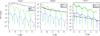 |
Fig. 4 Core and envelope contributions to the work integral for the three RGB models of 1.5 M⊙. The work is normalised by GM2/R. Unlike the envelope contribution, the core contribution depends on the trapping and on the angular degree of the mode. |
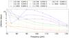 |
Fig. 5 Theoretical lifetimes of radial modes of model B for different values of β. The lifetimes corresponding to β used in this paper are denoted by red squares. |
We first computed the lifetimes of radial modes for many values of β throughout the complex plane. Based on this investigation, we located a value of β that gives a minimum of ηI at νmax for all our RGB models. We first present the results for this β. The power spectra for other values of β are presented at the end of this section.
The work integrals of Models A to C are presented in Fig. 4, while the corresponding mode lifetimes and theoretical power spectra are displayed in Fig. 7. As an overall tendency, we find the well known global changes of the power spectra in Fig. 6 with the evolution of the star on the RGB. (The frequency range of solar-like oscillations goes to lower frequency and, the high frequency and the period spacing decrease, and the height of the modes in the power spectrum increases.) In particular, we find an increase in the heights in the power spectra during the evolution of the star that is qualitatively compatible with previous theoretical computations (Samadi et al. 2012) and with observations (Mosser et al. 2012a).
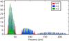 |
Fig. 6 Power spectra of the three RGB models (A, B, and C from right to left) of 1.5 M⊙, summarising the gobal evolutionary tendencies on power spectra. |
For all our models, we show the lifetimes (Figs. 7 and 10 left panel) for the radial and non-radial modes around νmax and the associated power spectra in Figs. 7 and 10 (right panel). These synthetic power spectra take the resolution of the modes for the height of the peaks into account. However, we do not consider the noise background (which can limit the detectability of mixed modes). We therefore consider that the detectability of mixed modes can be derived from the appearance of peaks in our synthetic power spectra. For convenience, we model all peaks by Lorentzians, which give us a limit power spectrum.
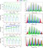 |
Fig. 7 Left: lifetimes of ℓ = 0 (red), ℓ = 1 (blue), and ℓ = 2 (green) modes in Models A, B, C, and D (from top panel to bottom). The dashed line represents Tobs/ 2. Right: corresponding power spectra. The heights in power spectra are given in (m/s)2/μHz. For the sake of simplicity, all peaks are modelled by a Lorentzian, and we did not account for the different mode visibilities that depend on the angular degree. The resolution criteria (and so the time of observation) is taken into account for the height of the modes. |
Model A:
at the bottom of the red-giant branch, the radiative contribution in the work integral (Eq. (3)) is small for all modes in comparison with the convective one (Fig. 4, left panel). In addition, the convective work is a smooth function of the frequency and thus, as already pointed out in Sect. 2.2, is independent of the mode trapping. In the damping rate equation (see Eq. (2)), as a result, only the inertia is responsible for the observed modulation of dipole and quadrupole modes lifetimes (Fig. 7, first panel).
In this model, all dipole mixed modes are resolved (except for low frequencies) and have amplitudes that are high enough to be detected. Since the radiative damping is always negligible, their heights are close to those of the modes trapped in the envelope (p-dominated and radial modes, see Eq. (14)). This spectrum is more regular than the one corresponding to Model A in Dupret et al. (2009). Some quadrupole mixed modes, close to the p-dominated ones, are also visible in the synthetic power spectrum (Fig. 7, first panel).
Increasing the duration would not change the dipole mode profiles. Indeed, since those modes are resolved, their heights no longer depend on the duration of the observations. Thus, at this early stage on the red-giant branch, we already find a clear structure in the power spectrum for dipole modes, allowing us to derive a period spacing. Conversely, as the observation duration increases, the number of visible quadrupole modes increases, too. With four years of observation, some quadrupole modes are resolved (more precisely quadrupole modes with lifetimes lower than 700 days) with heights comparable to the p-dominated modes. Moreover, the height of some quadrupole unresolved modes increases so as to become visible in the synthetic power spectra. Finally, a very long time of observation (typically about 27.5 yrs) is required to have all quadrupole modes resolved, with all heights similar to the heights of the radial ones.
In this star, we also check the behaviour of the ℓ = 3 modes (not represented in the figures). At this early stage on the RGB, they already undergo a strong radiative damping so that only the modes trapped in the envelope are visible in the power spectrum (observations longer than a hundred years would be required to see them). The increase in the radiative damping during the ascension of the red giant branch will prevent detecting ℓ = 3g-types modes higher on the RGB even more. We thus predict that the detectable ℓ = 3 modes in red giants are all p-type modes.
Model B:
higher on the red-giant branch, the radiative contribution to the work integral is similar to the convective contribution for quadrupole modes (Fig. 4). This explains why the lifetimes for low-frequency quadrupole modes level off (Fig. 7, second panel). Moreover, the coupling between the two cavities decreases due to the contraction of the core and the expansion of the envelope. Indeed, when the star evolves, the number of mixed modes by large separation increase, leading to an increase in the inertia ratio between a p-type and a g-type mode (see Appendix A). Because of these two effects, ℓ = 2 mixed modes are no longer visible in our synthetic power spectrum. Even when increasing the duration of observation above two times the lifetime of quadrupole modes (corresponding to approximately 10 years of observation), they would still not be detectable due to their significant radiative damping in the core.
For dipole modes, the convective contribution is still the dominant part of the work integral so that their lifetimes are still clearly modulated by the inertia. Dipole modes strongly trapped in the core are not resolved and have smaller amplitudes. Moreover, as shown in Fig. 7 (second panel), their detection would be made difficult by the overlapping with radial modes and p-type quadrupole modes that exhibit large linewidths. At the end of this section, we detail the effect of the TDC parameter β on the lifetimes of the p-type modes (see also Fig. 5). Other values of this parameter could lead to longer lifetimes, hence to narrower peaks (see Fig. 8). Nevertheless, increasing the duration of observations will increase the heights of dipole modes. Taking four years of observation would allow us to have almost all ℓ = 1 modes resolved, and in this case, their heights are very similar to the p-dominated non-radial modes.
Model C:
for a more evolved model, the radiative damping continues to increase and the coupling between the two cavities becomes very small owing to the expansion of the envelope and contraction of the core. This implies that the lifetimes of all modes, except modes strongly trapped in the envelope, are dominated by the radiative damping (Fig. 7, third panel). This damping is high enough to obtain lifetimes of g-dominated quadrupole mixed modes that are lower than the dipole ones. Consequently, only p-dominated modes are detectable (Fig. 7, third panel). In this model, increasing the duration of the observation even more (even with Tobs> 2τ for all modes) does not lead to detectable mixed modes, because of strong radiative damping (much more important than the convective one, Fig. 4).
Model D:
further along in the evolution, after the helium flash, the star begins to burn helium in its core. This model presents lifetimes similar to those of Model B (Fig. 7, fourth panel). After the helium flash, the core has expanded and the envelope contracted leading to a decrease in the radiative damping of mixed modes and a stronger coupling between the p and g cavities. The appearance of a convective core also contributes to this decrease. The detectability of mixed modes (Fig. 7, fourth panel) is very similar to the case of Model B. After the He flash, the radiative damping of the ℓ = 3 modes is still too high to see the g-type modes in our synthetic power spectrum.
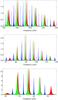 |
Fig. 8 From top to bottom: power spectra of models A, B, and C with new values of the β parameter allowing longer lifetimes for the p-type modes (βA = 1.700−0.700i, βB = −1.940−0.800, βC = −1.780−0.920i). The detectability of the g-type modes is not significantly affected by the change in this parameter. |
Change in β parameter:
with the value of β presented above (the same for all the RGB models), the resulting lifetimes seem shorter than observations (see e.g. Baudin et al. 2011; Appourchaux et al. 2012). We present the power spectra obtained for other values of the β parameter in Fig. 8. In this case, we obtain longer lifetimes but at the price of changing the value of β between each model to be able to reproduce the scaling relation for νmax. This change in parameter does not affect the general aspect of the power spectra much and, in particular, the detectability of g-type modes. Comparing the predicted lifetimes for stellar models fitting a selection of stars to observations would allow us to derive a better constraint for the β parameter.
3.3. A proxy to the shape of power spectra
In the previous section, we have seen that when the stars climb the red-giant branch, the mixed modes become more difficult to detect until their heights are too low to be visible in our synthetic power spectra (even if we consider enough time of observation to resolve all modes). In the following lines, we denote ng and np as the number of nodes of a dipole mode in the g- and p-cavities, respectively. Our analysis of models with the same number of mixed modes over a large separation (Models E to G in Table 1) or, equivalently, a given ratio ng/np shows that they all exhibit the same behaviour for the lifetimes (Fig. 10, left panel). They also present very similar power spectra (Fig. 10, right panel) with the same height ratios of mixed modes. Using the heights computed in the previous sections (i.e. from the calculations of the damping rates and of the Reynold stress), we show in Fig. 9 a relation between the height ratio of g- and p-type modes around νmax on the one side and ng/np on the other side, for fully resolved and partially resolved modes. This relation is particularly marked in the case of fully resolved modes. More computations for a larger number of models will be needed to derive a more precise relation for the relative heights of the modes.
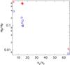 |
Fig. 9 Height ratio between a g-type (the ℓ = 1 with the highest inertia close to νmax) mode and a p-type mode around νmax as a function of ng/np for all our models. Red crosses represent the ideal case where all the modes are resolved. Blue squares are for observation durations of one year. |
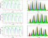 |
Fig. 10 Left: lifetimes of ℓ = 0 (red), ℓ = 1 (blue) and l = 2 (green) modes in models E, F, and G (from top panel to bottom). The dashed line represents Tobs/ 2. Right: corresponding power spectra. The heights in power spectra are given in (m/s)2/μHz. |
We notice that for unresolved modes, the inertia ratio can also be expressed as a function of ng/np (see Appendix A) so that this ratio is a good proxy for the shape of power spectra. In Fig. 9, there is a higher dispersion between the models with the same ng/np with only one year for the duration of observations, because these modes are only partially resolved. We notice that a theoretical evaluation of this proxy is very easy through asymptotic relations and the scaling relation for νmax: 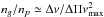 . Taking then the background noise into account, it becomes possible to estimate the detectability of mixed modes along the red-giant branch.
Using this relation, we present in Fig. 11 a curve that corresponds to ng/np ≃ 60, which appears to be the level on the red-giant branch where we are no longer able to see any dipole mixed modes in the synthetic power spectra even by increasing the time of observation to more than ten years (so that all modes are resolved).
4. Conclusion
We have determined lifetimes and heights of radial and non-radial mixed modes for several red-giant models of various evolutionary states and various masses. The corresponding synthetic power spectra agree overall with the observed bell shape. We followed the change in the frequency of maximal amplitude and reproduced the increase in the maximum height along with the evolution of the star. For some of our models, we predicted that long enough observations would increase the heights of mixed modes up to those of radial modes. But for models with a higher density contrast between the core and the envelope, radiative damping becomes too strong and the coupling too weak to have detectable mixed modes in our synthetic power spectra.
In a 1.5 M⊙ star, we predict no detection of dipole mixed modes at νmax ≲ 50 μHz and Δν ≲ 4.9 μHz (corresponding to ng/np ≳ 60) and no detection of quadrupole mixed modes around νmax ≲ 97 μHz and Δν ≲ 8.4 μHz (corresponding to (ng/np)ℓ = 2 ≳ 15). We present in Appendix B a brief qualitative comparison between the tendencies we found in our synthetic power spectra and Kepler spectra. Theoretical power spectra are in qualitatively good agreement with observed ones. The general aspects of mixed-mode spectra and their evolution on the red-giant branch was reproduced well. The lifetimes of our p-type modes seems to be underestimated, but they strongly depend on the complex parameter β (see Sect. 3.2 for more details). Quantitative comparisons between theory and observations will then require a much more precise determination of this parameter.
Computations of power spectra for other masses show that we have very similar lifetimes patterns and power spectra and, in particular, the same height ratios for mixed modes, if we take models with the same number of mixed modes in a large separation. We can then rely on the number of mixed modes by large separation to predict the height ratio between a p-type and a g-type mixed mode for various stars.
More numerical computations that vary not only the mass but also the other parameters of the equilibrium models (e.g. chemical composition or convection treatment) will help to verify these results for a larger set of stars.
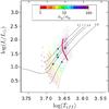 |
Fig. 11 Evolutionary tracks in the HR diagram of all our red-giant branch models. Numbers on the top of the tracks indicate the mass of the star (in M⊙). The color scale indicates models with the same number of mixed modes by large separation. The red line represents the detectability limit we have found for the dipole modes (assuming that all modes are fully resolved). |
Then we will have to compare our height ratios and their dependence with the number of mixed modes by large separations with a large set of observed power spectra (see e.g. Mosser et al. 2012a). In such a large set of observations, some power spectra show depressed mixed modes. Up to now, from a theoretical point of view, we did not find any depressed mixed mode in all our red-giant branch models. The discovery of models for which the inertia of p-type dipole modes, as well as their damping rates, is close to the g-type modes ones could give us more insight into the mechanism depressing these modes, but we did not find such models.
Our results should also be tested by comparing the observed height and lifetimes with the theoretical ones for some individual stars. Such comparisons can now be done with the measurements of linewidths and heights of the modes in solar-like stars (see e.g. Appourchaux et al. 2014), in subgiants (see e.g. Benomar et al. 2013), and in red giants (Huber et al. 2010; Hekker et al. 2010; Corsaro et al. 2012). These comparisons will help in particular to test our TDC treatment and to calibrate the β parameter. This will be the subject of a future work.
Online material
Appendix A: Inertia ratios
For a better understanding of the inertia ratios between a p-type and a g-type mode, we follow the development of Goupil et al. (2013) based on the asymptotic method developed by Shibahashi (1979).
In the asymptotic regime and neglecting the size of the evanescent zone, Goupil et al. (2013) show that the inertia in the envelope of the stars varies as Ienv ≃ (c2/ 2πν)τp and in the core as Icore ≃ (a2/ 2πν)τg, so we can express the total inertia as 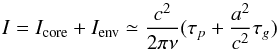 (A.1)with
 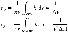 with kr the radial wavenumber and ν the frequency of the mode in μHz. Here, c is a normalisation constant, and a is related to c by (Eqs. (16.49) and (16.50) from Unno et al. 1989) :
 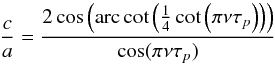 (A.2)where (c/a)2 is a function of ν of period 1 /τp = Δν which varies between 4 (p-modes) and 1/4 (g-modes). Finally when
comparing the inertia of a mode trapped in the envelope (Ip) and of a mode trapped in the core (Ig), we have 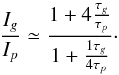 (A.3)This inertia ratio is then a function of the ratio τg/τp = ng/np, the number of mixed-modes by large separation.
Appendix B: Qualitative comparison to Kepler spectra
We present in Fig. B.1 some power spectra obtained with Kepler along with our 1.5 M⊙ RGB theoretical power spectra to show the main tendencies discussed in this paper. Concerning the height ratios and the limit for the detectability of mixed modes in our theoretical power spectra, we found the same tendencies in the observed ones. At the beginning of the red-giant branch, dipole mixed modes have heights that are comparable to p-type modes. Higher on the RGB, dipole mixed modes are partially resolved, and their heights present a clear modulation compared to the heights of p-type modes. At the level of model C, only the p-type modes have significant heights. There are more visible mixed modes in the observed spectra, owing to the presence of rotational multiplets, but without any consequence for their height and width.
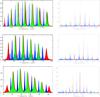 |
Fig. B.1 Theoretical and observed power spectra of Kepler stars with similar masses (from top to bottom: 1.44, 1.48, 1.47 M⊙), Δν, and νmax. The heights in theoretical power spectra are in (m/s)2/μHz. The heights for observed spectra are given in ppm2/μHz divided by a factor 6000 to have scales similar to the theoretical spectra. |
Acknowledgments
This work is financially supported by a doctoral fellowship from the F.R.I.A.
References
- Alexander, D. R., & Ferguson, J. W. 1994, ApJ, 437, 879 [NASA ADS] [CrossRef] [Google Scholar]
- Angulo, C., Arnould, M., Rayet, M., et al. 1999, Nucl. Phys. A, 656, 3 [NASA ADS] [CrossRef] [Google Scholar]
- Appourchaux, T., Benomar, O., Gruberbauer, M., et al. 2012, A&A, 537, A134 [NASA ADS] [CrossRef] [EDP Sciences] [Google Scholar]
- Appourchaux, T., Antia, H. M., Benomar, O., et al. 2014, A&A, 566, A20 [NASA ADS] [CrossRef] [EDP Sciences] [Google Scholar]
- Baglin, A., Michel, E., Auvergne, M., & COROT Team. 2006, in Proc. SOHO 18/GONG 2006/HELAS I, Beyond the spherical Sun, ESA SP, 624 [Google Scholar]
- Balmforth, N. J. 1992, MNRAS, 255, 603 [NASA ADS] [CrossRef] [Google Scholar]
- Baudin, F., Barban, C., Belkacem, K., et al. 2011, A&A, 529, A84 [NASA ADS] [CrossRef] [EDP Sciences] [Google Scholar]
- Beck, P. G., Bedding, T. R., Mosser, B., et al. 2011, Science, 332, 205 [NASA ADS] [CrossRef] [PubMed] [Google Scholar]
- Beck, P. G., Montalban, J., Kallinger, T., et al. 2012, Nature, 481, 55 [NASA ADS] [CrossRef] [Google Scholar]
- Bedding, T. 2011, AGU Fall Meeting Abstracts, F5 [Google Scholar]
- Belkacem, K. 2012, in SF2A-2012: Proc. of the Annual meeting of the French Society of Astronomy and Astrophysics, eds. S. Boissier, P. de Laverny, N. Nardetto, et al., 173 [Google Scholar]
- Belkacem, K., & Samadi, R. 2013, in Lect. Notes Phys. 865, eds. M. Goupil, K. Belkacem, C. Neiner, F. Lignières, & J. J. Green (Berlin: Springer Verlag), 179 [Google Scholar]
- Belkacem, K., Samadi, R., Goupil, M. J., & Kupka, F. 2006a, A&A, 460, 173 [NASA ADS] [CrossRef] [EDP Sciences] [Google Scholar]
- Belkacem, K., Samadi, R., Goupil, M. J., Kupka, F., & Baudin, F. 2006b, A&A, 460, 183 [NASA ADS] [CrossRef] [EDP Sciences] [Google Scholar]
- Belkacem, K., Samadi, R., Goupil, M. J., et al. 2010, A&A, 522, L2 [NASA ADS] [CrossRef] [EDP Sciences] [Google Scholar]
- Belkacem, K., Goupil, M. J., Dupret, M. A., et al. 2011, A&A, 530, A142 [NASA ADS] [CrossRef] [EDP Sciences] [Google Scholar]
- Belkacem, K., Dupret, M. A., Baudin, F., et al. 2012, A&A, 540, L7 [NASA ADS] [CrossRef] [EDP Sciences] [Google Scholar]
- Belkacem, K., Appourchaux, T., Baudin, F., et al. 2013, in EPJ Web Conf., 43, 3009 [Google Scholar]
- Benomar, O., Bedding, T. R., Mosser, B., et al. 2013, ApJ, 767, 158 [NASA ADS] [CrossRef] [Google Scholar]
- Benomar, O., Belkacem, K., Bedding, T. R., et al. 2014, ApJ, 781, L29 [NASA ADS] [CrossRef] [PubMed] [Google Scholar]
- Böhm-Vitense, E. 1958, Z. Astrophys., 46, 108 [Google Scholar]
- Brown, T. M., Gilliland, R. L., Noyes, R. W., & Ramsey, L. W. 1991, ApJ, 368, 599 [NASA ADS] [CrossRef] [Google Scholar]
- Cassisi, S., Potekhin, A. Y., Pietrinferni, A., Catelan, M., & Salaris, M. 2007, ApJ, 661, 1094 [NASA ADS] [CrossRef] [Google Scholar]
- Chaplin, W. J., Elsworth, Y., Isaak, G. R., et al. 1998, MNRAS, 298, L7 [NASA ADS] [CrossRef] [Google Scholar]
- Chaplin, W. J., Houdek, G., Elsworth, Y., et al. 2009a, ApJ, 692, 531 [NASA ADS] [CrossRef] [Google Scholar]
- Chaplin, W. J., Houdek, G., Karoff, C., Elsworth, Y., & New, R. 2009b, A&A, 500, L21 [NASA ADS] [CrossRef] [EDP Sciences] [Google Scholar]
- Christensen-Dalsgaard, J. 2004, Sol. Phys., 220, 137 [NASA ADS] [CrossRef] [Google Scholar]
- Corsaro, E., Stello, D., Huber, D., et al. 2012, ApJ, 757, 190 [NASA ADS] [CrossRef] [Google Scholar]
- Corsaro, E., Fröhlich, H.-E., Bonanno, A., et al. 2013, MNRAS, 430, 2313 [NASA ADS] [CrossRef] [Google Scholar]
- De Ridder, J., Barban, C., Baudin, F., et al. 2009, Nature, 459, 398 [Google Scholar]
- Deheuvels, S., García, R. A., Chaplin, W. J., et al. 2012, ApJ, 756, 19 [NASA ADS] [CrossRef] [Google Scholar]
- Deheuvels, S., Doğan, G., Goupil, M. J., et al. 2014, A&A, 564, A27 [NASA ADS] [CrossRef] [EDP Sciences] [Google Scholar]
- Dupret, M.-A., De Ridder, J., Neuforge, C., Aerts, C., & Scuflaire, R. 2002, A&A, 385, 563 [NASA ADS] [CrossRef] [EDP Sciences] [Google Scholar]
- Dupret, M.-A., Goupil, M.-J., Samadi, R., Grigahcène, A., & Gabriel, M. 2006a, in Proc. of SOHO 18/GONG 2006/HELAS I, Beyond the spherical Sun, ESA SP, 624 [Google Scholar]
- Dupret, M.-A., Samadi, R., Grigahcene, A., Goupil, M.-J., & Gabriel, M. 2006b, Comm. Asteroseism., 147, 85 [Google Scholar]
- Dupret, M.-A., Belkacem, K., Samadi, R., et al. 2009, A&A, 506, 57 [NASA ADS] [CrossRef] [EDP Sciences] [Google Scholar]
- Dziembowski, W. A. 1971, Acta Astron., 21, 289 [NASA ADS] [Google Scholar]
- Dziembowski, W. 1977, Acta Astron., 27, 95 [NASA ADS] [Google Scholar]
- Dziembowski, W. A. 2012, A&A, 539, A83 [NASA ADS] [CrossRef] [EDP Sciences] [Google Scholar]
- Dziembowski, W. A., Gough, D. O., Houdek, G., & Sienkiewicz, R. 2001, MNRAS, 328, 601 [NASA ADS] [CrossRef] [Google Scholar]
- Eggenberger, P., Montalbán, J., & Miglio, A. 2012, A&A, 544, L4 [NASA ADS] [CrossRef] [EDP Sciences] [Google Scholar]
- Fletcher, S. T., Chaplin, W. J., Elsworth, Y., Schou, J., & Buzasi, D. 2006, MNRAS, 371, 935 [NASA ADS] [CrossRef] [Google Scholar]
- Gilliland, R. L., Jenkins, J. M., Borucki, W. J., et al. 2010, ApJ, 713, L160 [NASA ADS] [CrossRef] [Google Scholar]
- Godart, M., Noels, A., Dupret, M.-A., & Lebreton, Y. 2009, MNRAS, 396, 1833 [NASA ADS] [CrossRef] [Google Scholar]
- Gough, D. O. 1977, ApJ, 214, 196 [NASA ADS] [CrossRef] [Google Scholar]
- Goupil, M. J., Mosser, B., Marques, J. P., et al. 2013, A&A, 549, A75 [NASA ADS] [CrossRef] [EDP Sciences] [Google Scholar]
- Grevesse, N., & Noels, A. 1993, in Perfectionnement de l’Association Vaudoise des Chercheurs en Physique, eds. B. Hauck, S. Paltani, & D. Raboud, 205 [Google Scholar]
- Grigahcène, A., Dupret, M.-A., Gabriel, M., Garrido, R., & Scuflaire, R. 2005, A&A, 434, 1055 [NASA ADS] [CrossRef] [EDP Sciences] [Google Scholar]
- Hekker, S., Barban, C., Baudin, F., et al. 2010, A&A, 520, A60 [NASA ADS] [CrossRef] [EDP Sciences] [Google Scholar]
- Henyey, L., Vardya, M. S., & Bodenheimer, P. 1965, ApJ, 142, 841 [NASA ADS] [CrossRef] [Google Scholar]
- Houdek, G., & Gough, D. O. 2002, MNRAS, 336, L65 [NASA ADS] [CrossRef] [Google Scholar]
- Huber, D., Bedding, T. R., Stello, D., et al. 2010, ApJ, 723, 1607 [NASA ADS] [CrossRef] [Google Scholar]
- Iglesias, C. A., & Rogers, F. J. 1996, ApJ, 464, 943 [NASA ADS] [CrossRef] [Google Scholar]
- Lochard, J., Samadi, R., & Goupil, M. J. 2005, A&A, 438, 939 [NASA ADS] [CrossRef] [EDP Sciences] [Google Scholar]
- Marques, J. P., Goupil, M. J., Lebreton, Y., et al. 2013, A&A, 549, A74 [NASA ADS] [CrossRef] [EDP Sciences] [Google Scholar]
- Michel, E., Samadi, R., Baudin, F., et al. 2009, A&A, 495, 979 [NASA ADS] [CrossRef] [EDP Sciences] [Google Scholar]
- Miglio, A., Montalbán, J., Baudin, F., et al. 2009, A&A, 503, L21 [NASA ADS] [CrossRef] [EDP Sciences] [MathSciNet] [Google Scholar]
- Miglio, A., Chiappini, C., Morel, T., et al. 2013, MNRAS, 429, 423 [NASA ADS] [CrossRef] [Google Scholar]
- Montalbán, J., & Noels, A. 2013, in EPJ Web Conf., 43, 3002 [Google Scholar]
- Montalbán, J., Miglio, A., Noels, A., Scuflaire, R., & Ventura, P. 2010, Astron. Nachr., 331, 1010 [NASA ADS] [CrossRef] [Google Scholar]
- Mosser, B., Belkacem, K., Goupil, M.-J., et al. 2010, A&A, 517, A22 [NASA ADS] [CrossRef] [EDP Sciences] [Google Scholar]
- Mosser, B., Barban, C., Montalbán, J., et al. 2011, A&A, 532, A86 [NASA ADS] [CrossRef] [EDP Sciences] [Google Scholar]
- Mosser, B., Elsworth, Y., Hekker, S., et al. 2012a, A&A, 537, A30 [NASA ADS] [CrossRef] [EDP Sciences] [Google Scholar]
- Mosser, B., Goupil, M. J., Belkacem, K., et al. 2012b, A&A, 548, A10 [NASA ADS] [CrossRef] [EDP Sciences] [Google Scholar]
- Mosser, B., Dziembowski, W. A., Belkacem, K., et al. 2013, A&A, 559, A137 [NASA ADS] [CrossRef] [EDP Sciences] [Google Scholar]
- Ouazzani, R.-M., Goupil, M. J., Dupret, M.-A., & Marques, J. P. 2013, A&A, 554, A80 [NASA ADS] [CrossRef] [EDP Sciences] [Google Scholar]
- Potekhin, A. Y., Baiko, D. A., Haensel, P., & Yakovlev, D. G. 1999, A&A, 346, 345 [NASA ADS] [Google Scholar]
- Reese, D. R., Lara, F. E., & Rieutord, M. 2014, in IAU Symp. 301, eds. J. A. Guzik, W. J. Chaplin, G. Handler, & A. Pigulski, 169 [Google Scholar]
- Rogers, F. J., & Nayfonov, A. 2002, ApJ, 576, 1064 [Google Scholar]
- Samadi, R. 2011, in Lect. Notes Phys. 832, eds. J.-P. Rozelot, & C. Neiner (Berlin: Springer Verlag), 305 [Google Scholar]
- Samadi, R., & Goupil, M.-J. 2001, A&A, 370, 136 [NASA ADS] [CrossRef] [EDP Sciences] [Google Scholar]
- Samadi, R., Nordlund, Å., Stein, R. F., Goupil, M. J., & Roxburgh, I. 2003, A&A, 403, 303 [Google Scholar]
- Samadi, R., Belkacem, K., Goupil, M.-J., Ludwig, H.-G., & Dupret, M.-A. 2008, Commun. Asteroseismol., 157, 130 [NASA ADS] [Google Scholar]
- Samadi, R., Belkacem, K., Dupret, M.-A., et al. 2012, A&A, 543, A120 [NASA ADS] [CrossRef] [EDP Sciences] [Google Scholar]
- Samadi, R., Belkacem, K., Dupret, M.-A., et al. 2013, EPJ Web Conf., 43, 3008 [Google Scholar]
- Saumon, D., Chabrier, G., & van Horn, H. M. 1995, ApJS, 99, 713 [NASA ADS] [CrossRef] [Google Scholar]
- Scuflaire, R. 1974, A&A, 36, 107 [NASA ADS] [Google Scholar]
- Shibahashi, H. 1979, PASJ, 31, 87 [NASA ADS] [Google Scholar]
- Stolzmann, W., & Bloecker, T. 1996, A&A, 314, 1024 [NASA ADS] [Google Scholar]
- Tassoul, M. 1980, ApJS, 43, 469 [NASA ADS] [CrossRef] [Google Scholar]
- Unno, W., Osaki, Y., Ando, H., Saio, H., & Shibahashi, H. 1989, Nonradial oscillations of stars (Tokyo: University of Tokyo Press) [Google Scholar]
- Van Hoolst, T., Dziembowski, W. A., & Kawaler, S. D. 1998, MNRAS, 297, 536 [NASA ADS] [CrossRef] [Google Scholar]
- Ventura, P., D’Antona, F., & Mazzitelli, I. 2008, Ap&SS, 316, 93 [NASA ADS] [CrossRef] [Google Scholar]
All Tables
Conversion factor from radial velocities to intensity variations for heights around νmax.
All Figures
|
Fig. 1 Evolutionary tracks in the Hertzprung-Russel diagram of our models. Selected models are represented by dots. Blue dots correspond to models of a 1.5 M⊙ star at different ages (on the red-giant branch and in the clump). Black dots corresponds to models with the same number of mixed modes over a large separation. |
| In the text | |
|
Fig. 2 Integrant of the asymptotic expansion of the radiative damping (Eq. (4)) for Models A (blue), B (green), and C (red). The vertical lines represent the lower limit of the H-burning shell in each model. The work is normalised by GM2/R. |
| In the text | |
|
Fig. 3 Product of the damping rates (η in μHz) by the dimensionless mode inertia (I) for radial modes for all our RGB models. The minimums of the curves correspond to the frequency of maximum height found in theoretical power spectra. The dashed lines are the νmax deriving from scaling relations. |
| In the text | |
|
Fig. 4 Core and envelope contributions to the work integral for the three RGB models of 1.5 M⊙. The work is normalised by GM2/R. Unlike the envelope contribution, the core contribution depends on the trapping and on the angular degree of the mode. |
| In the text | |
|
Fig. 5 Theoretical lifetimes of radial modes of model B for different values of β. The lifetimes corresponding to β used in this paper are denoted by red squares. |
| In the text | |
|
Fig. 6 Power spectra of the three RGB models (A, B, and C from right to left) of 1.5 M⊙, summarising the gobal evolutionary tendencies on power spectra. |
| In the text | |
|
Fig. 7 Left: lifetimes of ℓ = 0 (red), ℓ = 1 (blue), and ℓ = 2 (green) modes in Models A, B, C, and D (from top panel to bottom). The dashed line represents Tobs/ 2. Right: corresponding power spectra. The heights in power spectra are given in (m/s)2/μHz. For the sake of simplicity, all peaks are modelled by a Lorentzian, and we did not account for the different mode visibilities that depend on the angular degree. The resolution criteria (and so the time of observation) is taken into account for the height of the modes. |
| In the text | |
|
Fig. 8 From top to bottom: power spectra of models A, B, and C with new values of the β parameter allowing longer lifetimes for the p-type modes (βA = 1.700−0.700i, βB = −1.940−0.800, βC = −1.780−0.920i). The detectability of the g-type modes is not significantly affected by the change in this parameter. |
| In the text | |
|
Fig. 9 Height ratio between a g-type (the ℓ = 1 with the highest inertia close to νmax) mode and a p-type mode around νmax as a function of ng/np for all our models. Red crosses represent the ideal case where all the modes are resolved. Blue squares are for observation durations of one year. |
| In the text | |
|
Fig. 10 Left: lifetimes of ℓ = 0 (red), ℓ = 1 (blue) and l = 2 (green) modes in models E, F, and G (from top panel to bottom). The dashed line represents Tobs/ 2. Right: corresponding power spectra. The heights in power spectra are given in (m/s)2/μHz. |
| In the text | |
|
Fig. 11 Evolutionary tracks in the HR diagram of all our red-giant branch models. Numbers on the top of the tracks indicate the mass of the star (in M⊙). The color scale indicates models with the same number of mixed modes by large separation. The red line represents the detectability limit we have found for the dipole modes (assuming that all modes are fully resolved). |
| In the text | |
|
Fig. B.1 Theoretical and observed power spectra of Kepler stars with similar masses (from top to bottom: 1.44, 1.48, 1.47 M⊙), Δν, and νmax. The heights in theoretical power spectra are in (m/s)2/μHz. The heights for observed spectra are given in ppm2/μHz divided by a factor 6000 to have scales similar to the theoretical spectra. |
| In the text | |
Current usage metrics show cumulative count of Article Views (full-text article views including HTML views, PDF and ePub downloads, according to the available data) and Abstracts Views on Vision4Press platform.
Data correspond to usage on the plateform after 2015. The current usage metrics is available 48-96 hours after online publication and is updated daily on week days.
Initial download of the metrics may take a while.