| Issue |
A&A
Volume 572, December 2014
|
|
|---|---|---|
| Article Number | A40 | |
| Number of page(s) | 13 | |
| Section | Extragalactic astronomy | |
| DOI | https://doi.org/10.1051/0004-6361/201423805 | |
| Published online | 26 November 2014 | |
Outflow of hot and cold molecular gas from the obscured secondary nucleus of NGC 3256: closing in on feedback physics⋆,⋆⋆
1 Centro de Astrobiología (INTA-CSIC), Ctra de Torrejón a Ajalvir, km 4, 28850 Torrejón de Ardoz, Madrid, Spain
e-mail: This email address is being protected from spambots. You need JavaScript enabled to view it.
2 Istituto di Astrofisica e Planetologia Spaziali (INAF), Via Fosso del Cavaliere 100, 00133 Roma, Italy
3 Observatorio Astronómico Nacional (OAN), Observatorio de Madrid, Alfonso XII 3, 28014 Madrid, Spain
4 Instituto de Física de Cantabria (CSIC-UC), 39005 Santander, Spain
Received: 13 March 2014
Accepted: 29 August 2014
Abstract
The nuclei of merging galaxies are often deeply buried in dense layers of gas and dust. In these regions, gas outflows driven by starburst and active galactic nuclear activity are believed to play a crucial role in the evolution of these galaxies. However, to fully understand this process it is essential to resolve the morphology and kinematics of such outflows. Using near-infrared integral-field spectroscopy obtained with SINFONI on the Very Large Telescope, we detect a kpc-scale structure of high-velocity molecular hydrogen (H2) gas associated with the deeply buried secondary nucleus of the infrared-luminous merger-galaxy NGC 3256. We show that this structure is most likely the hot component of a molecular outflow, which was recently also detected in the cold molecular gas through CO emission. This outflow, with a total molecular gas mass of MH2 ~ 2 × 10⁷M⊙, is among the first to be spatially resolved in both the hot molecular H2 gas with VLT/SINFONI and the cold molecular CO emitting gas with ALMA. The hot and cold components share a similar morphology and kinematics, with a hot-to-cold molecular gas mass ratio of ~ 6 × 10⁻⁵. The high (~100 pc) resolution at which we map the geometry and velocity structure of the hot outflow reveals a biconical morphology with opening angle ~40° and gas spread across a FWZI ~ 1200 km s-1. Because this collimated outflow is oriented close to the plane of the sky, the molecular gas may reach maximum intrinsic outflow velocities of ~1800 km s-1, with an average mass outflow rate of at least Ṁoutfl ~ 20 M⊙ yr-1. By modeling the line-ratios of various near-infrared H2 transitions, we show that the H2-emitting gas in the outflow is heated through shocks or X-rays to a temperature of T ~ 1900 ± 300 K. The energy needed to drive the collimated outflow is most likely provided by a hidden Compton-thick AGN or by the nuclear starburst. We show that the global kinematics of the molecular outflow that we detect in NGC 3256 mimic those of CO-outflows that have been observed at much lower spatial resolution in starburst- and active galaxies.
Key words: galaxies: individual: NGC 3256 / galaxies: starburst / galaxies: active / galaxies: nuclei / ISM: jets and outflows / dust, extinction
Appendix A is available in electronic form at http://www.aanda.org
The final data products are only available at the CDS via anonymous ftp to cdsarc.u-strasbg.fr (130.79.128.5) or via http://cdsarc.u-strasbg.fr/viz-bin/qcat?J/A+A/572/A40
Marie Curie Fellow.
© ESO, 2014
1. Introduction
Luminous and ultra-luminous infrared galaxies, also called LIRGs (LIR> 1011L⊙) and ULIRGs (LIR> 1012L⊙), are galaxies with massive dust-enshrouded star formation and often a deeply buried active galactic nucleus (AGN; Sanders & Mirabel 1996). Because (U)LIRGs can be found at relatively low z, they are excellent laboratories for studying physical processes that are crucial in the evolution of massive galaxies, from galaxy merging to starburst/AGN-induced feedback. These processes, in particular when they occur in the nuclei, are often hidden behind thick layers of gas and dust, which absorb most of the light before re-radiating it at infrared (IR) wavelengths.
Integral-field spectroscopy in the near-IR provides an excellent tool to study the physical processes in the central regions of (U)LIRGs. At near-IR wavelengths the dust extinction is much lower than in the optical. In addition, in the near-IR a variety of emission lines from different gas phases, as well as stellar absorption lines, can often be observed simultaneously (from coronal [Si VI] and ionized Brγ or Paα to partially ionized [Fe II] and molecular H2 emission). Particularly interesting is that a range of near-IR transitions of H2 can be targeted to study the physical properties of the molecular gas. Another intrinsic advantage of near-IR integral-field spectroscopy is that, apart from being able to image the gas at high spatial resolution, different gas structures can also be distinguished kinematically. This can be done in detail by decomposing complex line profiles into multiple kinematic components across the field of view of the spectrograph.
The strength of a detailed kinematic analysis of near-IR integral-field spectra was recently shown by Rupke & Veilleux (2013), who revealed the base of a deeply buried H2 outflow in the nearby quasi-stellar object QSO F08572+3915. Other observational techniques have also revealed evidence that links nuclear AGN and starburst activity with heating and outflow of neutral and molecular gas in low-z galaxies (Oosterloo et al. 2000; Leon et al. 2007; Feruglio et al. 2010; Alatalo et al. 2011; Rupke & Veilleux 2011; Aalto et al. 2012; Guillard et al. 2012; Dasyra & Combes 2012; Combes et al. 2013; Morganti et al. 2005, 2013a,b; Mahony et al. 2013; Dasyra et al. 2014; Garcia-Burillo et al. 2014; Cazzoli et al. 2014; Tadhunter et al. 2014). Moreover, recent surveys with instruments like Herschel and the Plateau de Bure Interferometer revealed evidence of massive outflows of molecular gas in ULIRGs (e.g., Chung et al. 2011; Sturm et al. 2011; Spoon et al. 2013; Veilleux et al. 2013; Cicone et al. 2014), which complement extensively studied ionized gas outflows in these systems (e.g., Heckman et al. 1990; Westmoquette et al. 2012; Bellocchi et al. 2013; Rodríguez Zaurín et al. 2013; Arribas et al. 2014). Thus, if feedback onto the molecular gas is common in merger systems with dust-obscured starburst/AGN cores, we expect to find evidence of this through detailed 3D kinematic studies of the near-IR H2 lines in other nearby IR-luminous galaxies.
In this paper, we perform a kinematic and morphological analysis of the near-IR H2 emission from molecular gas associated with the deeply buried secondary nucleus of NGC 3256, which is the most luminous LIRG within z< 0.01 (Lir ~ 5 × 10¹¹L⊙; Sanders et al. 2003). In Piqueras López et al. (2012a) we previously revealed that NGC 3256 contains a large-scale rotating H2 disk, which we imaged by tracing the H2 1−0 S(1) λ = 2.12 μm line with near-IR integral-field data from the Spectrograph for Integral Field Observations in the Near Infrared at the Very Large Telescope (VLT/SINFONI; Eisenhauer et al. 2003; Bonnet et al. 2004). However, the standard single-Gaussian fitting procedure that we applied in Piqueras López et al. (2012a) revealed residuals that suggested the presence of more complex kinematics across various regions (see Sect. 2). We further explore the complex kinematics of the H2 gas in NGC 3256 in this paper.
1.1. NGC 3256
NGC 3256 is a gas-rich merger with prominent tidal tails, galactic winds and ionized gas outflows (e.g., Scarrott et al. 1996; Moran et al. 1999; Heckman et al. 2000; Lípari et al. 2000, 2004; English et al. 2010; Monreal-Ibero et al. 2010; Rich et al. 2011; Leitherer et al. 2013; Bellocchi et al. 2013; Arribas et al. 2014). It contains two nuclei, separated by ~1 kpc. The secondary, or southern, nucleus is heavily obscured, as revealed with IR and radio observations (Norris & Forbes 1995; Kotilainen et al. 1996; Alonso-Herrero et al. 2006a; Lira et al. 2008; Díaz-Santos et al. 2008). Various authors have claimed that this secondary nucleus may host a heavily obscured AGN (e.g., Kotilainen et al. 1996; Neff et al. 2003). So far, X-ray studies provided inconclusive evidence for this (Lira et al. 2002; Jenkins et al. 2004; Pereira-Santaella et al. 2011), while the near- and mid-IR properties of both nuclei are ascribed mostly to star-formation activity (Alonso-Herrero et al. 2006b; Lira et al. 2008; Pereira-Santaella et al. 2010; Alonso-Herrero et al. 2012).
Molecular gas was detected through observations of H2 and various tracers of cold molecular gas (e.g., Moorwood & Oliva 1994; Doyon et al. 1994; Sargent et al. 1989; Mirabel et al. 1990; Aalto et al. 1991; Casoli et al. 1992; Baan et al. 2008). Sakamoto et al. (2006) used CO(2−1) observations taken with the Submillimeter Array (SMA) to map a large (r> 3 kpc) disk of cold molecular gas rotating about the mid-point between the two nuclei. Part of this disk was also mapped in H2 (Piqueras López et al. 2012a) and Hα (Lípari et al. 2000; Rodríguez-Zaurín et al. 2011; Bellocchi et al. 2013). Sakamoto et al. (2006) also found a high-velocity component of molecular gas. In a concurrent paper, Sakamoto et al. (2014) present new ALMA data that reveal that the high-velocity molecular gas is associated with two outflows, namely a starburst-driven superwind from the primary nucleus and a much more collimated kpc-scale bipolar outflow from the secondary nucleus. Our VLT/SINONI H2 data reveal independent evidence of this collimated bipolar outflow and will shed a new light on its nature.
Throughout this paper, we assume z = 0.009354 (which is the redshift of the Brγ peak emission at the location of the secondary nucleus) and D = 44.6 Mpc (1′′ = 216 pc), as per Piqueras López et al. (2012a).
2. Data
We use near-IR data obtained with VLT/SINFONI previously presented in Piqueras López et al. (2012a), with pixel-size 0.125′′, seeing ~0.6′′, spectral resolution 6.0±0.6 Å and dispersion 2.45 Å/pixel. These data originally revealed a large-scale H2 disk (Sect. 1), which is also shown in our Fig. 1. From visual inspection, the single Gaussian fit previously applied to the H2 1−0 S(1) emission line by Piqueras López et al. (2012a) did not produce satisfactory results for mapping the full kinematic structure of the hot molecular gas. This was most notable in the regions ~2.5 arcsec south and ~3.5 arcsec north of the secondary nucleus in Piqueras López et al. (2012a), where the measured velocity from the Gaussian fit to the H2 1−0S (1) line did not reflect the otherwise regular rotation pattern of the large-scale H2 disk. For the current work, we modified the data analysis routine used by Piqueras López et al. (2012a) to fit two Gaussian components to the H2 line profile there where required. This routine was compiled for the Interactive Data Language (IDL) and uses the MPFIT package for the χ2 minimization (Markwardt 2009). No constrains were placed on the fitting parameters and all fits were visually inspected to ensure their validity. A flux (F), velocity (v) and velocity dispersion (σ) map (corrected for instrumental broadening) were created for each component, and boxcar-smoothed by 3 pixels in both spatial directions.
We also used archival ALMA cycle-0 data to compare the morphology and kinematics of certain H2 features with those observed in CO(3−2) (program 2011.0.00525; PI K. Sakamoto, see also Sakamoto 2013a,b). These data have a spatial resolution of 1.2′′ × 0.7′′ (PA = 23°) and channel width of 10 km s-1, with the standard ALMA achival pipeline-reduction applied. In a concurrent paper, Sakamoto et al. (2014) present these CO data (and other molecular gas tracers) using additional calibration and analysis techniques, hence we refer to their work for further details on the CO properties of NGC 3256.
Images of the Hubble Space Telescope Near Infrared Camera and Multi-Object Spectrometer 2 (HST/NICMOS2) filters F160W, F212N and F237M (prog. ID 7251, PI: J. Black; see also Rossa et al. 2007) and the Wide Field and Planetary Camera 2 (HST/WFPC2) filter F814W (prog. ID 5369, PI: S. Zepf; see also Zepf et al. 1999; Laine et al. 2003) were extracted through the Hubble Legacy Archive. Our SINFONI data were overlaid onto these HST images by visually matching the coordinates to those of the secondary nucleus in the HST/NICMOS2 data.
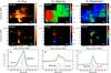 |
Fig. 1 SINFONI view of the H2 emission in NGC 3256, mostly covering the region surrounding the secondary (southern) nucleus. The primary and secondary nucleus are marked with an × and +, respectively, and are shown in more detail in Fig. 3. Top + middle: maps of the H2 flux (F), velocity of the emission-line peak (v) and velocity dispersion (σ = FWHM/ 2.35, with FWHM the full width at half the maximum intensity) of both the narrow- (top) and broad-component gas (middle). Velocities are with respect to z = 0.009354 as per Piqueras López et al. (2012a), which is the assumed systemic velocity of the secondary core (Sect. 1.1). Units are in × 10-17 erg s-1 cm-2 (F) and km s-1 (v and σ). Bottom: H2 emission-line profiles, plus continuum-subtracted 2-component Gaussian fit, in regions A, B and C. The spectra were extracted from a circular aperture of 13 spaxels of 0.125′′ × 0.125′′ each (i.e., roughly the size of the seeing disk), centered on the broad-component H2 features. |
3. Results
3.1. Hot molecular structure
The results of mapping the H2 1−0 S(1) line with two Gaussian components are shown in Fig. 1. A “narrow” component is visible across the field of view (F.o.V.), tracing the large-scale rotating molecular gas disk previously discussed by Piqueras López et al. (2012a). A second, “broad” component is detected in three regions (A, B and C in Fig. 1). Properties of the broad-component emission are given in Table 1.
The most prominent broad-component features are the bright, blue-shifted structure A (projected distance ~440 pc south of the secondary nucleus) and the redshifted structure B (~800 pc north of the secondary nucleus). The integrated intensity is I = 4.2 and 3.8 × 10⁻¹⁵ erg s-1 cm-2 across regions A and B, respectively. This H2 gas has velocities that appear to be decoupled from those of the main narrow-component disk and shows a significantly higher velocity dispersion than the disk emission. When this broad component is integrated across the full extent of regions A+B, it appears to be centered both spatially and kinematically around the secondary nucleus. The corresponding integrated broad-component profile shown in Fig. 2 covers a total full-width-at-zero-intensity velocity range of FWZItot ≈ 1200 km s-1 (or FWHMtot ~ 560 km s-1) and is symmetric with respect to our assumed systemic velocity of the secondary nucleus. We note that our SINFONI F.o.V. does not cover the primary nucleus (north of region B), while the line-fitting south of region A becomes too uncertain (Fig. 1 top-middle), hence the full extent of the broad-component H2 structure may not be revealed.
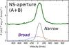 |
Fig. 2 Integrated H2 emission-line profile across the combined 1.1′′ × 8.8′′ north-south aperture that covers the full broad-component A+B region (as visualized in the middle-left panel of Fig. 1). The 0-velocity is defined as the redshift of the Brγ peak-emission at the location of the secondary nucleus. The ~60 km s-1 redshift of the narrow component is likely due to the fact that the kinematic center of the large-scale molecular disk is ~500 pc north of the secondary nucleus. |
 |
Fig. 3 Left: contours of the broad-component H2 emission from Fig. 1 (levels: 0.7, 1.3, 2.0, 2.8, 4.0 × 10⁻¹⁷ erg s-1 cm-2) overlaid onto an optical image taken with the HST/WFPC2 F814W724−878 nm wide-band filter. Middle: contours of the broad-component H2 emission overlaid onto a 3-color near-IR image of the same region taken with the HST/NICMOS2 (filters: blue = F160W1.4−1.8 μm, green = F212N2.111−2.132 μm, red = F237M2.29−2.44 μm). Top right: VLT/SINFONI spectrum obtained against the region of peak H2 emission in region A (aperture 13 pixels). Visualized are the regions of the HST/NICMOS F212N narrow-band (2.111−2.132 μm) and F237M medium-band filter (2.29−2.44 μm). The F237M filter includes the prominent H2 1−0 Q(1) and Q(2) lines. The F160W wide-band filter (1.4−1.8 μm) covers the VLT/SINFONI H-band spectrum of this object, with [Fe II] as the most prominent emission-line in this spectral region (see Piqueras López et al. 2012a). Right bottom: region A as observed in the three different NICMOS filters. The arrows point to the region with enhanced H2 emission in both the VLA/SINFONI and HST/NICMOS F237M data. |
Physical parameters of the broad-component H2 1-0S(1) features.
Figure 3 shows a contour map of the broad-component H2 emission overlaid onto various optical and near-IR HST images. The 3-color composite HST/NICMOS F160W+H212N+F237M image in Fig. 3 (middle) shows a distinctive red feature at the location of the bright H2 emission in region A. As shown on the right of Fig. 3, this red feature (marked with an arrow) only appears in the NICMOS F237M filter. The F237M filter (2.29−2.44 μm) includes the H2 1−0Q(1), 1−0Q(2) and 1−0Q(3) emission lines at the redshift of NGC 3256, of which the prominent Q(1) and Q(2) lines fall within the wavelength range of our SINFONI data1. The same red feature does not appears in the F160W and F212N filters that mostly trace the near-IR continuum. We thus believe that the red feature south of the secondary nucleus in the NICMOS image consists of molecular line emission, which we also see as enhanced H2 emission in both the narrow and broad component in region A (Fig. 1). No obvious features are visible in any of the NICMOS filters in region B. We also find no obvious stellar or dusty counterpart that follows the broad-component H2 emission across regions A and B in optical wide-band HST/WFPC2 imaging (Fig. 3 - left), although a dark line does appear to cross the region of peak H2 brightness (at least in projection). In addition, the Brγ-line of ionized gas in our SINFONI data is very weak in region A and does not have a prominent broad component in region B. It should be noted that the weak Brγ does appear to have an increased velocity dispersion in region A (Piqueras López et al. 2012a), while a weak broad-component feature in Hα has been reported south of region A by Bellocchi et al. (2013). Nevertheless, the broad component features in regions A and B appear to predominantly consist of molecular gas.
A faint reservoir of redshifted H2 is also seen in region C. This gas has σ similar to that of the narrow-component disk, while the velocity shift between the narrow and broad component is much smaller than for regions A and B. This makes it difficult to perform an in-depth analysis of the H2 emission in region C (as will become clear also from Fig. A.1). Moreover, the broad-component emission in region C is found along a prominent tidal arm in the NICMOS F237M data (Fig. 3) and Piqueras López (2014) shows that – unlike regions A and B – region C coincides with a starforming region with bright Brγ emission. In this paper we will therefore only present the basic H2 results for region C, while a more detailed analysis of the near-IR emission-line properties in this and other starforming regions in nearby (U)LIRGs is left for a future paper (Piqueras et al., in prep.).
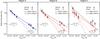 |
Fig. 4 Modeling the relative population levels of the H2 transitions using single excitation-temperature LTE models (see Davies et al. 2003). The relative population levels have been derived from the intensities of the H2 transitions listed in Table A.1. The circles and squares represent the narrow and broad component, respectively. The solid lines show the single-temperature fits using both the ν = 1 and ν = 2 transitions (i.e., assuming fully thermalized LTE gas conditions). The dashed lines show the single-temperature fits to only the ν = 1 transitions (i.e., taking into consideration that the ν = 2 transitions could be over-populated compared to fully thermalized LTE conditions). The best-fit temperatures for the narrow (n) and broad (b) component in the various regions are also show (with in brackets the temperature derive from the fit to only the ν = 1 transitions). |
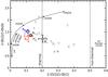 |
Fig. 5 H2 line ratio diagram for the blueshifted broad component in region A (blue square), the redshifted broad component in region B (red square) and the narrow components in regions A and B (black circles). The solid black line shows the expected line ratios for uniform density gas that is in local thermal equilibrium (LTE), with excitation temperatures indicated. The dotted lines provide an indication for the regions where the 2−1 S(1)/1−0 S(1) line ratio is caused by thermal (≲0.2) and non-thermal (≳0.5) conditions, based values from models that are summarized in Mouri (1994). The regions where these models predict UV photons (Sternberg & Dalgarno 1989), shocks/X-rays (Brand et al. 1989; Lepp & McCray 1983; Draine & Woods 1990; Dors et al. 2012) and UV-fluorescence (Black & van Dishoeck 1987) to dominate the gas excitation are indicated in more detail. Open gray symbols represent values from individual regions studied within other nearby galaxies (starforming regions, rings, arcs, clouds, etc.), with closed gray symbols the nuclei of these systems. Diamonds are from Mazzalay et al. (2013), downward pointing triangles from Falcón-Barroso et al. (2014), upwards pointing triangles from Bedregal et al. (2009) and circles from Piqueras López et al. (2012b). See also Ramos Almeida et al. (2009) and Riffel et al. (2013) for studies performed on integrated near-IR long-slit spectra of various types of galaxies. |
Apart from the H2 1−0 S(1) 2.12 μm line, we see a broad component also in other H2 lines, namely H2 1−0 S(0) 2.22 μm, 1−0 S(2) 2.03 μm, 1−0 S(3) 1.96 μm, 2−1 S(1) 2.25 μm, 2−1 S(2) 2.15 μm and 2−1 S(3) 2.07 μm. For all H2 transitions we performed a kinematic analysis similar to that of the 1−0 S(1) line. Details of this procedure, as well as the line profiles and resulting line fluxes, are provided in Appendix A.
3.1.1. Temperature and excitation mechanism
The relative intensities of the various H2 transitions can be used to discriminate between the various mechanisms that excite the H2 gas, and to estimate the gas temperature. Models show that H2 can be excited either through thermal processes, such as shocks or UV/X-ray radiation, or non-thermal processes like UV-fluorescence (e.g., Lepp & McCray 1983; Hollenbach & McKee 1989; Sternberg & Dalgarno 1989; Brand et al. 1989; Draine & Woods 1990; Maloney et al. 1996; Dors et al. 2012; Black & van Dishoeck 1987). In case of thermal processes, the H2 levels are excited through inelastic collisions, resulting in gas that is approximately in local thermal equilibrium (LTE). For gas in LTE the various H2 line ratios can be fitted by a single excitation-temperature model (see, e.g., Davies et al. 2003). In the case of non-thermal excitation, absorption of UV photons with λ> 912 Å is followed by a fluorescent cascade of electrons through the vibrational and rotational levels of the ground state. In this case, even though in most environments the lowest vibrational levels of H2 (ν = 1) are still well thermalized, the higher level transitions are significantly stronger than expected based on single-temperature LTE models and more complex models are required to derive the gas temperature (Davies et al. 2003).
To estimate the excitation temperature of the H2-emitting gas, we fit LTE models to the relative population levels across the range of H2 transitions for the various components (see Appendix A). As can be seen in Fig. 4, if a single-temperature model is fitted to both the ν = 1 and ν = 2 transitions, we derive an estimated temperature of T ~ 2000 − 2200 K. A fit to only the ν = 1 transitions renders a temperature of T ~ 1600 K, in which case the ν = 2 transitions are slightly over-populated. This indicates that the excitation conditions of the broad-component H2 gas may be somewhat more complex than single-temperature LTE conditions, with non-thermal processes adding to the gas excitation, multiple gas temperature components, or a low-density, sub-thermally excited gas phase mixed with denser LTE-gas. However, our coverage of only the ν = 1 and ν = 2 transitions, of which the ν = 2 lines are relatively weak (Fig. A.1), does not allow us to constrain the model-fitting in great detail. Moreover, as we will see in Sect. 3.2, the broad-component emission is also seen in the cold molecular CO(3−2) and CO(1−0) gas with an estimated ratio that suggests that also the cold gas may be thermalized. We therefore here adopt the temperature of T ~ 1900 ± 300 K for the broad-component emission-line gas in regions A and B.
The bright emission from the narrow-component H2 disk in regions A and B shows roughly similar temperature-estimates when fitting LTE models. However, for this narrow component, the over-population of the ν = 2 transitions is more prominent than for the broad-component emission, in particular in region B. This suggests that the temperatures of the narrow-component H2 gas are more uncertain, and that the excitation conditions in parts of the large-scale disk are likely more complex, than those of the broad-component emission. However, a detailed discussion of this is beyond the scope of this paper. For both the narrow- and broad-component emission in region C the errors in the fluxes for the various transitions are too large to derive any meaningful conclusions.
We use the H2 line ratios to further investigate the excitation-mechanism that dominates the heating of the H2 gas. Following Mouri (1994, see also Tanaka et al. 1989, we plot the ratio of the ortho-transitions 2−1 S(1)/1−0 S(1) against the ratio of the para-transitions 1−0 S(2)/1−0 S(0), which allows us to estimate whether thermal or non-thermal processes dominate the gas excitation. The results shown in Fig. 5 indicate that the gas-heating of the various components in regions A and B is dominated by thermal processes2. More specifically, the 1−0 S(2)/1−0 S(0) ratio of the various components (plotted on the y-axis of Fig. 5) is consistent with models that predict that shock or X-ray processes heat the gas, rather than that the H2 is thermally excited by UV photons (the latter would result in expected gas temperatures T ≲ 1000 K; see Mouri 1994 and references therein). The 2−1 S(1)/1−0 S(1) ratios for both the narrow and broad component in regions A and B are clearly inconsistent with what is expected when non-thermal UV-fluorescence dominates the excitation process. Within the errors, the broad-component in both region A and B falls close to the temperature of T ~ 2000 K along the LTE-line expected from uniform density gas that is fully thermalized. However, the deviation from this LTE-line indicates also here that the gas excitation may be more complex than simple LTE conditions. This is most prominent for the narrow component gas in region B, which suggests that either a non-negligible fraction of H2 excitation through non-thermal processes or a mixing of molecular gas-components with different densities may occur for the H2 gas in the large-scale disk. These results are consistent with the more detailed level population analysis of Fig. 4 that we discussed above.
3.1.2. Mass of the hot molecular gas
In Sect. 3.1.1 we showed that the H2 level populations of the broad-component emission in regions A and B are broadly consistent with hot molecular gas at a temperature of T ~ 1900 ± 300 K. This allows us to estimate the mass of the hot molecular gas following Scoville et al. (1982) and Mazzalay et al. (2013): 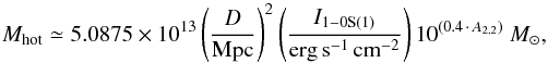 (1)where D is the distance to the galaxy and A2.2 μm the extinction at 2.2 μm. This approach assumes thermalized gas conditions and T = 2000 K, with a population fraction in the (ν,J) = (1,3) level of f(1,3) = 0.0122. As discussed in Sect. 3.1.1, the assumption of LTE conditions for the broad-component H2 gas is roughly consistent to within the accuracy of our level-population analysis, although uncertainties in this remain (for example, if a fraction of the H2 gas would be sub-thermally excited, f1,3 would be lower and Eq. (1) would thus give lower limits to the H2 mass).
According to Piqueras López et al. (2013)A2.2 μm ≈ 0.1 × AV, with AV the visual extinction. Because the broad-component H2 emission is found outside the heavily obscured nuclei, we calculate AV from the Brγ/Brδ ratio in our spectra in regions A, B and C, following Piqueras López et al. (2013). For region B we derive AV = 4.3 ± 1.3 mag, which is close to the median AV = 5 in NGC 3256 found by Piqueras López et al. (2013). For region A the Brγ and Brδ lines are too weak to derive reliable estimates, while for region C we derive AV = 0.5 ± 0.5 mag. If we assume AV = 4.3 in both region A and B, then A2.2 μm ≈ 0.1 × AV ~ 0.43. Applying this A2.2 μm results in a mass estimate of the hot molecular gas of Mhot − H2 ~ 630 and 570 M⊙ for the broad-component emission in region A and B, respectively. We note that when taking the strict lower limit of AV = 0 in region A, the corresponding mass estimate would lower by only ~33%.
Concluding, we estimate that the combined mass of hot molecular gas associated with the broad-component emission in regions A and B is Mhot − H2 ~ 1200 M⊙.
 |
Fig. 6 Total intensity map of the blueshifted (left) and redshifted (middle) high-velocity CO(3−2) emission in ALMA observations of NGC 3256. The velocity range of the integrated CO(3−2) emission is given in the plots. Overlaid are thick black contours of the broad-component H2 flux from Fig. 1 (levels from 14% to 80% in steps of 13% of the peak flux), as well as thin gray contours of the 343 GHz radio continuum from the ALMA data (levels at 3 and 10 mJy beam-1; for details see Sakamoto et al. 2014). The relative astrometry between the SINFONI and ALMA data has an estimated uncertainty of ~ 0.5′′. Right: position-velocity (PV) diagram of the high-velocity CO(3−2) emission along a north-south direction crossing the secondary nucleus at offset = 0″ (optical velocity definition; contours 20, 40, 60, 80, 100 mJy beam-1). Overlaid are black symbols that represent the broad-component H2 emission along the same direction (i.e., the NS-aperture from Fig. 1); the box shows the range between the average and maximum value per resolution element (1.1′′ × 0.25′′), while the error bars indicate ± 0.5 × FWHMaverage. The complex region of the main CO disk is not discussed (see Sakamoto et al. 2014). |
3.2. Cold molecular counterpart
In Fig. 6 we compare our broad-component H2 emission with high-velocity CO(3−2) gas (i.e., gas with velocities above those of the main CO disk), as observed with ALMA by Sakamoto et al. (2014). Figure 6 illustrates that the broad-component H2 emission of hot molecular gas in regions A and B has a counterpart in the cold molecular gas as traced by CO(3−2). The H2 and CO show a similar morphology and kinematics, which are distinctly different from that of the main CO disk (which has its kinematic axis in east-west direction at position angle ~75° and inclination ~30°; see Sakamoto et al. 2014 and Sect. 4.1). There could be a slight off-set between the location of the peak intensity for the H2 and CO(3−2) emission in regions A and B, but this is within the uncertainty of our relative astrometry. No CO counterpart of the broad-component H2 feature in region C was reliably distinguished from the main CO disk, although this is possibly due to the relatively small Δvpeak and σmax that the broad-component molecular gas will have in this region (Table 1).
We measure CO intensities of ICO(3 − 2) = 23.5 and 39.7 Jy km s-1 in region A and B (Fig. 6). From this, we can derive mass estimates of the cold molecular gas if we know the excitation conditions of the gas. The high-velocity gas was also detected in CO(1−0) by Sakamoto et al. (2014) at lower spatial resolution. Through a basic comparison of the high-velocity component in the CO(3−2) and CO(1−0) data, we estimate that  /
/ is close to unity for regions A and B, and thus broadly consistent with thermal excitation conditions. This takes into account that for region B Sakamoto et al. (2014) estimate that ~34% of the high-velocity CO(3−2) emission and ~72% of the CO(1−0) emission is contaminated by a CO outflow originating from the primary nucleus. If we assume /
 and we exclude the ~34% contamination of high-velocity CO(3−2) emission from the primary nucleus in region B, we can set a lower-limit estimate to the luminosity of the cold molecular gas of
  K km s-1 pc2 for region A and
  K km s-1 pc2 for region B (see Solomon & Vanden Bout 2005). By adopting a standard conversion factor for ULIRGs of
  (Downes & Solomon 1998), this translates into a conservative estimate of the cold molecular gas of Mcold − H2 ≈ 1.0 and 1.1 × 10⁷M⊙ for region A and B respectively, or Mcold − H2 ≈ 2.1 × 10⁷M⊙ in total. Sakamoto et al. (2014) use the CO(1−0) intensity to estimate a total mass of 4.1 × 107X20M⊙ for this high-velocity gas (assuming
  and adjusted for our assumed D = 44.6 Mpc to NGC 3256). Our assumption of αCO = 0.8 translates to X20 ~ 0.4 (see Bolatto et al. 2013). Therefore, taking into consideration the uncertainties involved regarding contamination of outflowing gas from the primary nucleus, our adopted αCO = 0.8, and the gas thermalization, the two approaches agree to a mass of at least Mcold − H2 ~ 2 × 10⁷M⊙ of cold molecular gas associated with the broad-component H2 feature in regions A and B. We will use this value throughout the rest of this paper.
For further details on the CO data we refer to Sakamoto et al. (2014).
4. Discussion
We presented broad-component H2 emission-line features of hot molecular hydrogen gas in the vicinity of the heavily obscured secondary nucleus of NGC 3256. We here discuss the nature of the broad-component H2 emission in regions A and B. We present three possible scenarios: a biconical molecular gas outflow, a rotating disk that revolves around the secondary nucleus and a pair of tidal features. We will show that a molecular gas outflow best explains the observed properties (Sect. 4.1). The fact that this outflow is detected at high spatial resolution in both the hot and cold molecular gas phase makes it one of the few molecular outflows for which we can study in detail the physical structure and properties (Sect. 4.2). We will also investigate the driving mechanism of the outflow (Sect. 4.3) and conclude with a brief remark about how our results fit into the broader perspective on molecular gas outflows (Sect. 4.4).
4.1. Nature of the broad-component H2 emission
The first scenario to explain the broad-component H2 emission in regions A and B is that of a kpc-scale biconical outflow of molecular gas that originates from the secondary nucleus. We will here show that this scenario explains well the geometry and kinematics of the observed H2 features. In Fig. 7 we visualize the geometry of the large-scale molecular gas disk and the biconical outflow from the secondary nucleus, as suggested by Sakamoto et al. (2014). The ALMA CO data of Sakamoto et al. (2014) reveal that the large-scale disk has an inclination of ~30° and that the southern part of the large-scale disk is the near side if the tidal-tails are trailing. They also show that the orbital plane of the primary and secondary nucleus must be close to this large-scale gas disk, but that the secondary is in front of the primary core and the secondary’s nuclear disk has an inclination of at least idisk ~ 70°. If we assume that the outflow is perpendicular to the nuclear disk, this would render the molecular outflow close to the plane of the sky (ioutfl ~ 20°). A biconical molecular gas outflow in a system with this geometry would explain why we see blueshifted H2 emission in region A and redshifted emission in region B. In addition, the geometry in Fig. 7 suggests that the outflow may interact with the large-scale disk in region A. If this interaction results in shock-heating of molecular gas, this can naturally explain the fact that in region A the enhanced flux of H2 emission in the outflowing broad-component gas is co-spatial with an enhancement in the H2 flux of the narrow-component gas disk (Fig. 1). Concluding, the observed geometry and kinematics of the broad-component H2 emission agree with what is expected from a molecular outflow.
 |
Fig. 7 Alignment between the (nuclear) disks of the progenitor galaxies associated with the primary/secondary nucleus and the H2 outflow. The alignment of the nuclear disks is based on CO observations by Sakamoto et al. (2014). Simplistically, the large-scale disks and tidal tails of the progenitor galaxies are assumed to be aligned parallel to the nuclear disks. |
A second scenario is that the broad-component H2 emission is an edge-on molecular disk or ring that rotates around the secondary nucleus. The velocity dispersion of the broad-component H2 emission in NGC 3256 is distinctively larger than that of the main gas disk (Sect. 3.1), with v/σ ~ 1.3. This is intermediate between that of rotation-dominated (v/σ ≳ 1) and random-motion-dominated (v/σ ≲ 1) systems (e.g., Epinat et al. 2012; Bellocchi et al. 2013), suggesting resemblance to a “thick disk”, rather than a classical “thin disk”. However, two arguments make this scenario unlikely. First, the dynamical mass enclosed by this rotating structure would be  , although following Bellocchi et al. (2013) it could be as high as
  if we take into account the velocity dispersion of the gas (assuming vrot = Δvpeak = 250 km s-1, σ = 190 km s-1, R = 700 pc and G = 6.67 × 10⁻¹¹ m3 kg-1 s-2 the gravitational constant; Table 1). This would result in a gas mass to dynamical mass ratio of Mgas/Mdyn ≈ 1/500 − 1/1500. This is two orders of magnitude below the typical value of Mgas/Mdyn ≈ 1/6 observed for the main central molecular gas disks of ULIRGs (Downes & Solomon 1998). Second, a rotating disk or ring would cross the large-scale primary disk, which would trigger cloud-cloud collisions that would make the structure very unstable and short-lived. We thus argue that a rotating disk or ring is not a likely alternative explanation for the broad-component H2 emission in regions A and B.
A third scenario is that the broad-component H2 emission in regions A and B represents tidal features that are not in dynamical equilibrium. The complex kinematics observed within NGC 3256 make this an attractive alternative scenario to investigate. The interaction between the putative tails and the ISM in regions A and B could increase the velocity dispersion of the gas within the tails. However, the observed broad-component features in regions A and B are only detected in the molecular gas phase and have no clear stellar or dusty counterparts, as would be expected for tidal tails (Fig. 3). In addition, the spatial and kinematic geometry of the broad-component structure with respect to the secondary nucleus strongly suggests that the tidal gas would have been stripped off the secondary’s central disk. However, Sakamoto et al. (2014) show that the merger orbital plane is close to face-on and they therefore argue that the tidal force between the primary and secondary nucleus cannot produce large line-of-sight velocities for gas that is stripped off the secondary’s central disk. Thus, the currently available data do not seem to favor the scenario that the broad-component H2 emission reflects tidal features.
4.2. Detailed physical properties of the outflow
In Sect. 4.1 we argued that a biconical molecular gas outflow best explains the observed properties of the broad-component H2 emission in regions A and B. The high spatial resolution of our data reveals interesting physical properties of the outflow. From the narrow width of the H2 outflow in EW-direction (≲300 pc), our data indicate that the outflow has an opening angle of ~40°. The highest-velocity H2 gas is found 440 (800) pc south (north) of the secondary nucleus. This suggests that the molecular outflow peaks far from the nucleus, possibly resembling a biconical shell-like geometry, with the lower-velocity molecular gas found down-stream of this shell.
The hot-to-cold molecular gas mass ratio of the outflowing gas is ~6 × 10⁻⁵, which is at the high end of the range 10-7–10-5 observed across a sample of several dozen star-forming galaxies and AGN by Dale et al. (2005). Moreover, H2 has a short cooling timescale of ~104 yr, which is two orders of magnitude shorter than the gas outflow timescale that we will calculate below (toutfl ~ 106 yr). This suggests that molecular gas in the outflow may be continuously shocked or heated (as is also observed to be the case for a molecular outflow from the radio-loud ULIRG PKS 1345+12; Dasyra et al. 2014.) The fact that the outflow appears to be predominantly molecular (Sect. 3.1) suggests that the gas is most likely entrained in a wind from the AGN/starburst region, possibly by dragging molecular gas out of the secondary’s circum-nuclear disk. This gas is likely heated through relatively slow shocks or X-rays (potentially from the AGN) to our observed temperature of ~1900 K. It is not immediately apparent that the H2 emission could represent a transient phase of gas-cooling after fast shocks accelerate and heat/ionize gas directly at the shock-front (as appears to happen in the nearby active galaxy IC 5063; Tadhunter et al. 2014), because we do not see evidence of copious amounts of ionized gas in Brγ that one would expect to be created by such fast shocks.
In Sect. 3.1 we found that the kinematic signature of the outflowing H2 gas has an observed FWZI ≈ 1200 km s-1, which means that the molecular gas in the outflow reaches a maximum line-of-sight velocity of ±600 km s-1. If we follow the outflow geometry described in Sect. 4.1 and Fig. 7, with ioutfl ~ 20°, this means that the intrinsic outflow velocities can reach a maximum of about ±1800 km s-1. Similarly, if we assume our observed average outflow velocity to be vavg = 0.5 × FWHMtot ≈ 280 km s-1, this translates into an intrinsic average velocity of vavg ~ 280 sin-1(ioutfl) ~ 820 km s-1. If we also de-project the outflow radius to R = 700 cos-1(ioutfl) ~ 750 pc, this means that it would take the gas roughly 106 yr to travel this distance. We note that Sakamoto et al. (2014) argue that the inclination of the outflow axis could even be as low as ioutfl ~ 5°, which would increase the above mentioned intrinsic outflow velocities with a factor of ~4. Sakamoto et al. (2014) base this low value for ioutfl on the fact that blue- and redshifted CO emission are observed to be co-spatial within the conical outflow, which they argue means that the inclination of the outflow is less than half the opening angle of ~20° that they measure from their CO data (i.e., ioutflow ≤ 10°). However, this does not take into account the large velocity dispersion that we measure for the H2 gas, which could explain the co-spatial red- and blueshifted emission even when ioutfl> 10°. In addition, we find an opening angle for the outflow of ~40°, larger than the ~20° that Sakamoto et al. (2014) derived from the CO data. We therefore argue that ioutfl< 20° is not required to explain the observed properties of the molecular outflow.
With an intrinsic vavg ~ 820 km s-1, R ~ 750 pc and a total molecular gas mass of ~2 × 10⁷M⊙ involved in the outflow, the average mass outflow rate is Ṁoutfl ~ 20 M⊙ yr-1. This is similar to that of other molecular outflows observed in low-z starburst galaxies and AGN (e.g., Alatalo et al. 2011; Morganti et al. 2013b; Cicone et al. 2014; Garcia-Burillo et al. 2014, see also Sect. 1). This value for Ṁoutfl is likely a lower limit, because our estimate of Ṁoutfl is based on the over-simplified assumption that the total gas mass is driven out in a single event. As we discussed above, it is possible that the outflow is shell-like, or at least continuously re-filled with outflowing clouds, in which case Ṁout can be larger by at least a factor of a few (see Maiolino et al. 2012; Cicone et al. 2014). Still, Ṁoutfl ~ 20 M⊙ yr-1 is high compared to the star-formation rate of the secondary nucleus. Following to Kotilainen et al. (1996) and Piqueras López (2014), the star-formation rate in the secondary nucleus is SFR ~1−3 M⊙ yr-1 (corrected for estimated extinctions of AV ~ 10−12 mag). Although significant uncertainty remains in these estimates, the mass-loading factor could be as high as η = Ṁout/SFR ~ 10.
4.3. Outflow mechanism: AGN vs. starburst
The relatively high mass loading factor of the outflow (η = Ṁout/SFR ~ 10) indicates that there is a discrepancy between the mass outflow rate and star-formation rate. A similar result on a molecular outflow in the nearby Seyfert galaxy NGC 1068 led Garcia-Burillo et al. (2014) to favor AGN activity over star formation as the likely mechanism to drive the outflow (based on work by Murray et al. 2005 and Veilleux et al. 2005). Moreover, the morphology of the H2 outflow from the secondary nucleus in NGC 3256 reveals that the outflow is rather collimated with an opening angle of ~40°, while the instrinsic maximum outflow velocity is high (vmax ~ 1800 km s-1). Arribas et al. (2014) show that AGN in (U)LIRGs generate ionized gas outflows that are twice as fast as those produced by starbursts in these systems. These results could suggest that a hidden AGN may contribute to driving the outflow, for example through radiation pressure or a magnetically driven accretion-disk wind (e.g., Everett 2005; Proga 2007). Sakamoto et al. (2014) also show marginal evidence for the presence of a faint two-sided radio-jet emanating from the secondary nucleus, which appears to be aligned with the high-velocity CO(3−2) emission (based on data from Neff et al. 2003). Still, unambiguous observational evidence for the presence of an AGN in the secondary nucleus is currently lacking (Sect. 1). So are at least the energetics of the outflow consistent with the scenario that a hidden AGN, or else the nuclear starburst, can drive the outflow?
The combined turbulent and bulk kinetic energy of the molecular outflow, ![Mathematical equation: \begin{equation} E_{\rm tot} = E^{\rm turb}_{\rm kin} + E^{\rm bulk}_{\rm kin} = {\frac{3}{2}} \cdot {M}\sigma^{2} + {\frac{1}{2}} \cdot {M}{[v/\sin({\it i}_{\rm outfl})]}^{2}, \end{equation}](/articles/aa/full_html/2014/12/aa23805-14/aa23805-14-eq159.png) (2)is Etot ~ 2 × 1056 erg (for M ≈ 2 × 10⁷M⊙, σ ≈ 190 km s-1, v ≈ 280 km s-1 and ioutfl = 20°). We first compare this to the radiation from a potential AGN accretion disk. The 0.5−10 keV X-ray luminosity from the secondary nucleus is LX ~ 3 × 1040 erg s-1 (assuming a power-law spectral model with Γ = 2.0 and an absorbing column of 5 × 1022 cm-2; Lira et al. 2002). Elvis et al. (1994) show that QSOs with L1 − 10 keV ~ 1043 − 47 erg s-1 have a bolometric luminosity Lbol that is 5−50 × larger than L1 − 10 keV, with an average/median value of Lbol/L1 − 10 keV ~ 20. Ho (2008) estimate a similar value of Lbol/L2 − 10 keV ~ 16 for low-luminosity AGN. Lira et al. (2002) show that most of the 0.5−10 keV X-ray emission from the secondary nucleus of NGC 3256 occurs in the hard 2−10 keV regime, so if we simplistically assume that the X-ray emission comes from a hidden AGN and we apply Lbol/LX ~ 16, then the bolometric AGN luminosity would be Lbol ~ 5 × 1041 erg s-1 in case the AGN would be X-ray – transparent or Compton-thin. Over the outflow timescale of 106 yr, the total energy deposited by the AGN would be ~2 × 1055 erg s-1, an order of magnitude too low to drive the outflow. However, if the X-ray emission is scattered emission from a Compton-thick (i.e., X-ray-obscured) AGN, the AGN’s intrinsic LX, and thus also Lbol, can be be a factor of 60−70 higher (Panessa et al. 2006; Singh et al. 2011). The non-detection of the Fe α line at 6.4 keV has led Pereira-Santaella et al. (2011) to conclude that the upper limit to Lbol for a Compton-thick AGN is on the order of 1043 erg s-1 in NGC 3256. Still, when adopting this upper limit, it would imply that a Compton-thick AGN, in case it has remained active over the past ~106 yr, may have released a total energy of up to ~3 × 1056 erg s-1 over this period, which would have been sufficient to drive the outflow.
(2)is Etot ~ 2 × 1056 erg (for M ≈ 2 × 10⁷M⊙, σ ≈ 190 km s-1, v ≈ 280 km s-1 and ioutfl = 20°). We first compare this to the radiation from a potential AGN accretion disk. The 0.5−10 keV X-ray luminosity from the secondary nucleus is LX ~ 3 × 1040 erg s-1 (assuming a power-law spectral model with Γ = 2.0 and an absorbing column of 5 × 1022 cm-2; Lira et al. 2002). Elvis et al. (1994) show that QSOs with L1 − 10 keV ~ 1043 − 47 erg s-1 have a bolometric luminosity Lbol that is 5−50 × larger than L1 − 10 keV, with an average/median value of Lbol/L1 − 10 keV ~ 20. Ho (2008) estimate a similar value of Lbol/L2 − 10 keV ~ 16 for low-luminosity AGN. Lira et al. (2002) show that most of the 0.5−10 keV X-ray emission from the secondary nucleus of NGC 3256 occurs in the hard 2−10 keV regime, so if we simplistically assume that the X-ray emission comes from a hidden AGN and we apply Lbol/LX ~ 16, then the bolometric AGN luminosity would be Lbol ~ 5 × 1041 erg s-1 in case the AGN would be X-ray – transparent or Compton-thin. Over the outflow timescale of 106 yr, the total energy deposited by the AGN would be ~2 × 1055 erg s-1, an order of magnitude too low to drive the outflow. However, if the X-ray emission is scattered emission from a Compton-thick (i.e., X-ray-obscured) AGN, the AGN’s intrinsic LX, and thus also Lbol, can be be a factor of 60−70 higher (Panessa et al. 2006; Singh et al. 2011). The non-detection of the Fe α line at 6.4 keV has led Pereira-Santaella et al. (2011) to conclude that the upper limit to Lbol for a Compton-thick AGN is on the order of 1043 erg s-1 in NGC 3256. Still, when adopting this upper limit, it would imply that a Compton-thick AGN, in case it has remained active over the past ~106 yr, may have released a total energy of up to ~3 × 1056 erg s-1 over this period, which would have been sufficient to drive the outflow.
How about mechanical energy from the putative radio source? As shown by Sakamoto et al. (2014, their Fig. 19), the weak radio source appears to have a two-sided jet with a total 8 GHz radio flux of at most F8 GHz ~ 1 mJy (i.e., not taking into account the nuclear emission). From the flux of the jet we can derive the bulk kinetic power of the radio source by following Willott et al. (1999) and Godfrey & Shabala (2013): 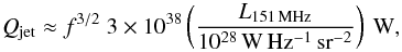 (3)where L151 MHz is the 151 MHz luminosity (derived from the 151 MHz flux and luminosity distance through
  ) and f is a factor that represents errors in the model assumption, including the excess energy in particles compared with that in the magnetic field, geometrical effects and energy in the backflow of the lobe (see Willott et al. 1999 and Blundell & Rawlings 2000 for details). Following Blundell & Rawlings (2000), the value of f is typically around 10−20, so here we assume f = 15. In the optimistic case that the jet has a steep radio spectrum with Sν ∝ ν-1, thus F151 ~ 55 mJy, we estimate that Qjet ~ 2 × 1040 erg s-1. Over a typical radio-source lifetime of 106 yr, the mechanical energy deposited by the radio source would only be on the order of ~6 × 1053 erg. This is two orders of magnitude lower than the combined turbulent and bulk kinetic energy of the molecular outflow, which suggests that the putative radio source currently does not have the power that is required to drive the outflow. Still, the presence of a radio source carving its way through the ISM may potentially have aided in creating a cavity through which molecular gas can be efficiently accelerated.
Alternatively, can the necessary energy for driving the outflow be injected by a nuclear starburst? Kotilainen et al. (1996) and Norris & Forbes (1995) derive a supernova-rate in the secondary nucleus of RSN ~ 0.3 SN yr-1. Assuming an energy-release per supernova event of ~1051 erg (Bethe & Pizzochero 1990), and the fact that up to 90% of the energy per supernova is likely radiated away (Thornton et al. 1998), the total energy deposited into the ISM by supernovae over the course of the outflow timescale toutfl is roughly  (4)with ϵ the assumed efficiency of energy transfer to the ISM. For RSN ~ 0.3 SN yr-1, ϵ ~ 0.1 and toutfl ~ 106 yr, the energy-deposition by supernovae is ESN = 3 × 1055 ergs. Stellar winds will release additional energy into the system, although Leitherer et al. (1992) show that once the starburst has aged enough that supernova-explosions occur, stellar winds will increase the total energy deposited into the ISM by at most a factor of 2, putting a limit of ESN + winds ~ 6 × 1055 erg. This is only a factor of 3 lower than the energy of the outflow. Given the assumptions involved, and the fact that it is uncertain to what extent the large amounts of radiative energy may contribute to driving the outflow, it is possible that the energy output of the starburst event in the secondary nucleus may be sufficient to sustain the outflow.
Concluding, the high mass loading factor, high outflow velocities and substantial collimation of the outflow suggest that that a hidden AGN may contribute to driving the outflow of molecular gas from the secondary nucleus. Based on the energetics, we argue that the most plausible way a hidden AGN can drive the outflow is in the Compton-thick regime, through radiation-pressure or an accretion-disk wind. However, the scenario that the nuclear starburst provides the energy needed to drive the outflow is also possible.
4.4. Broader perspective
Interestingly, while the biconical structure of the outflow shows a distinct blue- and redshifted wing to the emission-line profile on either side of the secondary nucleus, when integrated across the entire outflow region the broad-component profile appears symmetric with respect to the assumed systemic velocity of the secondary nucleus (Fig. 2). This is similar to what is often seen in CO data with much lower spatial resolution, and for objects at intermediate- and high-z (e.g., Feruglio et al. 2010; Maiolino et al. 2012; Cicone et al. 2014). Thus, our results provide valuable insight into understanding the structural properties of starburst/AGN-driven molecular gas outflows in general.
5. Conclusions
We presented evidence for the presence of a kpc-scale biconical outflow of hot molecular gas from the heavily obscured secondary nucleus of NGC 3256, based on near-IR 2.12 μm H2 data obtained with VLT/SINFONI. Our main conclusions are:
-
i)
The outflow is observed at high spatial resolution in both the hot molecular gas phase with VLT/SINFONI (H2) and the cold molecular phase with ALMA (CO). The hot and cold component of the molecular outflow share a similar morphology and kinematics.
-
ii)
These data allowed us to characterize the geometry, kinematics and physical properties of the molecular outflow. In particular:
-
The outflow consists of a blueshifted outflow-component south and a redshifted component north of the secondary nucleus, with an opening angle of ~ 40°;
-
The emission-line kinematics show observed maximum outflow velocities of ±600 km s-1. However, give the low inclination of the jet-axis (ioutfl ~ 20°), intrinsic outflow velocities can reach a maximum of ~1800 km s-1;
-
The mass of the hot molecular gas in the outflow is Mhot H2 ~ 1200 M⊙, while the outflowing cold molecular gas mass is Mcold H2 ~ 2 × 10⁷M⊙. This results in a hot-to-cold molecular gas mass ratio of ~ 6 × 10⁻⁵ and total molecular mass-outflow rate of at least Ṁoutfl ~ 20 M⊙ yr-1;
-
From the analysis of multiple near-IR H2-transitions, we derive a temperature of T ~ 1900 ± 300 K for the hot H2 gas in the outflow. The likely heating mechanism is either shocks or X-ray emission.
-
-
iii)
A likely driving mechanism for the molecular outflow is ahidden AGN, given the high mass-loading factor(η ~ 10), high outflow velocities and significant collimation of the outflowing gas. Based on energy requirements, this would most likely happen in the Compton-thick regime, through radiation pressure or an accretion-disk wind. Alternatively, the nuclear starburst may potentially provide enough energy to drive the outflow;
-
iv)
When integrated over the outflow region, the global kinematics of the outflowing molecular gas mimic those observed with low-resolution CO observations in other low- and high-z objects. The structural and physical properties of the molecular outflow in NGC 3256 that we derive from our high-resolution data therefore provide valuable insight into our general understanding of starburst/AGN-driven molecular gas outflows.
Online material
Appendix A: Properties H2 transitions
In this Appendix we provide the spectra and line fluxes derived from fitting two Gaussian components to the emission-line spectra of the various H2 transitions in regions A, B and C.
Appendix A.1: Method
For each of the seven H2 transitions in our SINFONI data we extracted an emission-line spectrum from a circular aperture of 13 spaxels centered around the peak flux in regions A, B and C (similar to what is shown in Fig. 1 for H2 1−0 S(1)).
As mentioned in Sect. 2, we used an IDL routine based on the MPFIT package to perform the line-fitting. We used a three-component model to simultaneously fit the continuum and both the narrow and broad component of the emission lines. The continuum was fitted using a linear term, whereas a Gaussian profile was used for each emission-line component.
As can be seen in Fig. A.1, the signal-to-noise of some of the lines is too low to derive accurate results when using this multi-component analysis without placing any constraints on the line-fitting procedure. To reduce the uncertainties of the fitting and obtain more robust measurements of the line fluxes, we assume that all transitions share the same kinematics. We first performed
the fitting routine on the strong 1−0 S(1) 2.1218 μm line without placing constraints on the line-fitting parameters. Subsequently, we used these results to fix the position and line width (both in km s-1) of the narrow and broad component of the other emission lines.
The uncertainties of the flux measurements were calculated using a Monte Carlo technique. This method consists of measuring the noise in the spectra as the root-mean-square of the residuals after the subtraction of our multi-component model. Taking this estimation of the noise into account, we construct a total of 500 independent simulations/realizations of the spectra, where the lines are again fitted. These simulations yield distributions of each free parameter of our model. The uncertainty of each parameter is then defined as the standard deviation of its corresponding distribution.
Appendix A.2: Results
In Fig. A.1 we show the results of the line-fitting procedure. In Table A.1 we summarize the line ratios for the broad and narrow component with respect to the flux of the 1−0 S(1) 2.1218 μm line. The upper limits are defined as 1-sigma detections, using the noise estimation from the Monte Carlo method described in Sect. A.1.
Flux ratios of the broad and narrow components of all seven H2 lines in our SINFONI data with respect to 1−0 S(1) in regions A, B and C.
 |
Fig. A.1 Emission-line spectra and 2-component Gaussian fit of the various H2 transitions in regions A, B and C. The spectra were extracted from a circular aperture of 13 spaxels, centered on the broad-component H2 feature in each region. The line width and shift between the peak of the narrow and broad component were constrained in velocity to those of the strong 1−0 S(1) line. A straight line was fitted to the continuum across a wide velocity range of −1800 to +1800 km s-1 in order to handle potential features in the continuum (see, e.g., the H2 1−0S(3) transition in region B). However, a smaller velocity range is plotted in the figures to high-light the details of the fits to the emission lines. After extracting flux measurements, for visualisation purposes the spectra in the plots were normalized to the fitted continuum. |
Because of residual sky-line effects at the very edge of the SINOFONI wavelength coverage, we could not do an accurate spectral analysis of the H2 1−0Q(1) and H2 1−0Q(2) lines.
Acknowledgments
We thank the anonymous referee for valuable suggestions that substantially improved the content of this paper. BE is grateful that the research leading to these results has received funding from the Spanish Ministerio de Economía y Competitividad (MINECO) under grant AYA2010-21161-C02-01 and from the European Union Seventh Framework Programme (FP7-PEOPLE-2013-IEF) under grant agreement n° 624351. L.C., S.A. and A.A.H. acknowledge support through MINECO grants AYA-2012-39408-C02-01 and AYA-2012-31447. M.P.S. is supported by the Agenzia Spaziale Italiana (ASI), contract I/005/11/0. Based on observations collected at the European Organisation for Astronomical Research in the Southern Hemisphere, Chile, prog. 078.B-0066A. This paper makes use of the following ALMA data: ADS/JAO.ALMA#2011.0.00525.S. ALMA is a partnership of ESO (representing its member states), NSF (USA) and NINS (Japan), together with NRC (Canada) and NSC and ASIAA (Taiwan), in cooperation with the Republic of Chile. The Joint ALMA Observatory is operated by ESO, AUI/NRAO and NAOJ. Based on observations made with the NASA/ESA Hubble Space Telescope, and obtained from the Hubble Legacy Archive, which is a collaboration between the Space Telescope Science Institute (STScI/NASA), the Space Telescope European Coordinating Facility (ST-ECF/ESA) and the Canadian Astronomy Data Centre (CADC/NRC/CSA).
References
- Aalto, S., Booth, R. S., Johansson, L. E. B., & Black, J. H. 1991, A&A, 247, 291 [Google Scholar]
- Aalto, S., Muller, S., Sakamoto, K., et al. 2012, A&A, 546, A68 [NASA ADS] [CrossRef] [EDP Sciences] [Google Scholar]
- Alatalo, K., Blitz, L., Young, L. M., et al. 2011, ApJ, 735, 88 [NASA ADS] [CrossRef] [Google Scholar]
- Alonso-Herrero, A., Colina, L., Packham, C., et al. 2006a, ApJ, 652, L83 [NASA ADS] [CrossRef] [Google Scholar]
- Alonso-Herrero, A., Rieke, G. H., Rieke, M. J., et al. 2006b, ApJ, 650, 835 [NASA ADS] [CrossRef] [Google Scholar]
- Alonso-Herrero, A., Pereira-Santaella, M., Rieke, G. H., & Rigopoulou, D. 2012, ApJ, 744, 2 [NASA ADS] [CrossRef] [Google Scholar]
- Arribas, S., Colina, L., Bellocchi, E., Maiolino, R., & Villar-Martin, M. 2014, A&A, 568, A14 [NASA ADS] [CrossRef] [EDP Sciences] [Google Scholar]
- Baan, W. A., Henkel, C., Loenen, A., et al. 2008, A&A, 477, 747 [NASA ADS] [CrossRef] [EDP Sciences] [Google Scholar]
- Bedregal, A. G., Colina, L., Alonso-Herrero, A., & Arribas, S. 2009, ApJ, 698, 1852 [NASA ADS] [CrossRef] [Google Scholar]
- Bellocchi, E., Arribas, S., Colina, L., & Miralles-Caballero, D. 2013, A&A, 557, A59 [NASA ADS] [CrossRef] [EDP Sciences] [Google Scholar]
- Bethe, H. A., & Pizzochero, P. 1990, ApJ, 350, L33 [NASA ADS] [CrossRef] [Google Scholar]
- Black, J. H., & van Dishoeck, E. F. 1987, ApJ, 322, 412 [NASA ADS] [CrossRef] [Google Scholar]
- Blundell, K. M., & Rawlings, S. 2000, AJ, 119, 1111 [NASA ADS] [CrossRef] [Google Scholar]
- Bolatto, A. D., Wolfire, M., & Leroy, A. K. 2013, ARA&A, 51, 207 [Google Scholar]
- Bonnet, H., Abuter, R., Baker, A., et al. 2004, The Messenger, 117, 17 [NASA ADS] [Google Scholar]
- Brand, P. W. J. L., Toner, M. P., Geballe, T. R., et al. 1989, MNRAS, 236, 929 [NASA ADS] [CrossRef] [Google Scholar]
- Casoli, F., Dupraz, C., & Combes, F. 1992, A&A, 264, 49 [NASA ADS] [Google Scholar]
- Cazzoli, S., Arribas, S., Colina, L., et al. 2014, A&A, 569, A14 [NASA ADS] [CrossRef] [EDP Sciences] [Google Scholar]
- Chung, A., Yun, M. S., Naraynan, G., Heyer, M., & Erickson, N. R. 2011, ApJ, 732, L15 [NASA ADS] [CrossRef] [Google Scholar]
- Cicone, C., Maiolino, R., Sturm, E., et al. 2014, A&A, 562, A21 [NASA ADS] [CrossRef] [EDP Sciences] [Google Scholar]
- Combes, F., García-Burillo, S., Casasola, V., et al. 2013, A&A, 558, A124 [NASA ADS] [CrossRef] [EDP Sciences] [Google Scholar]
- Dale, D., Sheth, K., Helou, G., Regan, M., & Hüttemeister, S. 2005, AJ, 129, 2197 [NASA ADS] [CrossRef] [Google Scholar]
- Dasyra, K. M., & Combes, F. 2012, A&A, 541, L7 [NASA ADS] [CrossRef] [EDP Sciences] [Google Scholar]
- Dasyra, K. M., Combes, F., Novak, G. S., et al. 2014, A&A, 565, A46 [NASA ADS] [CrossRef] [EDP Sciences] [Google Scholar]
- Davies, R. I., Sternberg, A., Lehnert, M., & Tacconi-Garman, L. E. 2003, ApJ, 597, 907 [NASA ADS] [CrossRef] [Google Scholar]
- Díaz-Santos, T., Alonso-Herrero, A., Colina, L., et al. 2008, ApJ, 685, 211 [NASA ADS] [CrossRef] [Google Scholar]
- Dors, Jr., O. L., Riffel, R. A., Cardaci, M. V., et al. 2012, MNRAS, 422, 252 [NASA ADS] [CrossRef] [Google Scholar]
- Downes, D., & Solomon, P. M. 1998, ApJ, 507, 615 [NASA ADS] [CrossRef] [Google Scholar]
- Doyon, R., Joseph, R. D., & Wright, G. S. 1994, ApJ, 421, 101 [NASA ADS] [CrossRef] [Google Scholar]
- Draine, B. T., & Woods, D. T. 1990, ApJ, 363, 464 [NASA ADS] [CrossRef] [Google Scholar]
- Eisenhauer, F., Abuter, R., Bickert, K., et al. 2003, in SPIE Conf. Ser. 4841, eds. M. Iye, & A. F. M. Moorwood, 1548 [Google Scholar]
- Elvis, M., Wilkes, B. J., McDowell, J. C., et al. 1994, ApJS, 95, 1 [NASA ADS] [CrossRef] [Google Scholar]
- English, J., Koribalski, B., Bland-Hawthorn, J., Freeman, K. C., & McCain, C. F. 2010, AJ, 139, 102 [NASA ADS] [CrossRef] [Google Scholar]
- Epinat, B., Tasca, L., Amram, P., et al. 2012, A&A, 539, A92 [NASA ADS] [CrossRef] [EDP Sciences] [Google Scholar]
- Everett, J. E. 2005, ApJ, 631, 689 [NASA ADS] [CrossRef] [Google Scholar]
- Falcón-Barroso, J., Ramos Almeida, C., Böker, T., et al. 2014, MNRAS, 438, 329 [NASA ADS] [CrossRef] [Google Scholar]
- Feruglio, C., Maiolino, R., Piconcelli, E., et al. 2010, A&A, 518, L155 [NASA ADS] [CrossRef] [EDP Sciences] [Google Scholar]
- Garcia-Burillo, S., Combes, F., Usero, A., et al. 2014, A&A, 567, A125 [NASA ADS] [CrossRef] [EDP Sciences] [Google Scholar]
- Godfrey, L. E. H., & Shabala, S. S. 2013, ApJ, 767, 12 [NASA ADS] [CrossRef] [Google Scholar]
- Guillard, P., Ogle, P. M., Emonts, B. H. C., et al. 2012, ApJ, 747, 95 [NASA ADS] [CrossRef] [Google Scholar]
- Heckman, T. M., Armus, L., & Miley, G. K. 1990, ApJS, 74, 833 [NASA ADS] [CrossRef] [Google Scholar]
- Heckman, T. M., Lehnert, M., Strickland, D., & Armus, L. 2000, ApJS, 129, 493 [NASA ADS] [CrossRef] [MathSciNet] [Google Scholar]
- Ho, L. C. 2008, ARA&A, 46, 475 [NASA ADS] [CrossRef] [Google Scholar]
- Hollenbach, D., & McKee, C. F. 1989, ApJ, 342, 306 [NASA ADS] [CrossRef] [Google Scholar]
- Jenkins, L. P., Roberts, T. P., Ward, M. J., & Zezas, A. 2004, MNRAS, 352, 1335 [NASA ADS] [CrossRef] [Google Scholar]
- Kotilainen, J. K., Moorwood, A., Ward, M., & Forbes, D. 1996, A&A, 305, 107 [NASA ADS] [Google Scholar]
- Laine, S., van der Marel, R. P., Rossa, J., et al. 2003, AJ, 126, 2717 [NASA ADS] [CrossRef] [Google Scholar]
- Leitherer, C., Robert, C., & Drissen, L. 1992, ApJ, 401, 596 [NASA ADS] [CrossRef] [Google Scholar]
- Leitherer, C., Chandar, R., Tremonti, C. A., Wofford, A., & Schaerer, D. 2013, ApJ, 772, 120 [NASA ADS] [CrossRef] [Google Scholar]
- Leon, S., Eckart, A., Laine, S., et al. 2007, A&A, 473, 747 [NASA ADS] [CrossRef] [EDP Sciences] [Google Scholar]
- Lepp, S., & McCray, R. 1983, ApJ, 269, 560 [NASA ADS] [CrossRef] [Google Scholar]
- Lípari, S., Díaz, R., Taniguchi, Y., et al. 2000, AJ, 120, 645 [NASA ADS] [CrossRef] [Google Scholar]
- Lípari, S. L., Díaz, R. J., Forte, J. C., et al. 2004, MNRAS, 354, L1 [NASA ADS] [CrossRef] [Google Scholar]
- Lira, P., Ward, M., Zezas, A., Alonso-Herrero, A., & Ueno, S. 2002, MNRAS, 330, 259 [NASA ADS] [CrossRef] [Google Scholar]
- Lira, P., Gonzalez-Corvalan, V., Ward, M., & Hoyer, S. 2008, MNRAS, 384, 316 [NASA ADS] [CrossRef] [Google Scholar]
- Mahony, E. K., Morganti, R., Emonts, B. H. C., Oosterloo, T. A., & Tadhunter, C. 2013, MNRAS, 435, L58 [NASA ADS] [CrossRef] [Google Scholar]
- Maiolino, R., Gallerani, S., Neri, R., et al. 2012, MNRAS, 425, L66 [NASA ADS] [CrossRef] [Google Scholar]
- Maloney, P. R., Hollenbach, D. J., & Tielens, A. G. G. M. 1996, ApJ, 466, 561 [NASA ADS] [CrossRef] [Google Scholar]
- Markwardt, C. B. 2009, ASP Conf. Ser. 411, eds. D. A. Bohlender, D. Durand, & P. Dowler, 251 [Google Scholar]
- Mazzalay, X., Saglia, R. P., Erwin, P., et al. 2013, MNRAS, 428, 2389 [NASA ADS] [CrossRef] [Google Scholar]
- Mirabel, I. F., Booth, R. S., Johansson, L. E. B., Garay, G., & Sanders, D. B. 1990, A&A, 236, 327 [NASA ADS] [Google Scholar]
- Monreal-Ibero, A., Arribas, S., Colina, L., et al. 2010, A&A, 517, A28 [NASA ADS] [CrossRef] [EDP Sciences] [Google Scholar]
- Moorwood, A. F. M., & Oliva, E. 1994, ApJ, 429, 602 [NASA ADS] [CrossRef] [Google Scholar]
- Moran, E. C., Lehnert, M. D., & Helfand, D. J. 1999, ApJ, 526, 649 [NASA ADS] [CrossRef] [Google Scholar]
- Morganti, R., Oosterloo, T. A., Tadhunter, C. N., van Moorsel, G., & Emonts, B., 2005, A&A, 439, 521 [NASA ADS] [CrossRef] [EDP Sciences] [Google Scholar]
- Morganti, R., Fogasy, J., Paragi, Z., Oosterloo, T., & Orienti, M. 2013a, Science, 341, 1082 [NASA ADS] [CrossRef] [Google Scholar]
- Morganti, R., Frieswijk, W., Oonk, R. J. B., Oosterloo, T., & Tadhunter, C., 2013b, A&A, 552, L4 [NASA ADS] [CrossRef] [EDP Sciences] [Google Scholar]
- Mouri, H. 1994, ApJ, 427, 777 [NASA ADS] [CrossRef] [Google Scholar]
- Murray, N., Quataert, E., & Thompson, T. A. 2005, ApJ, 618, 569 [NASA ADS] [CrossRef] [Google Scholar]
- Neff, S. G., Ulvestad, J. S., & Campion, S. D. 2003, ApJ, 599, 1043 [NASA ADS] [CrossRef] [Google Scholar]
- Norris, R. P., & Forbes, D. A. 1995, ApJ, 446, 594 [NASA ADS] [CrossRef] [Google Scholar]
- Oosterloo, T. A., Morganti, R., Tzioumis, A., et al. 2000, AJ, 119, 2085 [NASA ADS] [CrossRef] [Google Scholar]
- Panessa, F., Bassani, L., Cappi, M., et al. 2006, A&A, 455, 173 [NASA ADS] [CrossRef] [EDP Sciences] [Google Scholar]
- Pereira-Santaella, M., Alonso-Herrero, A., Rieke, G. H., et al. 2010, ApJS, 188, 447 [NASA ADS] [CrossRef] [Google Scholar]
- Pereira-Santaella, M., Alonso-Herrero, A., Santos-Lleo, M., et al. 2011, A&A, 535, A93 [NASA ADS] [CrossRef] [EDP Sciences] [Google Scholar]
- Piqueras López. 2014, Ph.D. Thesis, Universidad Complutense Madrid [Google Scholar]
- Piqueras López, J., Colina, L., Arribas, S., & Alonso-Herrero, A. 2013, A&A, 553, A85 [NASA ADS] [CrossRef] [EDP Sciences] [Google Scholar]
- Piqueras López, J., Colina, L., Arribas, S., Alonso-Herrero, A., & Bedregal, A. G. 2012a, A&A, 546, A64 [NASA ADS] [CrossRef] [EDP Sciences] [Google Scholar]
- Piqueras López, J., Davies, R., Colina, L., & Orban de Xivry, G. 2012b, ApJ, 752, 47 [NASA ADS] [CrossRef] [Google Scholar]
- Proga, D. 2007, in The Central Engine of Active Galactic Nuclei, eds. L. C. Ho, & J.-W. Wang, ASP Conf. Ser., 373, 267 [Google Scholar]
- Ramos Almeida, C., Pérez García, A. M., & Acosta-Pulido, J. A. 2009, ApJ, 694, 1379 [NASA ADS] [CrossRef] [Google Scholar]
- Rich, J. A., Kewley, L. J., & Dopita, M. A. 2011, ApJ, 734, 87 [NASA ADS] [CrossRef] [Google Scholar]
- Riffel, R., Rodríguez-Ardila, A., Aleman, I., et al. 2013, MNRAS, 430, 2002 [NASA ADS] [CrossRef] [Google Scholar]
- Rodríguez-Zaurín, J., Arribas, S., Monreal-Ibero, A., et al. 2011, A&A, 527, A60 [NASA ADS] [CrossRef] [EDP Sciences] [Google Scholar]
- Rodríguez Zaurín, J., Tadhunter, C. N., Rose, M., & Holt, J. 2013, MNRAS, 432, 138 [NASA ADS] [CrossRef] [Google Scholar]
- Rossa, J., Laine, S., van der Marel, R. P., et al. 2007, AJ, 134, 2124 [NASA ADS] [CrossRef] [Google Scholar]
- Rupke, D. S. N., & Veilleux, S. 2011, ApJ, 729, L27 [NASA ADS] [CrossRef] [Google Scholar]
- Rupke, D. S. N., & Veilleux, S. 2013, ApJ, 775, L15 [NASA ADS] [CrossRef] [Google Scholar]
- Sakamoto, K. 2013a, in ASP Conf. Ser. 477, eds. W.-H. Sun, C. K. Xu, N. Z. Scoville, & D. B. Sanders, 21 [Google Scholar]
- Sakamoto, K. 2013b, in IAU Symp. 292, eds. T. Wong, & J. Ott, 143 [Google Scholar]
- Sakamoto, K., Ho, P. T. P., & Peck, A. B. 2006, ApJ, 644, 862 [NASA ADS] [CrossRef] [Google Scholar]
- Sakamoto, K., Aalto, S., Combes, F., Evans, A., & Peck, A. 2014, ApJ, submitted [arXiv:1403.7117] [Google Scholar]
- Sanders, D., Mazzarella, J., Kim, D., Surace, J., & Soifer, B. 2003, AJ, 126, 1607 [Google Scholar]
- Sanders, D. B., & Mirabel, I. F. 1996, ARA&A, 34, 749 [NASA ADS] [CrossRef] [Google Scholar]
- Sargent, A. I., Sanders, D. B., & Phillips, T. G. 1989, ApJ, 346, L9 [NASA ADS] [CrossRef] [Google Scholar]
- Scarrott, S. M., Draper, P. W., & Stockdale, D. P. 1996, MNRAS, 279, 1325 [NASA ADS] [CrossRef] [Google Scholar]
- Scoville, N. Z., Hall, D., Ridgway, S., & Kleinmann, S. 1982, ApJ, 253, 136 [NASA ADS] [CrossRef] [Google Scholar]
- Singh, V., Shastri, P., & Risaliti, G. 2011, A&A, 533, A128 [NASA ADS] [CrossRef] [EDP Sciences] [Google Scholar]
- Solomon, P. M., & Van den Bout, P. A. 2005, ARA&A, 43, 677 [NASA ADS] [CrossRef] [Google Scholar]
- Spoon, H. W. W., Farrah, D., Lebouteiller, V., et al. 2013, ApJ, 775, 127 [NASA ADS] [CrossRef] [Google Scholar]
- Sternberg, A., & Dalgarno, A. 1989, ApJ, 338, 197 [NASA ADS] [CrossRef] [Google Scholar]
- Sturm, E., González-Alfonso, E., Veilleux, S., et al. 2011, ApJ, 733, L16 [NASA ADS] [CrossRef] [Google Scholar]
- Tadhunter, C., Morganti, R., Rose, M., Oonk, J. B. R., & Oosterloo, T. 2014, Nature, 511, 440 [NASA ADS] [CrossRef] [Google Scholar]
- Tanaka, M., Hasegawa, T., Hayashi, S. S., Brand, P. W. J. L., & Gatley, I. 1989, ApJ, 336, 207 [NASA ADS] [CrossRef] [Google Scholar]
- Thornton, K., Gaudlitz, M., Janka, H.-T., & Steinmetz, M. 1998, ApJ, 500, 95 [NASA ADS] [CrossRef] [Google Scholar]
- Veilleux, S., Cecil, G., & Bland-Hawthorn, J. 2005, ARA&A, 43, 769 [Google Scholar]
- Veilleux, S., Meléndez, M., Sturm, E., et al. 2013, ApJ, 776, 27 [NASA ADS] [CrossRef] [Google Scholar]
- Westmoquette, M. S., Clements, D. L., Bendo, G. J., & Khan, S. A. 2012, MNRAS, 424, 416 [NASA ADS] [CrossRef] [Google Scholar]
- Willott, C. J., Rawlings, S., Blundell, K. M., & Lacy, M. 1999, MNRAS, 309, 1017 [NASA ADS] [CrossRef] [Google Scholar]
- Zepf, S. E., Ashman, K. M., English, J., Freeman, K. C., & Sharples, R. M. 1999, AJ, 118, 752 [NASA ADS] [CrossRef] [Google Scholar]
All Tables
Flux ratios of the broad and narrow components of all seven H2 lines in our SINFONI data with respect to 1−0 S(1) in regions A, B and C.
All Figures
|
Fig. 1 SINFONI view of the H2 emission in NGC 3256, mostly covering the region surrounding the secondary (southern) nucleus. The primary and secondary nucleus are marked with an × and +, respectively, and are shown in more detail in Fig. 3. Top + middle: maps of the H2 flux (F), velocity of the emission-line peak (v) and velocity dispersion (σ = FWHM/ 2.35, with FWHM the full width at half the maximum intensity) of both the narrow- (top) and broad-component gas (middle). Velocities are with respect to z = 0.009354 as per Piqueras López et al. (2012a), which is the assumed systemic velocity of the secondary core (Sect. 1.1). Units are in × 10-17 erg s-1 cm-2 (F) and km s-1 (v and σ). Bottom: H2 emission-line profiles, plus continuum-subtracted 2-component Gaussian fit, in regions A, B and C. The spectra were extracted from a circular aperture of 13 spaxels of 0.125′′ × 0.125′′ each (i.e., roughly the size of the seeing disk), centered on the broad-component H2 features. |
| In the text | |
|
Fig. 2 Integrated H2 emission-line profile across the combined 1.1′′ × 8.8′′ north-south aperture that covers the full broad-component A+B region (as visualized in the middle-left panel of Fig. 1). The 0-velocity is defined as the redshift of the Brγ peak-emission at the location of the secondary nucleus. The ~60 km s-1 redshift of the narrow component is likely due to the fact that the kinematic center of the large-scale molecular disk is ~500 pc north of the secondary nucleus. |
| In the text | |
|
Fig. 3 Left: contours of the broad-component H2 emission from Fig. 1 (levels: 0.7, 1.3, 2.0, 2.8, 4.0 × 10⁻¹⁷ erg s-1 cm-2) overlaid onto an optical image taken with the HST/WFPC2 F814W724−878 nm wide-band filter. Middle: contours of the broad-component H2 emission overlaid onto a 3-color near-IR image of the same region taken with the HST/NICMOS2 (filters: blue = F160W1.4−1.8 μm, green = F212N2.111−2.132 μm, red = F237M2.29−2.44 μm). Top right: VLT/SINFONI spectrum obtained against the region of peak H2 emission in region A (aperture 13 pixels). Visualized are the regions of the HST/NICMOS F212N narrow-band (2.111−2.132 μm) and F237M medium-band filter (2.29−2.44 μm). The F237M filter includes the prominent H2 1−0 Q(1) and Q(2) lines. The F160W wide-band filter (1.4−1.8 μm) covers the VLT/SINFONI H-band spectrum of this object, with [Fe II] as the most prominent emission-line in this spectral region (see Piqueras López et al. 2012a). Right bottom: region A as observed in the three different NICMOS filters. The arrows point to the region with enhanced H2 emission in both the VLA/SINFONI and HST/NICMOS F237M data. |
| In the text | |
|
Fig. 4 Modeling the relative population levels of the H2 transitions using single excitation-temperature LTE models (see Davies et al. 2003). The relative population levels have been derived from the intensities of the H2 transitions listed in Table A.1. The circles and squares represent the narrow and broad component, respectively. The solid lines show the single-temperature fits using both the ν = 1 and ν = 2 transitions (i.e., assuming fully thermalized LTE gas conditions). The dashed lines show the single-temperature fits to only the ν = 1 transitions (i.e., taking into consideration that the ν = 2 transitions could be over-populated compared to fully thermalized LTE conditions). The best-fit temperatures for the narrow (n) and broad (b) component in the various regions are also show (with in brackets the temperature derive from the fit to only the ν = 1 transitions). |
| In the text | |
|
Fig. 5 H2 line ratio diagram for the blueshifted broad component in region A (blue square), the redshifted broad component in region B (red square) and the narrow components in regions A and B (black circles). The solid black line shows the expected line ratios for uniform density gas that is in local thermal equilibrium (LTE), with excitation temperatures indicated. The dotted lines provide an indication for the regions where the 2−1 S(1)/1−0 S(1) line ratio is caused by thermal (≲0.2) and non-thermal (≳0.5) conditions, based values from models that are summarized in Mouri (1994). The regions where these models predict UV photons (Sternberg & Dalgarno 1989), shocks/X-rays (Brand et al. 1989; Lepp & McCray 1983; Draine & Woods 1990; Dors et al. 2012) and UV-fluorescence (Black & van Dishoeck 1987) to dominate the gas excitation are indicated in more detail. Open gray symbols represent values from individual regions studied within other nearby galaxies (starforming regions, rings, arcs, clouds, etc.), with closed gray symbols the nuclei of these systems. Diamonds are from Mazzalay et al. (2013), downward pointing triangles from Falcón-Barroso et al. (2014), upwards pointing triangles from Bedregal et al. (2009) and circles from Piqueras López et al. (2012b). See also Ramos Almeida et al. (2009) and Riffel et al. (2013) for studies performed on integrated near-IR long-slit spectra of various types of galaxies. |
| In the text | |
|
Fig. 6 Total intensity map of the blueshifted (left) and redshifted (middle) high-velocity CO(3−2) emission in ALMA observations of NGC 3256. The velocity range of the integrated CO(3−2) emission is given in the plots. Overlaid are thick black contours of the broad-component H2 flux from Fig. 1 (levels from 14% to 80% in steps of 13% of the peak flux), as well as thin gray contours of the 343 GHz radio continuum from the ALMA data (levels at 3 and 10 mJy beam-1; for details see Sakamoto et al. 2014). The relative astrometry between the SINFONI and ALMA data has an estimated uncertainty of ~ 0.5′′. Right: position-velocity (PV) diagram of the high-velocity CO(3−2) emission along a north-south direction crossing the secondary nucleus at offset = 0″ (optical velocity definition; contours 20, 40, 60, 80, 100 mJy beam-1). Overlaid are black symbols that represent the broad-component H2 emission along the same direction (i.e., the NS-aperture from Fig. 1); the box shows the range between the average and maximum value per resolution element (1.1′′ × 0.25′′), while the error bars indicate ± 0.5 × FWHMaverage. The complex region of the main CO disk is not discussed (see Sakamoto et al. 2014). |
| In the text | |
|
Fig. 7 Alignment between the (nuclear) disks of the progenitor galaxies associated with the primary/secondary nucleus and the H2 outflow. The alignment of the nuclear disks is based on CO observations by Sakamoto et al. (2014). Simplistically, the large-scale disks and tidal tails of the progenitor galaxies are assumed to be aligned parallel to the nuclear disks. |
| In the text | |
|
Fig. A.1 Emission-line spectra and 2-component Gaussian fit of the various H2 transitions in regions A, B and C. The spectra were extracted from a circular aperture of 13 spaxels, centered on the broad-component H2 feature in each region. The line width and shift between the peak of the narrow and broad component were constrained in velocity to those of the strong 1−0 S(1) line. A straight line was fitted to the continuum across a wide velocity range of −1800 to +1800 km s-1 in order to handle potential features in the continuum (see, e.g., the H2 1−0S(3) transition in region B). However, a smaller velocity range is plotted in the figures to high-light the details of the fits to the emission lines. After extracting flux measurements, for visualisation purposes the spectra in the plots were normalized to the fitted continuum. |
| In the text | |
Current usage metrics show cumulative count of Article Views (full-text article views including HTML views, PDF and ePub downloads, according to the available data) and Abstracts Views on Vision4Press platform.
Data correspond to usage on the plateform after 2015. The current usage metrics is available 48-96 hours after online publication and is updated daily on week days.
Initial download of the metrics may take a while.