© ESO, 2014

1. Introduction

High-z radio galaxies (HzRGs) are found to be hosted in massive intensely star-forming galaxies, which contain large reservoirs of dust and gas (e.g., Eales & Rawlings 1996; Jarvis et al. 2001a; Willott et al. 2003; De Breuck et al. 2005; Klamer et al. 2005; Seymour et al. 2007). Host galaxies of HzRGs are believed to be the progenitors of massive elliptical galaxies present in the local universe, as the powerful radio galaxies in the local universe are hosted in massive ellipticals (Best et al. 1998; McLure et al. 2004). High-z radio galaxies are also often found to be associated with over-densities, i.e.,proto-clusters and clusters of galaxies at redshifts (z) ~ 2–5 (e.g., Stevens et al. 2003; Kodama et al. 2007; Venemans et al. 2007; Galametz et al. 2012). Therefore, identification and study of HzRGs help us to better understand the formation and evolution of galaxies at higher redshifts and in dense environments. The correlation between the steepness of the radio spectrum and cosmological redshift (i.e.,z − α correlation) has been used as one of the successful tracers to find HzRGs (Roettgering et al. 1994; Chambers et al. 1996; De Breuck et al. 2000, 2002a; Klamer et al. 2006; Ishwara-Chandra et al. 2010; Ker et al. 2012). Most of the radio galaxies known at z > 3.5 have been found using the ultra steep spectrum (USS) criterion (Blundell et al. 1998; De Breuck et al. 1998, 2000, 2002b; Jarvis et al. 2001a,b, 2004; Cruz et al. 2006; Miley & De Breuck 2008). The causal connection between the steepness of radio spectral index and redshift is not well understood. The radio spectral index may become steeper at high redshift possibly because of an increased spectral curvature with redshift and the redshifting of a concave radio spectrum to lower radio frequencies (e.g., Krolik & Chen 1991). The steepening of radio spectrum may also be caused if radio jets expand in denser environments, a scenario which could be more viable in proto-cluster environments in the distant Universe (Klamer et al. 2006; Bryant et al. 2009; Bornancini et al. 2010). In general, a large fraction of HzRGs are found in samples of USS (α ≤ −1.0 with S_ν ∝ ν^α) radio sources however, USS cannot be guaranteed as a high redshift source and vice-versa (e.g., Waddington et al. 1999; Jarvis et al. 2009). Since radio emission does not suffer from dust absorption, the selection of HzRGs at radio frequency yields an optically unbiased sample.

Until recently, most studies on HzRGs using USS samples were limited to brighter sources (e.g.,S_{1.4 GHz} ≥ 10 mJy) derived from shallow or moderately deep, wide-area radio surveys (e.g., De Breuck et al. 2002a, 2004; Broderick et al. 2007; Bryant et al. 2009; Bornancini et al. 2010). This raises the question whether faint USS sources represent a population of powerful radio galaxies at even higher redshifts, or a population of low-power AGNs at moderate redshifts, or a mixed population of both classes. Low-frequency radio observations are more advantageous in finding faint USS sources as their flux density is higher at low frequency because of their steeper spectral index. Sensitive low-frequency radio observations with the Giant Metrewave Radio Telescope (GMRT) have become useful to search and study USS sources with S_{1.4 GHz} down to the sub-mJy level (e.g., Bondi et al. 2007; Ibar et al. 2009; Afonso et al. 2011). Furthermore, it is interesting to study faint USS sources down to the sub-mJy level, as the radio population at the sub-mJy level appears to be different than that at the brighter end (above a few mJy) and an increasingly large contribution from the evolving star-forming galaxy population is believed to be present at the sub-mJy level (Afonso et al. 2005; Simpson et al. 2006; Smolčić et al. 2008).

In this paper, we study the nature of faint USS sources derived from our 325 MHz low-frequency GMRT observations and 1.4 GHz VLA observations over the two subfields viz.,the VLA−VIMOS VLT Deep Survey (VLA−VVDS) field (Bondi et al. 2003) and the Subaru X-ray Deep Field (SXDF; Simpson et al. 2006) in the XMM-LSS field. Hereafter, we refer to Bondi et al. (2003) as B03 and to Simpson et al. (2006) as S06. The sky coverages in 1.4 GHz radio observations of B03 (i.e.,VLA−VVDS field) and of S06 (i.e.,SXDF field) are called the “B03 field” and “S06 field”, respectively. Figure 1 shows the footprints of Bondi et al. (2003, 2007) and Simpson et al. (2006) 1.4 GHz observations plotted over our 325 MHz image. We present our analysis on the two subfields separately as the available multiwavelength data in the two subfields come from different surveys and are of different sensitivities. In Sect. 2, we discuss the radio observations in the two subfields and our USS sample selection. The optical, near-IR, and mid-IR identification of our USS sources is discussed in Sect. 3. The redshift distributions of our USS sources are discussed in Sect. 4. The mid-IR color–color diagnostics and the properties of flux ratios of radio to mid-IR fluxes are discussed in Sect. 5. In Sect. 6, we discuss the radio luminosity distributions of our USS sources. Section 7 is devoted to examining the K − z relation for our faint USS sources. In Sect. 8, we discuss the efficiency of the USS technique in selecting high-z sources at faint flux densities. We present the conclusions of our study in Sect. 9. Our full USS sample is given in Table A.1.

We adopt cosmological parameters H₀ = 71 km s^-1 Mpc^-1, Ω_M = 0.27 and Ω_Λ = 0.73 throughout this paper. All the quoted magnitudes are in the AB system unless stated otherwise.

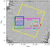Fig. 1 Footprints of VLA-VVDS (B03 field; in blue), SXDF (S06 field; in brown), VIDEO (in green), SERVS (in magenta), UDS (in cyan), SpUDS (in red), and SWIRE (in yellow) fields overplotted on our 325 MHz GMRT image. CFHTLS-D1 covers the same area as VLA-VVDS.

2. USS sample selection

2.1. 325 MHz GMRT observations of the XMM-LSS

We obtained 325 MHz GMRT observations of the XMM-LSS field over sky area of ~12 deg² with synthesized beamsize ~10.̋9. In the mosaiced 325 MHz GMRT image the average noise rms is ~160 μJy, while in the central region the average noise-rms reaches to ~120 μJy. Our 325 MHz observations are one of the deepest low-frequency surveys over such a wide sky area and detect ~2553/3304 radio sources at ≥5.0σ with noise rms cut-off ≤200/300 μJy. Since the local noise rms varies with distance from the phase center and also in the vicinity of bright sources, the rms map was used for source extraction and this approach helped to minimize the detection of spurious sources. We only consider sources with peak source brightness greater than 5 times the local rms noise value. The source position (right ascension and declination) is determined as the flux-density weighted centroid of all the emission enclosed within the 3σ contour. The typical error in the positions of the sources is about 1.4 arcsec and is estimated using the formalism outlined by Condon et al. (1998). The procedures opted for the data reduction and source extraction are similar to the 325 MHz GMRT observations of ELAIS-N1 presented in Sirothia et al. (2009). The details of our radio observations, data reduction, and source catalog of the XMM-LSS field will be presented in Sirothia et al. (in prep.). We note that our 325 MHz observations are ~5 times deeper than the previous 325 MHz observations of the XMM-LSS field (e.g., Tasse et al. 2006; Cohen et al. 2003), and result in similar manifold increase in the source density. Furthermore, our 325 MHz observations are ~3 times more sensitive (assuming typical spectral index for radio sources α ≃ −0.7) than the existing 610 MHz observations in the XMM-LSS (e.g., Tasse et al. 2007).

2.2. Other radio observations in the XMM-LSS field

The XMM-LSS field has been observed at different radio frequencies with varying sensitivities and sky area coverages (e.g., Bondi et al. 2003, 2007; Cohen et al. 2003; Simpson et al. 2006; Tasse et al. 2006, 2007). Among the deep surveys, there are 1.4 GHz and 610 MHz observations of 1.0 deg² in the VVDS field (Bondi et al. 2003, 2007) and 1.4 GHz observations of 1.3 deg² in the SXDF fields (Simpson et al. 2006). The 1.4 GHz VLA observations of 1.0 deg² in the VLA-VVDS field detect total ~1054 radio sources above the 5σ limit (~80 μJy) with resolution of ~6.0′′ (Bondi et al. 2003). The 610 MHz GMRT observations of the same area in the VLA-VVDS field detect total ~512 radio sources above 5σ limit (~250 μJy) with resolution of ~6.0′′ (Bondi et al. 2007). Simpson et al. (2006) present 1.4 GHz VLA observations of ~1.3 deg² in the SXDF field and detect ~512 sources over central ~0.8 deg² above 5σ detection limit (~100 μJy).

2.3. Cross-matching of 325 MHz sources and 1.4 GHz sources

We cross-match 325 MHz GMRT sources with 1.4 GHz VLA sources in the B03 and the S06 subfields and select our sample of USS sources based on 325 MHz to 1.4 GHz spectral index. To cross-match 325 MHz sources with 1.4 GHz sources we follow the method proposed by Sirothia et al. (2009). We identify 1.4 GHz counterparts of 325 MHz sources by using a search radius of 7.5 arcsec for unresolved sources and a larger search radius equal to the sum of half of the angular size and 7.5 arcsec for resolved sources. The value of the search radius is approximately equal to the sum of the half power synthesized beamwidths at 1.4 GHz and 325 MHz. We checked with increasing search radii from 7.̋5 to 10${}^{\mathrm{\prime }}\mathrm{\prime }^{\mathrm{\prime }}{}^{\mathrm{\prime }}$ and 15${}^{\mathrm{\prime }}\mathrm{\prime }^{\mathrm{\prime }}{}^{\mathrm{\prime }}$, and found that the number of unresolved cross-matched sources remains nearly same. Since the radio source density is low, i.e.,only 1054 sources detected at 1.4 GHz over 1.0 deg^-2, the chance coincidence in our cross-matching of 325 MHz sources to 1.4 GHz radio sources is rather small, i.e.,0.14%. The cross-matching of 325 MHz and 1.4 GHz radio source catalogs yields a total of 338 and 190 cross-matched sources in the B03 and the S06 subfields, respectively (see Table1). There are a large number of faint 1.4 GHz sources without 325 MHz counterparts and this can be understood as the 1.4 GHz observations are much deeper (~80–100 μJy at 5σ level) compared to the 325 MHz observations. However, the 5σ detection limit (~800 μJy) of our 325 MHz observations corresponds to ~288 μJy at 1.4 GHz, assuming a typical spectral index for radio sources (α) ~ − 0.7. Furthermore, there are a few 325 MHz detected radio sources that are not detected in the 1.4 GHz observations at ≥5.0σ. These sources can be explained if they have ultra steep spectral index ($\mathit{\alpha }\begin{array}{c}\mathrm{1.4}\mathrm{GHz}\\ \mathrm{325}\mathrm{MHz}\end{array}\mathrm{\le }\mathrm{-}\mathrm{1.3}$). We discuss these sources in the next section.

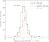Fig. 2 Histogram of 325 MHz to 1.4 GHz spectral index (${\mathit{\alpha }}_{\mathrm{325}\mathrm{MHz}}^{\mathrm{1.4}\mathrm{GHz}}$). Green solid line histogram represents sources in the B03 field while red dashed line histogram represents sources in the S06 field. Median spectral indices in the B03 field (${\mathit{\alpha }}_{\mathrm{325}\mathrm{MHz}\mathit{,}\mathrm{median}}^{\mathrm{1.4}\mathrm{GHz}}\mathrm{~}\mathrm{-}\mathrm{0.87}$) and in the S06 field (${\mathit{\alpha }}_{\mathrm{325}\mathrm{MHz}\mathit{,}\mathrm{median}}^{\mathrm{1.4}\mathrm{GHz}}\mathrm{~}\mathrm{-}\mathrm{0.76}$) are represented by vertical green dashed-dotted and red dashed lines, respectively. USS limit (${\mathit{\alpha }}_{\mathrm{325}\mathrm{MHz}}^{\mathrm{1.4}\mathrm{GHz}}\mathrm{\le }\mathrm{-}\mathrm{1}$) is represented by the vertical dotted line.

2.4. 325 MHz–1.4 GHz radio spectral index

We estimate the radio spectral index (α, where S_ν ∝ ν^α) for all the sources that are detected at both 325 MHz and 1.4 GHz frequencies. Figure 2 shows the histograms of spectral index of cross-matched sources for both the B03 and the S06 fields. The median values of the spectral index distributions ($\mathit{\alpha }\begin{array}{c}\mathrm{1.4}\mathrm{GHz}\\ \mathrm{325}\mathrm{MHz}\end{array}$) are –0.86 (standard deviation ~0.38) and –0.76 (standard deviation ~0.40) in the B03 and the S06 fields, respectively. The higher median spectral index in the B03 field is possibly due to the deeper 1.4 GHz source catalog, i.e.,faint 1.4 GHz sources with steeper spectral index are favored to be detected at 325 MHz. Figure 3 shows the 1.4 GHz flux density versus spectral index ($\mathit{\alpha }\begin{array}{c}\mathrm{1.4}\mathrm{GHz}\\ \mathrm{325}\mathrm{MHz}\end{array}$) plot. The differing sensitivities at the two frequencies result in a bias against flat spectral index sources, i.e.,faint 1.4 GHz sources with relatively flat spectral index have corresponding 325 MHz flux density below the detection limit of less sensitive 325 MHz observations. The large number of sources lying along the 325 MHz flux density limit line in the spectral index versus flux density plot reflects the fact that 1.4 GHz observations are deeper than 325 MHz observations.

2.5. USS sample

In the literature there is no uniform definition for a USS source and different studies have used different frequencies and different spectral index thresholds e.g.,${\mathit{\alpha }}_{\mathrm{151}\mathrm{MHz}}^{\mathrm{4.85}\mathrm{GHz}}\mathrm{\le }\mathrm{-}\mathrm{0.9}$81 (Blundell et al. 1998), ${\mathit{\alpha }}_{\mathrm{74}\mathrm{MHz}}^{\mathrm{325}\mathrm{MHz}}\mathrm{\le }\mathrm{-}\mathrm{1.}$2 (Cohen et al. 2004), ${\mathit{\alpha }}_{\mathrm{408}\mathrm{MHz}}^{\mathrm{843}\mathrm{MHz}}\mathrm{\le }\mathrm{-}\mathrm{1}$.3 (De Breuck et al. 2004), ${\mathit{\alpha }}_{\mathrm{151}\mathrm{MHz}}^{\mathrm{1.4}\mathrm{GHz}}\mathrm{\le }\mathrm{-}\mathrm{1.}$0 (Cruz et al. 2006), ${\mathit{\alpha }}_{\mathrm{408}\mathrm{MHz}}^{\mathrm{843}\mathrm{MHz}}\mathrm{\le }\mathrm{-}\mathrm{1.}$0 (Broderick et al. 2007), and ${\mathit{\alpha }}_{\mathrm{150}\mathrm{MHz}}^{\mathrm{1.4}\mathrm{GHz}}\mathrm{\le }\mathrm{-}\mathrm{1}$.0 (Ishwara-Chandra et al. 2010). To select our sample of USS sources we use spectral index cut-off ${\mathit{\alpha }}_{\mathrm{325}\mathrm{MHz}}^{\mathrm{1.4}\mathrm{GHz}}\mathrm{\le }\mathrm{-}\mathrm{1.}$0 (spectra steeper than –1.0). The spectral index may change with frequency because of spectral curvature (Bornancini et al. 2007), although most of HzRGs show linear spectra over a large frequency range (Klamer et al. 2006). Thus, a higher cut-off in the spectral index at 325 MHz will translate into even higher cut-off at the rest frame if a source exhibits spectral steepening at higher frequencies. Furthermore, at fainter flux densities, the less luminous radio sources can have marginally flatter spectra because of the observed correlation between the radio power and the spectral index, i.e.,the P − α relation (Mangalam & Gopal-Krishna 1995; Blundell et al. 1999). Since we are studying faint USS sources to identify HzRGs there is a possibility that a large fraction of HzRGs may be missed if we adopt a very steep spectral index cut-off (e.g., α ≤ −1.3). Moreover, if we happen to pick up low redshift sources in our USS sample by using a less steep spectral index cut-off, these sources are likely to have optical counterparts and redshift estimates, and therefore can be identified and eliminated. Using the spectral index $\mathit{\alpha }\begin{array}{c}\mathrm{1.4}\mathrm{GHz}\\ \mathrm{325}\mathrm{MHz}\end{array}\mathrm{\le }\mathrm{-}\mathrm{1.}$0 for a source to be classified as USS source in the 325 MHz–1.4 GHz cross-matched catalogs, we obtain 111 and 39 USS sources in the B03 and S06 fields, respectively (see Table 1).

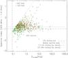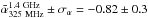
Fig. 3 Spectral index (${\mathit{\alpha }}_{\mathrm{325}\mathrm{MHz}}^{\mathrm{1.4}\mathrm{GHz}}$) versus 1.4 GHz flux density plot. Plus (+) and cross (×) symbols represent USS sources in the B03 and in the S06 fields, respectively. The dashed line represents the median spectral index value (${\mathit{\alpha }}_{\mathrm{325}\mathrm{MHz}}^{\mathrm{1.4}\mathrm{GHz}}\mathrm{~}\mathrm{-}\mathrm{0.83}$) for the full sample. The flux density limits at 325 MHz and 1.4 GHz are represented by dotted and long-dashed lines, respectively.

There are five radio sources in each subfield that are detected in 325 MHz at ≥5σ, but do not have 1.4 GHz counterpart at ≥5σ flux limit. These sources are potential faint USS sources; because of their very steep spectral index they are detected above 5σ at 325 MHz, but fall below 5σ detection at 1.4 GHz. To find the 1.4 GHz counterparts of such sources we inspected 1.4 GHz images and find that all sources are detected between 3σ and 5σ. We obtained their 1.4 flux densities by fitting the source with an elliptical Gaussian using the task JMFIT in AIPS¹. It turns out that some of these sources are marginally resolved with peak flux density below 5σ while total flux density is above 5σ. Thus, the resultant spectral index is not as steep as expected from the 5σ detection flux limit at 1.4 GHz. The addition of these USS sources (detected above 5σ at 325 MHz, but falling below 5σ at 1.4 GHz) to those detected at ≥5σ in both frequencies yield, in total, 116 and 44 USS sources in the B03 and the S06 fields, respectively, and a full sample of 160 USS sources (see Table 1). The flux density measurement errors give rise to uncertainties in spectral indices and this could result in scattering of some non-USS sources into the USS sample and vice-versa. In order to statistically quantify the contamination of non-USS sources into the USS sample, we consider spectral index distribution of 325 MHz selected sources described by a normal distribution of $\mathit{\alpha ̅}\begin{array}{c}\mathrm{1.4}\mathrm{GHz}\\ \mathrm{325}\mathrm{MHz}\end{array}\mathrm{\pm }{\mathit{\sigma }}_{\mathit{\alpha }}\mathrm{=}\mathrm{-}\mathrm{0.82}\mathrm{\pm }\mathrm{0.3}$9, and the distributions of errors on spectral indices described by a normal distribution of Δα ± σ_Δα = 0.08 ± 0.05. As our spectral index cut-off for USS sources $\mathit{\alpha }\begin{array}{c}\mathrm{1.4}\mathrm{GHz}\\ \mathrm{325}\mathrm{MHz}\end{array}\mathrm{=}\mathrm{-}\mathrm{1.}$0 lies at the steep tail of the spectral index distribution, a higher number of non-USS sources $\mathit{\alpha }\begin{array}{c}\mathrm{1.4}\mathrm{GHz}\\ \mathrm{325}\mathrm{MHz}\end{array}\mathit{>}\mathrm{-}\mathrm{1.0}$ are expected to scatter into the USS sample than the USS sources scatter to non-USS regime. Using the median uncertainty of spectral indices and a normal distribution for spectral indices we find that 48 non-USS sources with observed spectral index $\mathit{\alpha }\begin{array}{c}\mathrm{1.4}\mathrm{GHz}\\ \mathrm{325}\mathrm{MHz}\end{array}\mathit{>}\mathrm{-}\mathrm{1.}$0 may have intrinsic spectral index $\mathit{\alpha }\begin{array}{c}\mathrm{1.4}\mathrm{GHz}\\ \mathrm{325}\mathrm{MHz}\end{array}\mathrm{\le }\mathrm{-}\mathrm{1.0}$, while 43 USS sources with observed spectral index $\mathit{\alpha }\begin{array}{c}\mathrm{1.4}\mathrm{GHz}\\ \mathrm{325}\mathrm{MHz}\end{array}\mathrm{\le }\mathrm{-}\mathrm{1.0}$ may have intrinsic spectral index $\mathit{\alpha }\begin{array}{c}\mathrm{1.4}\mathrm{GHz}\\ \mathrm{325}\mathrm{MHz}\end{array}\mathit{>}\mathrm{-}\mathrm{1.0}$. This indicates that the contamination by non-USS sources in our sample can be as large as 48/160 ~ 30%. The contamination by intrinsically non-USS sources is likely to result in the increase of low-z sources in our USS sample.

2.6. Comparison with the 610 MHz–1.4 GHz USS sample

Bondi et al. (2007) present a sample of 58 faint USS sources (${\mathit{\alpha }}_{\mathrm{610}\mathrm{MHz}}^{\mathrm{1.4}\mathrm{GHz}}\mathrm{\le }\mathrm{-}\mathrm{1.3}$) using deep 1.4 GHz (5σ ~ 80μJy) and 610 MHz (5σ ~ 250μJy) observations of 1.0 deg^-2 in the VLA-VVDS field. 39/58 of these USS sources have 1.4 GHz detection at ≥5σ and 610 MHz detection at ≥3σ, while the rest of the 19/58 USS sources have 610 MHz detection at ≥5σ, but the 1.4 GHz detection is between 3σ and 5σ. We derive our USS sample (${\mathit{\alpha }}_{\mathrm{325}\mathrm{MHz}}^{\mathrm{1.4}\mathrm{GHz}}\mathrm{\le }\mathrm{-}\mathrm{1.0}$) in the same field using low-frequency 325 MHz observations and 1.4 GHz observations. We find that only 11 USS sources are common to our USS sample (${\mathit{\alpha }}_{\mathrm{325}\mathrm{MHz}}^{\mathrm{1.4}\mathrm{GHz}}\mathrm{\le }\mathrm{-}\mathrm{1.0}$) and the USS sample of Bondi et al. (2007) (${\mathit{\alpha }}_{\mathrm{610}\mathrm{MHz}}^{\mathrm{1.4}\mathrm{GHz}}\mathrm{\le }\mathrm{-}\mathrm{1.3}$). The mismatch could be attributed to different flux limits as we have considered only those sources that are detected at ≥5σ at both 1.4 GHz and 325 MHz. Bondi et al. (2007) cautioned that all 58 of their USS candidates are weak radio sources (i.e.,50 μJy ≤ S_{1.4 GHz} ≤ 327 μJy, with the median S_{1.4 GHz} ~ 90μJy), and therefore errors in the total flux density determination can be relatively large, yielding to a less secure spectral index value. Since USS sources are faint and unresolved, we used peak flux densities and find that 22/58 USS sources have extrapolated 325 MHz flux density below the detection limit of our GMRT observations (i.e.,S_{325 MHz}< 0.80 μJy). The non-detection of the rest of the 25/58 sources at 325 MHz can be explained if these sources exhibit spectral turnover between 325 MHz to 610 MHz, or if there is large uncertainty associated with the 610 MHz–1.4 GHz spectral index (${\mathit{\alpha }}_{\mathrm{610}\mathrm{MHz}}^{\mathrm{1.4}\mathrm{GHz}}$). The possibility of some of the sources being similar to gigahertz peaked sources or affected by variability cannot be ruled out. For the rest of the 105 USS sources (${\mathit{\alpha }}_{\mathrm{325}\mathrm{MHz}}^{\mathrm{1.4}\mathrm{GHz}}\mathrm{\le }\mathrm{-}\mathrm{1.0}$) of our sample, 80, 16, and 9 sources have 610 MHz detection at ≥5σ, 3σ − 5σ, and <3σ, respectively. Most of our USS sources (${\mathit{\alpha }}_{\mathrm{325}\mathrm{MHz}}^{\mathrm{1.4}\mathrm{GHz}}\mathrm{\le }\mathrm{-}\mathrm{1.0}$) have ${\mathit{\alpha }}_{\mathrm{610}\mathrm{MHz}}^{\mathrm{1.4}\mathrm{GHz}}\mathrm{~}\mathrm{-}\mathrm{1.3}$ to −0.7, which is consistent within uncertainties.

3. The optical, near-IR, and mid-IR counterparts of USS sources

To characterize the nature of our USS radio sources we study the properties of their counterparts in different bands at optical and IR wavelengths.

3.1. The optical, near-IR, and mid-IR data

The B03 field:

to find the optical counterparts of our USS sources, we use VLT VIMOS Deep Survey (VVDS²) and Canada-France-Hawaii Telescope Legacy Survey (CFHTLS³) D1 photometric data. Ciliegi et al. (2005) present optical identification of 1.4 GHz radio sources using VVDS photometric data in B, V, R, and I bands. In near-IR, we use VISTA Deep Extragalactic Observations (VIDEO; Jarvis et al. 2013) survey which provides photometric observations in Z, Y, J, H, and Ks bands and covers full 1.0 deg^-2 of the B03 field. McAlpine et al. (2013) cross-matched 1.4 GHz radio sources to the K-band VIDEO data and also used CFHTLS-D1 photometric data in u^⋆, g′, r′, i′, and z′ bands along with VIDEO photometric data to obtain photometric redshift estimates of 1.4 GHz radio sources. To find mid-IR counterparts we use Spitzer Extragalactic Representative Volume Survey (SERVS) data (Mauduit et al. 2012). SERVS is a medium deep survey at 3.6 and 4.5 μm and has partial overlap of ~0.82 deg^-2 with the B03 field (see Fig. 1).

The S06 field:

Simpson et al. (2006) present optical identifications of 1.4 GHz radio sources using the Subaru/Suprime-Cam observations in B, V, R, i′, and z′ bands. To find the optical counterparts of our USS sources we use optical radio cross-matched catalog of Simpson et al. (2006). In near-IR, we use the Ultra Deep Survey⁴ (UDS) DR8 from the UKIRT Infrared Deep Sky Survey (UKIDSS, Lawrence et al. 2007) which has ~0.63 deg^-2 of overlap with the S06 field. The mid-IR counterparts are found using the Spitzer Public Legacy Survey of the UKIDSS Ultra Deep Survey (SpUDS⁵; Dunlop et al. 2007) which is carried out with all four IRAC bands (3.6, 4.5, 5.8 and 8.0 μm), and one MIPS band (24 μm).

3.2. The optical, near-IR, and mid-IR identification rates

Table 2 lists the identification rates, medians, and standard deviations of the optical, near-IR, and mid-IR magnitude distributions for our USS sample sources as well as for the full radio population in the two subfields. The optical, near-IR, and mid-IR counterparts of radio sources are found using the likelihood ratio method and only counterparts with high reliability are considered as true counterparts (e.g., Ciliegi et al. 2005; Simpson et al. 2006; McAlpine et al. 2013). We visually inspected near-IR/mid-IR images (e.g.,from VIDEO, UDS, SERVS, and SpUDS imaging) at the positions of all the USS sources and ensure that the counterparts found using the likelihood method are correct. The visual inspection at the positions of non-detections (i.e.,the USS sources without counterparts) shows that the most of these sources remain undetected, except a few with either tentative faint counterparts below 5σ or lying close to a bright source. Furthermore, the cross-matching of optical/near-IR/mid-IR sources with the 1.4 GHz radio sources shifted in random directions with random distances in the range of 30–45 arcsec yields only ~2–4% counterparts. This indicates that the false identification rate is limited only to a few percent.

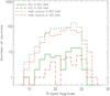Fig. 4 Histograms of R-band magnitudes of the USS sources and of the full 1.4 GHz radio population in the B03 and the S06 field. Histograms of USS sources are shown by green solid lines and red long dashed lines for the B03 and the S06 fields, respectively. While green dashed and red dashed-dotted lines represent histograms for the full 1.4 GHz radio population in the B03 and the S06 fields, respectively.

From Table 2 it is evident that less deep optical/near-IR/mid-IR surveys in the B03 field (i.e.,Ks_AB ≤ 23.8) yields a lower identification rate for USS sources (~74%) compared to that for the full radio population (~89%). While the use of deeper optical/near-IR/mid-IR data in the S06 field yields high and nearly similar identification rates (i.e.,92%) for both USS and for the full radio population. Previous studies have shown that the identification rates of bright USS sources with the optical/near-IR surveys limited to brighter magnitudes yield lower identification rates (Wieringa & Katgert 1991; Intema et al. 2011). However, deeper surveys result in high identification rates for both USS and non-USS sources (De Breuck et al. 2002a; Afonso et al. 2011). Thus, our results on the optical/near-IR/mid-IR identification rates of our faint USS sources using existing deep surveys are consistent with previous findings.

Figures 4–6, respectively, show R band, K band, and 3.6 μm magnitude distributions of our USS sources and of the full radio population, for both the subfields. We note that the optical/near-IR/mid-IR magnitude distributions of USS sources are flatter and have higher medians compared to the ones for the full radio population. This suggests that optical/near-IR/mid-IR counterparts of USS sources are systematically fainter compared to the ones for non-USS radio population. The two sample Kolmogorov-Smirnov (KS) test shows that the difference between the magnitude distributions of our USS sources and the full radio population increases at redder bands. The probability that null hypothesis is true, i.e.,the two samples have same distributions, decreases in red and IR bands (see Table 2). The two sample KS test on the comparison of the magnitude distributions of USS and non-USS radio sources give similar results. Thus, the comparison of optical/near-IR/mid-IR magnitude distributions of our USS sources and the full radio population is consistent with the interpretation that USS sources are fainter and sample high-z and/or dusty sources that have higher chances of being detected in the red/IR bands.

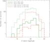Fig. 5 Histograms of K-band magnitudes of the USS sources and of the full 1.4 GHz radio population in the B03 and the S06 field. Histograms of USS sources are shown by green solid lines and red long dashed lines for the B03 and the S06 fields, respectively. Green dashed and red dashed-dotted lines represent histograms for the full 1.4 GHz radio population in the B03 and the S06 fields, respectively.

4. Redshift distributions

To obtain redshifts of our USS sample sources, we use the spectroscopic and photometric measurements available in the literature.

The B03 field:

there has been more than one attempt to estimate photometric redshifts of the 1.4 GHz radio sources in the B03 field (e.g., Ciliegi et al. 2005; Bardelli et al. 2009; McAlpine et al. 2013). Using deep ten-band photometric data (i.e.,five bands of near-IR VIDEO data combined with five bands of CFHTLS-D1 optical data) McAlpine et al. (2013) present the most accurate photometric redshift estimates of 1.4 GHz radio sources. The photometric redshifts were determined using the code Le Phare⁶ (Ilbert et al. 2006) that uses a trial of fitting the photometric bands with a set of input spectral energy distribution (SED) templates. The accuracy of the photometric redshifts was assessed by comparing with secure spectroscopic redshifts obtained with the VIMOS VLT deep survey (VVDS; Le Fèvre et al. 2005). Approximately 3.8 per cent of the sources are catastrophic outliers, defined as cases with Δz/ (1 + z_s) > 0.15, where Δz = | z_p − z_s |. The details of the procedure used to derive these photometric redshifts are given in Jarvis et al. (2013).

Using photometric redshift estimates from McAlpine et al. (2013), we find that 86/116 USS sources in the B03 field have photometric redshifts. Nearly 0.64 deg² of the B03 field is also covered by the VVDS which is a magnitude limited spectroscopic redshift survey conducted by the VIMOS multi-slit spectrograph at the ESO-VLT (Le Fèvre et al. 2013). Using the latest VVDS catalog⁷, we find that only 11 USS sources have spectroscopic redshifts, and all these sources also have photo-z estimates from McAlpine et al. (2013). There are 30/116 (~25.8%) USS sources without redshift estimates and these may potentially be high redshift candidates that are too faint to be detected in existing optical and IR surveys.

The S06 field:

Simpson et al. (2012) present spectroscopic and 11−band (u^⋆, B, V, R, i′, z′, J, H, K plus IRAC bands 1 and 2) photometric redshifts for 505/512 1.4 GHz radio sources. The spectroscopic redshift measurements are obtained using the Visible Multi-Object Spectrograph (VIMOS) on the VLT and also include measurements from different spectroscopic campaigns in the SXDF field (e.g., Geach et al. 2007; Smail et al. 2008; van Breukelen et al. 2009; Banerji et al. 2011; Chuter et al. 2011). Spectroscopic redshifts are available for 267/505 radio sources, while the rest of the radio sources have photometric redshift estimates. The photometric redshifts were estimated using the code EAZY (Brammer et al. 2008) after correcting the observed photometry for Galactic extinction of A_V = 0.070 (Schlegel et al. 1998) with the Milky Way extinction law of Pei (1992). Using Simpson et al. (2012) redshifts measurements we find that spectroscopic redshifts are available for 16/44 USS sources, while 23/44 USS sources have photometric redshifts. We compare the spectroscopic redshifts (z_spec) and the photometric redshifts (z_phot) for all those USS sources that have both types of redshift estimates. Figure 7 shows the comparison of z_spec and z_phot and it is clear that the z_phot estimates are fairly consistent with the z_spec measurements at z ≤ 1.5. They are less accurate at higher redshifts. We do not see any catastrophic outliers in the comparison of spectroscopic redshifts (z_spec) and photometric redshifts (z_phot), although this comparison is limited only to a small fraction of our USS sources.

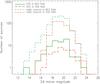Fig. 6 Histograms of 3.6 μm magnitudes of the USS sources and of the full 1.4 GHz radio population in the B03 and S06 field. Histograms of USS sources are shown by green solid lines and red long dashed lines for the B03 and the S06 fields, respectively. Green dashed and red dashed-dotted lines represent histograms for full 1.4 GHz radio population in the B03 and the S06 fields, respectively.

Figure 8 shows the redshift distributions of our USS sources in the two subfields. We use spectroscopic redshifts whenever available, otherwise photometric redshifts are used. The USS redshift distribution in the B03 field spans from 0.096 to 3.86 with mean (z_mean) ~1.31 and median (z_median) ~ 1.18. It is evident that substantially large fraction (53/86 ~ 61.5/ %) of USS sources in the B03 field, are lying at z ≥ 1.0. The USS redshift distribution in the S06 field is flatter and spans from 0.033 to 3.34 with z_mean ~ 1.54 and z_median ~ 1.57. We note that 27/44 ≃ 61.4% of USS sources in the S06 field are at redshifts (z) ≥ 1.0. The lower median redshift of the USS sample in the B03 field can be attributed to the fact that there are no redshift estimates for a significantly large fraction (30/116 ~ 25.8%) of USS sources in this field. The USS sources without redshifts remained undetected in the existing optical and IR surveys, and may possibly be faint sources at higher redshifts. We discuss the possible nature of these USS sources in the Sect. 5.2.

The USS redshift distribution in the B03 field also shows peaks at z ~ 0.3, z ~ 1.2 and at z ~ 1.5. It is to be noted that the redshift distribution of near-IR identified radio sources also exhibits peak at z ~ 0.2−0.4 and z ~ 1.0–1.2 (McAlpine et al. 2013). The redshift peak at z ~ 0.2–0.4 can plausibly be due to large-scale structure within this relatively small field, i.e.,there are six known X-ray clusters at z ≃ 0.262, 0.266, 0.293, 0.301, 0.307, and 0.345 (Pacaud et al. 2007; Adami et al. 2011) present in this field, which is at least partially responsible for an increase in the sources in this redshift range. We surmise that the redshift peaks at z ~ 1.2 and 1.5 may also be due to the presence of clusters at these redshifts, although we caution that most of redshift estimates are based on photometry.

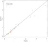Fig. 7 Comparison between the spectroscopic and the photometric redshifts of the USS sources in the B03 field (green circles) and in the S03 field (red squares). The diagonal line represents zspec = zphot.

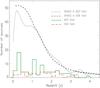Fig. 8 Redshift distributions of our USS sources in the B03 field (in green solid lines) and in the S06 field (in red dashed lines). Redshift estimates are available for 86/116 and 39/44 USS sources in the B03 field and the S06 field, respectively. The redshift distributions of 1.4 GHz radio population predicted by SKA simulated skies (SKADS; Wilman et al. 2008, 2010) for the B03 and the S06 fields are plotted with dotted and dashed curves, respectively. The flux limit S1.4 GHz ~ 100 μJy and sky area of 1.0 deg-2 in the B03 field and 0.8 deg-2 in the S06 field are used to obtain simulated radio populations for the two subfields, respectively. The redshift distributions of simulated radio populations in the B03 and the S06 fields are presented in McAlpine et al. (2013) and Simpson et al. (2012), respectively. The uneven variations seen in the SKADS simulated redshift distribution in the B03 field can be attributed to the clustering of radio sources manifested as cosmic variance in this relatively small field.

In order to examine whether our USS sample actually selects high-z sources, we compare median redshift of our USS sources with that of the non-USS sources. The 325 MHz−1.4 GHz cross-matched catalog yields 227 and 152 non-USS sources (${\mathit{\alpha }}_{\mathrm{325}\mathrm{MHz}}^{\mathrm{1.4}\mathrm{GHz}}\mathit{<}\mathrm{1.}$0) in the B03 and the S06 field, respectively. We find that only 192/227 (~84.6%) and 135/152 (~88.8%) do have redshift estimates with the median redshift values ~0.99 and ~0.96, in the B03 and the S06 field, respectively. It is evident that on average the USS sources (z_median ~ 1.18 in the B03 field and z_median ~ 1.57 in the S06 field) are at higher redshifts than the non-USS radio sources. To check, if within the USS sample, the radio sources with much steeper spectral index are at much higher redshifts, we make two subsamples of USS sources, i.e.,one consists of sources with ${\mathit{\alpha }}_{\mathrm{325}\mathrm{MHz}}^{\mathrm{1.4}\mathrm{GHz}}\mathrm{\le }\mathrm{-}\mathrm{1.}$3, and the other USS subsample consists of sources with $\mathrm{-}\mathrm{1.3}\mathit{<}{\mathit{\alpha }}_{\mathrm{325}\mathrm{MHz}}^{\mathrm{1.4}\mathrm{GHz}}\mathrm{\le }\mathrm{-}\mathrm{1}$.0. We find that, in the B03 field, among the 86/116 sources with available redshifts only 22/86 USS sources have ${\mathit{\alpha }}_{\mathrm{325}\mathrm{MHz}}^{\mathrm{1.4}\mathrm{GHz}}\mathrm{\le }\mathrm{-}\mathrm{1.}$3 and yield median redshift of ~1.72, while 64/86 USS sources with $\mathrm{-}\mathrm{1.3}\mathit{<}{\mathit{\alpha }}_{\mathrm{325}\mathrm{MHz}}^{\mathrm{1.4}\mathrm{GHz}}\mathrm{\le }\mathrm{-}\mathrm{1}$.0 have median redshift of ~1.08. In the S06 field, among the 39/44 USS sources with available redshifts only 5 USS sources have ${\mathit{\alpha }}_{\mathrm{325}\mathrm{MHz}}^{\mathrm{1.4}\mathrm{GHz}}\mathrm{\le }\mathrm{-}\mathrm{1}$.3 with the median redshift ~1.32, while 34 USS sources with $\mathrm{-}\mathrm{1.3}\mathit{<}{\mathit{\alpha }}_{\mathrm{325}\mathrm{MHz}}^{\mathrm{1.4}\mathrm{GHz}}\mathrm{\le }\mathrm{-}\mathrm{1.}$0 have median redshift ~1.57. It is to be noted that, in the S06 field, the number of USS sources with ${\mathit{\alpha }}_{\mathrm{325}\mathrm{MHz}}^{\mathrm{1.4}\mathrm{GHz}}\mathrm{\le }\mathrm{-}\mathrm{1.}$3 is not sufficient to make a robust statistical comparison. Therefore, based on the USS sources in the B03 field, we find that, on average, sources with steeper radio spectral index tend to have higher redshift. This result is consistent with the z − α correlation (Ker et al. 2012).

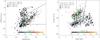Fig. 9 Mid-IR color–color diagnostic plots for our USS sources in both the B03 and S06 fields. Left and right panels show mid-IR color–color plots based on Lacy et al. (2004) and Stern et al. (2005) criteria, respectively. Filled and open symbols represent USS sources and 1.4 GHz radio populations, respectively. USS sources of different redshifts are shown with different colors. The regions bounded by dashed lines denotes AGN selection wedge. Lacy et al. (2004) defined the AGN selection wedge as: (log(S5.8/S3.6) > −0.1) ∧ (log(S8.0/S4.5) > −0.8) ∧ (log(S8.0/S4.5) ≤ 0.8 log(S5.8/S3.6) + 0.5); where ∧ is “AND” operator. While, the AGN selection wedge proposed by Stern et al. (2005) is defined as: ([5.8] – [8.0] > 0.6) ∧ ([3.6] – [4.5] > 0.2([5.8] – [8.0]) + 0.18) ∧ ([3.6] – [4.5 ] > 2.5 ([5.8]–[8.0]) – 3.5); where IRAC magnitudes are in the Vega system. We converted IRAC AB magnitudes to Vega magnitudes (mAB = mVega + conv) using conversion factors 2.78, 3.26, 3.75, and 4.38 for 3.6 μm, 4.5 μm, 5.8 μm, and 8.0 μm bands, respectively (see IRAC Data HandBook 3.0 2006).

We also compare the redshift distribution of our USS sources with the one for the radio population derived by using the SKADS Simulated Skies (S³) simulations (Wilman et al. 2008, 2010) (see Fig. 8). The S³ simulation uses a model that includes different radio populations, i.e.,star-forming galaxies, radio-quiet AGNs, radio-loud AGNs (FR−I and FR−II radio galaxies). The S³-simulations⁸ do not cover 325 MHz frequency which is the base frequency of our USS sample, and therefore we use 1.4 GHz frequency to obtain the redshift distribution of the simulated radio population. Figure 8 shows that the redshift distributions of the simulated 1.4 GHz radio populations peak at low redshift with a sharp decline over z ~ 1 to 3 and a nearly flat tail at z > 3.0. In contrast to the simulated radio population, the redshift distributions of USS sources in the two subfields are nearly flat, except for the two peaks seen in the B03 field that are possibly attributed to the presence of galaxy clusters in this field. The difference between the redshift distributions of USS sources and the simulated radio population is maximum at low redshift, while it decreases at higher redshifts, particularly at z ≥ 2.0. This suggests that the USS technique preferentially selects high-z sources, while removing a large fraction of low-z sources. At sub-mJy flux densities, the radio population is known to be dominated by star-forming galaxies and low-power AGNs with increasing contribution by AGNs at higher redshifts (Wilman et al. 2008, 2010). Thus, in our faint USS sample, the high-z radio sources are likely to be dominated by relatively low-power AGNs such as FR−I radio galaxies. However, powerful FR−II radio galaxies at even higher redshifts can also be present in our USS sample.

5. Color−color diagnostics

In order to understand the nature of USS sources in our sample we investigate the mid-IR colors and the flux ratios of radio to mid-IR.

5.1. Mid-IR colors

Mid-IR Spectral Energy Distributions (SEDs) of AGN are generally characterized by a power law and differ from star-forming galaxies (Alonso-Herrero et al. 2006; Donley et al. 2007). Therefore, mid-IR colors are useful in identifying the presence of AGN-heated dust in the SEDs of galaxies. We investigate the nature of our USS sample sources using mid-IR color diagnostics proposed by Lacy et al. (2004) and Stern et al. (2005). We note that only 32/116 (27.6%) USS sources in the B03 field and 32/44 (72.7%) USS sources in the S06 field have detections in all four IRAC bands (3.6, 4.5, 5.8, and 8.0 μm) from the SWIRE and the SpUDS data, respectively. Thus, the mid-IR color–color diagnostic is limited only to a fraction of our USS sample sources. The higher fraction of USS sources detected in the S06 field may be attributed to the deeper SpUDS data (5σ depth at 3.6 μm ~ 0.9 μJy) compared to the SWIRE (5σ depth at 3.6 μm ~ 3.7 μJy).

Figure 9 shows mid-IR color–color diagnostic plots for our USS sample sources as well as for the radio population in the two subfields. The mid-IR color–color diagnostic plots based on Lacy et al. (2004) and Stern et al. (2005) criteria show that our USS sources exhibit a wide range of mid-IR colors with large fraction of USS sources falling in the AGN selection wedge. However, in the B03 field, nearly half of the USS sample sources reside outside the AGN selection wedge. Notably, most of the USS sources lying outside of the AGN wedge selection are of low redshifts (z ≤ 0.5). Therefore, low-z USS sources of our sample, particularly in the B03 field, are likely to be contaminated by star-forming galaxies or composite galaxies in which IR emission is dominated by star formation. We note that our mid-IR color diagnostic, in the B03 field, is based on the relatively shallow SWIRE data which is expected to detect relatively bright sources. The USS sources at higher redshifts (z > 0.5), in both the subfields, preferentially fall either inside or close to the AGN selection wedge. Thus, mid-IR color–color diagnostics are consistent with a large fraction of our USS sample sources at higher redshifts (z > 0.5) being mainly AGN. However, because of non-detection of a substantial fraction of USS sources in all four IRAC bands, we cannot obtain the exact fraction of AGN dominated USS sources in our sample. Furthermore, we caution that the mid-IR color–color diagnostic plots are known to be contaminated, i.e.,AGN may fall in non-AGN regions and vice-versa (see Donley et al. 2008, 2012; Barmby et al. 2008). The samples of radio-loud AGN are known to exhibit a wide variety of IR colors with dichotomy displayed in mid-IR-radio plane for low and high excitation radio galaxies (see Gürkan et al. 2014). There are suggestions that radio selected AGNs may have different accretion mode, i.e.,radiatively inefficient (radio mode), and may not strictly follow the mid-IR color selection criteria (Croton et al. 2006; Hardcastle et al. 2007; Tasse et al. 2008; Griffith & Stern 2010).

Simpson et al. (2012) present optical spectra of 267/512 radio sources detected at 1.4 GHz in the S06 field. Our USS sources are a subsample of the 1.4 GHz radio sources and we find that optical spectra are available for 15 USS sources. Spectral classifications based on observed emission and/or absorption line properties show that five USS sources are narrow-line AGN (NLAGN), five USS sources are star burst (SB), three and one USS sources are, respectively, strong and weak line emitters with uncertain classification, and one source is classified as absorption line galaxy. We note that the USS sources classified as starburst galaxies are preferentially at lower redshifts (z< 0.5), while NLAGNs are at higher redshifts (z> 0.5), which is consistent with the findings of our mid-IR color–color diagnostic.

5.2. Flux ratios of radio to mid-IR

The ratio of 1.4 GHz flux density to 3.6 μm flux (S_{1.4 GHz}/S_{3.6 μm}) versus redshift plot can be used as a diagnostic to differentiate sources of different classes, i.e.,star-forming galaxies, radio-quiet AGN, HzRGs (see Norris et al. 2011a). In general, HzRGs and radio-loud AGNs exhibit a high ratio of 1.4 GHz flux density to 3.6 μm flux (S_{1.4 GHz}/S_{3.6 μm}), while radio-quiet and star-forming galaxies are characterized by a low ratio. Figure 10 shows the ratio of 1.4 GHz flux density to 3.6 μm flux (S_{1.4 GHz}/S_{3.6 μm}) versus redshift plot for our USS sample sources. We note that the radio to mid-IR flux ratio diagnostic is limited only to those USS sources that are covered by SERVS (e.g.,95/116 USS in the B03 field) and SpUDS (e.g.,36/44 USS in the S06 field) survey regions (see Fig. 1). In our sample, 72/95 USS sources in the B03 field and 32/36 USS sources in the S06 field do have a 3.6 μm counterpart (see Table 2). While, for USS sources without 3.6 μm detections (i.e.,16 sources in the B03 field and four sources in the S06 field), we put a lower limit on the flux ratio S_{1.4 GHz}/S_{3.6 μm} using 3.6 μm survey flux limits (i.e.,2.0 μJy for the SERVS data and 0.9 μJy for the SpUDS data). We note that in the B03 field there are seven USS sources with extended radio sizes for which 3.6 μm counterparts are unavailable because of ambiguity caused by the existence of more than one IRAC source detected within their radio sizes. These sources are not included in the flux ratio diagnostic plot.

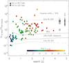Fig. 10 Ratio of 1.4 GHz radio flux density to 3.6 μm flux (S1.4 GHz/S3.6 μm) versus redshift plot for our USS sources. USS sources of different radio luminosities are represented with different colors. USS sources without redshift estimates are shown at the rightmost position. USS sources with only lower limits on the flux ratios (S1.4 GHz/S3.6 μm), i.e.,without 3.6 μm detections, are shown by upward arrows. The area above the dotted line represents the range of flux ratios for the powerful HzRGs and IFRSs. Tracks indicating the regions for the different classes of sources are taken from Norris et al. (2011a). The solid lines represent the loci of LIRGs and ULIRGs using Rieke et al. (2009) SED templates. The dashed (long dashed) line indicates the loci of radio-loud (radio-quiet) QSOs from Elvis et al. (1994). We caution that dust extinction can cause any of these tracks to rise steeply at high redshift where the observed 3.6 μm is emitted in visible wavelengths at the rest frame.

From Fig. 10, it is evident that our USS sample sources in both the subfields are distributed over a wide range of flux ratios (S_{1.4 GHz}/S_{3.6 μm} ~ 0.1–1000) and redshifts (z ~ 0.1 − 3.8). The flux diagnostic plot also shows tracks indicating regions of different classes of sources as proposed by Norris et al. (2011a). From the flux diagnostic plot, it is clear that our USS sample contains sources of various classes. At low redshifts (z ≤ 0.5), most of our USS sources tend to exhibit a low ratio of radio to mid-IR (i.e.,S_{1.4 GHz}/S_{3.6 μm} ≤ 1.0) and low radio luminosities (L_{1.4 GHz}< 10²⁴ W Hz^-1) (see Fig. 10), similar to star-forming galaxies and radio-quiet AGNs. This is consistent with the mid-IR color–color diagnostic in which low-z USS sources tend to lie outside the AGN selection wedge. The presence of low-z star-forming galaxies in a faint USS sample is not unexpected, as the dominant non-thermal radio emission at low frequencies can give rise to a spectral index as steep as –1.0 (Heesen et al. 2009; Basu et al. 2012).

In the flux ratio diagnostic plot, a small fraction of USS sources (10/88 ~ 11% sources in the B03 field and 2/36 ~ 5.5% sources in the S06 field) are found to be distributed between the flux ratio tracks of luminous IR galaxies (LIRGs) and ultra luminous IR galaxies (ULIRGs) starbursts (see Fig. 10). The typical radio luminosities of these USS sources are L_{1.4 GHz} ~ 10²³–10²⁵ W Hz^-1. The relatively high radio luminosities and the steep radio spectral index can be considered as the indication of the presence of AGN. In fact, some of LIRGs/ULIRGs are known to host AGNs (Risaliti et al. 2010; Lee et al. 2012), which are detected in deep radio observations (Fiolet et al. 2009; Leroy et al. 2011). Therefore, a fraction of our USS sources are likely to be obscured AGNs hosted in LIRGs/ULIRGs. Furthermore, there is a substantially large fraction of our USS sample sources (33/88 ~ 38% in the B03 field and 21/36 ~ 58% in the S06 field) with the locations in the flux diagnostic plot similar to the ones observed for submillimeter galaxies (SMGs) in the representative sample of Norris et al. (2011a). These USS sources are distributed over redshift from ~0.5 to 3.8 with flux ratios (S_{1.4 GHz}/S_{3.6 μm}) from ~4 to 100 and radio luminosities L_{1.4 GHz}> 10²⁴ W Hz^-1. The high radio luminosities and steep spectral index can be indicative of the presence of possible radio-loud AGN. A few ULIRGs, SMGs at z ~ 2.0 are known to host radio-loud AGNs often characterized with ultra steep radio spectrum (e.g., Sajina et al. 2007; Polletta et al. 2008; Martínez-Sansigre et al. 2009). The heavily obscured radio-loud AGNs are, in general, faint USS sources, i.e.,S_{1.4 GHz} ~ 0.5−2.0 mJy, ${\mathit{\alpha }}_{\mathrm{610}\mathrm{MHz}}^{\mathrm{1.4}\mathrm{GHz}}\mathrm{\le }\mathrm{-}\mathrm{1.0}$ (e.g., Sajina et al. 2007; Ibar et al. 2010), similar to the ones present in our USS sample. These sources are believed to be heavily obscured AGNs, observed in the transition stage after the birth of the radio source, but before feedback effects dispel the interstellar medium and halt the starburst activity. Few of the local ULIRGs (e.g.,F00183-7111) are known to show a compact radio core-jet AGN with radio luminosity typical of powerful radio galaxies (e.g., Norris et al. 2012). Thus, radio to mid-IR flux ratio diagnostic implies that a substantially large fraction (more than one third in the B03 field and two thirds in the S06 field) of our faint USS sample sources are likely to be weaker radio-loud AGNs (L_{1.4 GHz} ~ 10²⁴−10²⁶ W Hz^-1) hosted in obscured environments of ULIRGs and SMGs. Some of the USS sources in the S06 field classified as NLAGN (Simpson et al. 2012) have flux ratios of radio to mid-IR similar to ULIRGs/SMGs and therefore these sources can be Type 2 AGN hosted in dusty obscured environments (see Martínez-Sansigre et al. 2005, 2009; Donley et al. 2005).

There is a fraction of USS sources (10/88 ~ 11% in the B03 field) that are detected at 3.6 μm, but remain undetected at near-IR and optical and therefore do not have redshift estimates. In the flux diagnostic plot, these sources are shown at the rightmost location with the horizontal two-sided arrows. Most of these USS sources have high flux ratios of radio to mid-IR (S_{1.4 GHz}/S_{3.6 μm} > 50) and are candidate HzRGs. Furthermore, there is a significant fraction of USS sources (16/88 ~ 18% in the B03 field and 3/36 ~ 8.3% in the S06 field) that do not have 3.6 μm detections, and therefore only lower limits on the flux ratios S_{1.4 GHz}/S_{3.6 μm} are assigned. Most of these USS sources do not have optical and near-IR detections too, and therefore, no redshift estimates are available. These USS sources are shown at the rightmost location with upward arrows in the flux diagnostic plot and have radio to mid-IR flux ratio limits (S_{1.4 GHz}/S_{3.6 μm}) > 50. We note that seven USS sources with extended radio sizes lack reliable 3.6 μm counterparts and would have much high flux ratio limits (i.e.,S_{1.4 GHz}/S_{3.6 μm} > 200) if their 3.6 μm counterparts are undetected. Recent studies have reported the existence of radio sources with faint or no IR counterparts, called as infrared faint radio sources (IFRS; see Norris et al. 2011a), which show a high flux ratio of 1.4 GHz to 3.6 μm, i.e.,S_{1.4 GHz}/S_{3.6 μm} > 50, and many IFRSs are known to exhibit ultra steep radio spectra (e.g., Middelberg et al. 2011). Follow-up studies of IFRS sources suggest that most of these sources are obscured high-z radio-loud AGNs, possibly suffering from significant dust extinction (Norris et al. 2007, 2011a; Middelberg et al. 2008; Huynh et al. 2010; Collier et al. 2014). Thus, our flux ratio diagnostic infers that we have a significant fraction of USS sample sources (26/88 ~ 29.5% in the B03 field and 4/36 ~ 11% in the S06 field) as IFRSs, which in turn are also potential HzRG candidates.

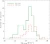Fig. 11 Histograms of 1.4 GHz radio luminosities of our USS sample sources in the B03 (green solid lines) and in the S06 (red dashed lines) fields.

Furthermore, we note that the flux ratio of 1.4 GHz to 3.6 μm (S_{1.4 GHz}/S_{3.6 μm}) versus redshift (z) diagnostic plot suggests that a high cut-off in S_{1.4 GHz}/S_{3.6 μm} can be used to select high-z sources. For example, contamination by low-z star-forming galaxies in our USS sample can be completely removed if we take S_{1.4 GHz}/S_{3.6 μm}> 10. Using S_{1.4 GHz}/S_{3.6 μm} > 10 yields only high-z sources (z ≥ 1) and few radio-strong AGN at lower redshifts. This is consistent with the fact that IFRSs, i.e.,candidate HzRGs, are characterized with a high flux ratio of 1.4 GHz to 3.6 μm (e.g.,S_{1.4 GHz}/S_{3.6 μm} > 50) (Norris et al. 2011a; Collier et al. 2014).

6. Radio luminosities of USS sources

Radio luminosities of USS sources can be used to infer their possible nature, i.e.,radio galaxy, radio-quiet AGN,or star-forming galaxy. We study radio luminosity distributions of our USS sample sources. We use rest-frame radio luminosities that are estimated using k-correction based on spectral index (α) measured between 325 MHz and 1.4 GHz, and assuming the radio emission is synchrotron emission characterized by a power law (S_ν ∝ ν^α). The radio luminosity of a source at redshift z and luminosity-distance d_L is therefore given by ${\mathit{L}}_{\mathit{\nu }}\mathrm{=}\mathrm{4}\mathit{\pi }{\mathit{d}}_{\mathit{L}}^{\mathrm{2}}$S_ν(1 + z)^{−(α + 1)}. Figure 11 shows the 1.4 GHz radio luminosity distributions of our USS sample sources. We note that radio luminosities are available only for USS sources with redshift estimates, i.e.,86/116 sources in the B03 field and 39/44 sources in the S06 field. Table 3 lists the ranges and medians of radio luminosity distributions at 1.4 GHz and 325 MHz of our USS sample sources in the two subfields. Figure 12 shows the 1.4 GHz radio luminosity versus redshift plot. It is clear that most of the low-z (z< 0.5) USS sources have 1.4 GHz radio luminosities (L_{1.4 GHz}) ~10²¹−10²³ W Hz^-1, similar to radio-quiet AGNs and star-forming galaxies, which is consistent with the diagnostics based on the mid-IR colors and the flux ratios of radio to mid-IR. We note that a substantially large fraction (i.e.,55/86 ~ 64% sources in the B03 field, and 31/39 ~ 79.5% sources in the S06 field) of our USS sources do have 1.4 GHz radio luminosity higher than 10²⁴ W Hz^-1. Radio sources with L_{1.4 GHz} > 10²⁴ W Hz^-1 are unlikely to be powered by star formation or starburst galaxies alone (e.g.,Afonso et al. 2005), and are likely to constitute radio sources such as compact steep spectrum (CSS) radio sources, gigahertz peaked spectrum (GPS) radio sources, and FR−I/FR−II radio galaxies. Submillimeter galaxies with obscured AGN at z ~ 2–3, can also have radio luminosities ~10²⁴ W Hz^-1 (Seymour et al. 2009). Powerful USS radio sources (L_{1.4 GHz} > 10²⁴ W Hz^-1) with unresolved radio morphologies can be radio sources with compact sizes and steep spectra, i.e.,CSS and GPS, which are widely thought to represent the start of the evolutionary path to large-scale radio sources (Tinti & de Zotti 2006; Fanti 2009). Most of our USS sample sources remain unresolved in our 325 MHz and 1.4 GHz observations (beamsize ~6.0 arcsec), and therefore high-resolution radio observations are required to determine the morphology, physical extent, and brightness temperature of the radio emitting regions and thus allowing us to probe the AGN nature in obscured environments. In our USS sample, we have a substantial fraction of sources (22/86 ~ 26.6% sources in the B03 field, and 17/39 ~ 43.6% sources in the S06 field) that do have L_{1.4 GHz} ≥ 10²⁵ W Hz^-1, and can be considered as secure candidate radio-loud AGNs (e.g., Jiang et al. 2007; Sajina et al. 2008). Indeed, some of our USS sources (e.g.,GMRT022735-041121, GMRT022743-042130, GMRT022421-042547, GMRT022733-043317, GMRT022728-040344, GMRT021659-044918, GMRT021926-051535, GMRT021827-045440) with L_{1.4 GHz}> 10²⁵ W Hz^-1, clearly show double-lobed radio morphologies at 1.4 GHz, and can be classified as FR−I/FR−II radio galaxies.

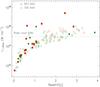Fig. 12 Redshift versus 1.4 GHz luminosity plot for our USS sample sources. Green circles and red squares represent sources in the B03 and the S06 fields, respectively. Filled and open symbols represent sources with the spectroscopic and the photometric redshifts, respectively. The dotted line shows the radio-loud limit (adopted from Jiang et al. 2007; Sajina et al. 2008).

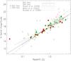Fig. 13 K − z plot for our USS sources. Green circles and red squares represent sources in the B03 and the S06 fields, respectively. Filled and open symbols represent sources with the spectroscopic and the photometric redshifts, respectively. Solid and dashed-triple-dotted lines represent the best fits for sources at redshifts (z) ≥ 0.5 in the B03 and the S06 fields, respectively. The dashed-dotted, dotted and dashed lines represent best fit lines of the K − z relations for the powerful radio galaxy samples from Bryant et al. (2009); Willott et al. (2003); Brookes et al. (2008), respectively. All the magnitudes are in Vega system.

7. The K–z relation for USS sources

It is well known that radio galaxies follow a tight correlation between K-band magnitude and redshift, i.e.,K − z relation (Jarvis et al. 2001b; De Breuck et al. 2002a; Willott et al. 2003; Brookes et al. 2008; Bryant et al. 2009). K-band (centered at 2.2 μm) observations help to study the stellar population in galaxies over a large redshift range (0 ≤ z ≤ 4) as it samples their near-IR to optical rest-frame emission. We investigate the K − z relation for our USS sample sources. The K-band magnitudes in the B03 field and the S06 field are obtained from the VIDEO and the UDS data, respectively. The VIDEO magnitudes are in K_s band however, the difference between K_s and K band magnitudes is small and on the order of typical errors in magnitudes. We used Vega magnitudes, i.e.,VIDEO K-band AB magnitudes were converted to Vega system using the conversion factor (K_AB = K_Vega + 1.9) given in Hewett et al. (2006). Some of the earlier studies (e.g., Eales et al. 1997; Willott et al. 2003; De Breuck et al. 2004) used 8.0 arcsec aperture (i.e.,corresponding to 65 kpc at z = 1) K-band magnitude to account for the variation of K-band emission with aperture size. However, in a sample that consists of radio sources with a wide range of flux densities and redshifts, a 4.0 arcsec diameter aperture adequately samples nearly the entire K-band emission and reduces the photometric uncertainty (Bryant et al. 2009; Simpson et al. 2012). Therefore, we use 4.0 arcsec diameter aperture K-band magnitude at all redshifts. To find and remove quasars, we performed cross-matching of our USS sample with the SDSS⁹ DR10 quasar catalog using search radius of 3.0 arcsec. However, we do not find a counterpart of any USS source in the SDSS quasar catalog. Therefore, we include all our USS sources in the K − z plot.

Figure 13 shows the K − z plot for our USS sources with K-band magnitudes ranging from 12.0 Mag to 23.0 Mag, and redshifts spanning over 0.03 to 3.8. It is evident that the K − z relation continues to hold for our faint USS sources, although with larger scatter compared to the powerful radio galaxies. We find that the best linear fits for the USS sources in the B03 and the S06 fields can be represented as K = 17.89 + 1.99log (z), and K = 18.36 + 2.48log (z), respectively, with correlation coefficients 0.73 and 0.61, respectively. The best fits and correlation coefficients are obtained by using only sources with redshift (z) ≥ 0.5 as the low-z USS sources are likely to be contaminated by non-AGN star-forming galaxies which exhibit larger scatter. The comparison of the K − z relation for our USS sample sources with that for powerful radio galaxies, i.e.,samples from Willott et al. (2003), Brookes et al. (2008), and Bryant et al. (2009), shows that the K − z relation for our faint USS sources is consistent with the one seen for bright powerful radio galaxies, however, with a larger scatter. The deeper K-band UDS data in the S06 field results in the detection of faint sources at higher redshifts (z ≥ 1.0). These sources tend to deviate from the K − z relation observed for powerful radio galaxies. We note that only photometric redshift estimates are available for these sources. Generally, sources with photometric redshifts tend to show larger scatter than the ones with spectroscopic redshifts and therefore, inaccurate photometric redshift estimates may be partly responsible for the larger scatter. The contamination by AGNs of low radio luminosity can attribute to larger scatter (e.g., De Breuck et al. 2002a; Simpson et al. 2012). Faint radio sources are known to exhibit systematically fainter K-band magnitudes than bright radio sources at a given redshift (e.g., Eales et al. 1997; Willott et al. 2003), which is attributed to different stellar luminosities of their host galaxies. Furthermore, in our USS sample, we have a significant fraction (~26% in the B03 field and ~8% in the S06 field) of sources that remained unidentified in the K-band, and these can be considered as potential high-z candidates.

8. High-z radio sources in faint USS sample

In our study we use the USS technique to select high-z sources. The efficiency of the USS technique in selecting high-z sources is based on the existence of the correlation between redshift and radio spectral index, i.e.,z-α correlation (Klamer et al. 2006; Ker et al. 2012). It has been shown that USS samples display higher median redshifts than that for full radio samples (e.g., Bryant et al. 2009). The USS samples selected at different flux limits have achieved varying degrees of success in selecting high-z sources. There are suggestions that the USS method is more efficient in selecting high-z sources at the flux density limit of approximately 10 mJy at 1.4 GHz, while the fraction of high-z sources decreases at lower and higher flux densities (e.g., Dunlop & Peacock 1990; Best et al. 2003). In the literature, many studies of the USS samples have also used additional selection criteria such as small angular size and faint infrared magnitude to select high-z sources (De Breuck et al. 2004, 2006; Cruz et al. 2006). According to the K − z relation, HzRGs are expected to be faint in K-band and indeed, several HzRGs have been discovered by pre-selecting them in K-band (Jarvis et al. 2001b; Brookes et al. 2006; Jarvis et al. 2009). The second highest redshift known radio galaxy identified by Jarvis et al. (2009) was selected for follow-up based purely on its faint K-band magnitude, and it is not a USS source (α = − 0.75). As discussed in Sect. 5.2, the radio sources without optical or infrared detections, i.e.,IFRS also potentially sample high-z sources (Norris et al. 2011a; Middelberg et al. 2011). Thus, the K-band/IR magnitude based methods are alternative efficient techniques for selecting high-z sources, and can be feasible over large sky areas with the availability of deep IR and radio surveys. A detailed discussion on the comparison of the efficiencies of the USS method and K-band/IR based methods to select high-z sources is beyond the scope of this paper.

In order to asses how efficient our faint USS sample is in selecting high-z sources, we compare the median redshifts and the fraction of faint K-band USS sources in our USS sample to that for well known bright USS samples. In Table 4, we present a comparison of various parameters, i.e.,flux limits, USS source densities, median redshifts and the fraction of faint K-band sources in our faint USS sample to these same parameters in bright USS samples. We find that the USS source density in our sample is nearly 1000 times higher than that for the bright samples, e.g.,6C^⋆ (Jarvis et al. 2001b), SUMSS-NVSS (De Breuck et al. 2004), WENSS-NVSS (De Breuck et al. 2000, 2002a). This can understood as we are probing at sub-mJy regime which is two order of magnitude deeper than the bright USS sample flux limits, i.e.,10–15 mJy in shallow and wide area surveys. The comparison of median redshifts shows that our faint USS sample has median redshift similar to the one for the SUMSS-NVSS sample, although, the 6C^⋆, WENSS-NVSS samples do have higher median redshifts. It is to be noted that the bright samples have additional biases due to K-band selection and incomplete spectroscopic redshifts, and hence a direct comparison may not be viable, but it is interesting to note that the median redshifts are broadly consistent. In Table 4, we also present the comparison of the fraction of USS sources with K-band magnitude fainter than 19.5 Vega magnitude (K> 19.5). The fraction of faint K-band sources in the sample can be used as an indicator of the fraction of high-z sources owing to the K − z relation. We note that the fraction of USS sources with K > 19.5 in our sample is ~30%, similar to that found in the bright USS samples, e.g.,WENSS-NVSS, TEXAS-NVSS, and SUMSS-NVSS. Moreover, K-band photometry of the WENSS-NVSS sample is not complete as most of the sources observed in K-band were pre-selected to be those which were not detected in optical imaging. This kind of pre-selection is likely to remove a significant fraction of intermediate redshift sources with K< 19.5.

In conclusion, we state that the comparison of the median redshifts and the fractions of USS sources with faint K-band magnitudes of our sample with that of the bright USS samples, suggests that even at faint flux density, the USS selection is an efficient method to select high-z sources. The high-z USS sources in our sample do have faint optical/IR counterparts (see Sects. 3 and 5) and this may be the combined effect of the z − α correlation and the K − z correlation. Our study on the faint USS sources limited to small sky area (i.e.,1.8 deg^-2) can be used as the basis to search for high-z sources via USS technique in the next generation wide and deep radio continuum surveys down to the μJy level e.g.,from SKA pathfinders (Norris et al. 2011b, 2013) and LOFAR (van Haarlem et al. 2013). The deep optical/IR follow up surveys, e.g.,from LSST (Ivezic et al. 2008), JWST (Gardner et al. 2006), WFIRST (Green et al. 2012), will help us in obtaining photometric redshifts and in removing low redshift contaminants.

9. Conclusions

Using the most sensitive 325 MHz GMRT observations (5σ ~ 800 μJy) and 1.4 GHz VLA observations (5σ ~ 80–100 μJy) available for two subfields in the XMM-LSS field, we derive a large sample of 160 faint USS sources (${\mathit{\alpha }}_{\mathrm{325}\mathrm{MHz}}^{\mathrm{1.4}\mathrm{GHz}}\mathrm{\le }\mathrm{-}\mathrm{1}$). Our study is one of the few attempts made in the literature to characterize the population of faint USS sources down to the sub-mJy level, and to search for HzRG candidates. The availability of deep optical, near-IR, and mid-IR data in the two subfields allow us to identify counterparts of the majority of our USS sample sources, and to unveil their nature. The conclusions of our study are:

• 1.

  Using the CFHTLS-D1 optical data (${\mathit{r}}_{\mathrm{AB}}^{\mathrm{\prime }}\mathrm{~}\mathrm{26}$.1) in theB03 field, and Subaru/SuprimeCamdata (R_AB ~ 27.7) in the S06 field, we find optical counterparts of86/116 ~ 74% and 37/39[en-tity!#x2009!]~ 95% USS sources in thetwo subfields, respectively. In near-IR, the VIDEO data(K_AB ~ 23.5), and the UDS data (K_AB ~ 24.6) yield similar high identificationrates, i.e.,86/116 ~ 74%and 35/38 ~ 92% in theB03 and the S06 fields, respectively. The Spitzer surveysat 3.6 μm and 4.5 μm, i.e.,theSERVS data ([3.6]_AB ~ 23.1) in the B03 field, andSpUDS data ([3.6]_AB ~ 24.0) in the S06 field yield counterparts for72/95 ~ 76% and 32/36[en-tity!#x2009!]~ 89% USS sources in the twosubfields, respectively (see Table 2). We findthat, compared to full radio population, the optical and IR magni-tude distributions of USS sources are systematically flatter andfainter. This can be interpreted as the possible dusty and/or high-znature of USS sources.

• 2.

  Redshift estimates are available for 86/116 ~ 74% and 39/44 ~ 89% of the USS sources in the B03 and the S06 field, respectively. The distributions of available redshifts for our USS sample sources span from z ~ 0.03 to 3.86 with the median values z_median ~ 1.18, and z_median ~ 1.57 in the B03 and the S06 fields, respectively. The lower median redshift in the B03 field can be attributed to the fact that the redshift estimates are not available for a large fraction (30/116 ~ 26%) of USS sources, and the radio to mid-IR flux ratio diagnostic suggests these to be potentially high redshift candidates. The USS sources show higher median redshifts than the non-USS radio sources. The comparison of the redshift distributions of our USS sources with the one for the radio population derived by using the SKADS Simulated Skies (S³) simulations, shows that our faint USS sample efficiently selects high-z sources. However, because of the faint flux density limit our USS sample may be dominated by the less powerful radio-loud sources.

• 3.

  The mid-IR color–color diagnostics are consistent with most of our USS sample sources at higher redshifts (z> 0.5) being mainly AGN. However, at low redshift (z< 0.5) the USS sample may contain sources in which mid-IR colors are dominated by the emission due to star formation.

• 4.

  A substantially large fraction of our USS sources (nearly 33/88 ~ 38% in the B03 field and 21/36 ~ 58% in the S06 field) have radio to mid-IR flux ratios (S_{1.4 GHz}/S_{3.6 μm}) from ~4 to 100, distributed over z ~ 0.5 to 3.8. The locations of these USS sources in the radio to mid-IR flux ratio (S_{1.4 GHz}/S_{3.6 μm}) versus redshift diagnostic plot is similar to those observed for submillimeter galaxies in the representative sample of Norris et al. (2011). The radio luminosities (L_{1.4 GHz} ≥ 10²⁴ W Hz^-1) and compact radio sizes suggest these USS sources to be potentially weakly radio-loud AGN hosted in obscured environments.

• 5.

  There are 23/88 ~ 26% USS source in the B03 field, and 4/36 ~ 11% USS source in the S06 field that do not have 3.6 μm detection and exhibit high radio to mid-IR flux ratio limits, i.e.,S_{1.4 GHz}/S_{3.6 μm} > 50. The flux ratios of these USS sources are similar to the ones observed for radio-loud AGNs and powerful HzRGs, and therefore, these USS sources can be considered as HzRGs candidates.

• 6.

  Radio luminosity distributions of our USS sources span over a wide range e.g.,L_{1.4 GHz} ~ 10²¹ − 10²⁷ W Hz^-1. A significant fraction of our USS sources (i.e.,22/86 ~ 26.6% sources in the B03 field, and 17/39 ~ 43.6% sources in the S06 field), do have L_{1.4 GHz} ≥ 10²⁵ W Hz^-1, and can be considered as secure candidate radio-loud AGNs. USS sources of high radio luminosities (L_{1.4 GHz}> 10²⁴ W Hz^-1) with unresolved radio morphologies can be sources with compact sizes and steep spectra e.g.,CSS and GPS, which are thought to represent the start of the evolutionary path to large-scale radio sources (Tinti & de Zotti 2006; Fanti 2009). However, high-resolution radio observations are required to determine the morphology, physical extent, and brightness temperature of the radio emitting regions and probe their nature.

• 7.

  Our USS sources follow the K − z relation, although with larger scatter compared to powerful radio galaxies. The comparison of the K − z relation of our USS sources with that of HzRGs suggests that apart from HzRG candidates our USS sample also contains radio sources of various classes such as weakly radio-loud sources at higher redshifts and radio-quiet AGNs at low redshift.

• 8.

  Our study demonstrates that the criterion of ultra steep spectral index remains an efficient method to select high redshift sources even at sub-mJy flux densities. We find that, in addition to powerful HzRG candidates, faint USS sample also contain weak radio-loud AGNs likely to be hosted in obscured environments. In our forthcoming paper we shall investigate the nature of obscured environments of these sources using far-IR/submm observations from Herschel.

Online material

Appendix A: Our USS sample

In Table A.1 we list all our USS sample sources derived from 325 MHz and 1.4 GHz observations.

Acknowledgments

We gratefully acknowledge generous support from the Indo-French Center for the Promotion of Advanced Research (Centre Franco-Indien pour la Promotion de la Recherche Avancée) under program No. 4404-3. We thank the staff of GMRT who have made these observations possible. GMRT is run by the National Centre for Radio Astrophysics of the Tata Institute of Fundamental Research. We thank Marco Bondi for providing 1.4 GHz and 610 MHz radio images of VVDS field. We thank Chris Simpson for providing 1.4 GHz VLA radio image of SXDF field. We also thank the anonymous referee for useful comments which helped to improve the manuscript. This work is based on observations made with the Spitzer Space Telescope, which is operated by the Jet Propulsion Laboratory (JPL), California Institute of Technology (Caltech), under a contract with NASA. This work used the CFHTLS data products, which are based on observations obtained with MegaPrime/MegaCam, a joint project of CFHT and CEA/DAPNIA, at the CFHT which is operated by the National Research Council (NRC) of Canada, the Institut National des Sciences de l’Univers of the Centre National de la Recherche Scientifique (CNRS) of France, and the University of Hawaii. This work is based in part on data products produced at TERAPIX and the Canadian Astronomy Data Centre as part of the CFHTLS, a collaborative project of NRC and CNRS. This research uses data from the VIMOS VLT Deep Survey, obtained from the VVDS database operated by Cesam, Laboratoire d’Astrophysique de Marseille, France.

References

All Tables

All Figures

	Fig. 1 Footprints of VLA-VVDS (B03 field; in blue), SXDF (S06 field; in brown), VIDEO (in green), SERVS (in magenta), UDS (in cyan), SpUDS (in red), and SWIRE (in yellow) fields overplotted on our 325 MHz GMRT image. CFHTLS-D1 covers the same area as VLA-VVDS.
In the text

Fig. 2 Histogram of 325 MHz to 1.4 GHz spectral index (${\mathit{\alpha }}_{\mathrm{325}\mathrm{MHz}}^{\mathrm{1.4}\mathrm{GHz}}$). Green solid line histogram represents sources in the B03 field while red dashed line histogram represents sources in the S06 field. Median spectral indices in the B03 field (${\mathit{\alpha }}_{\mathrm{325}\mathrm{MHz}\mathit{,}\mathrm{median}}^{\mathrm{1.4}\mathrm{GHz}}\mathrm{~}\mathrm{-}\mathrm{0.87}$) and in the S06 field (${\mathit{\alpha }}_{\mathrm{325}\mathrm{MHz}\mathit{,}\mathrm{median}}^{\mathrm{1.4}\mathrm{GHz}}\mathrm{~}\mathrm{-}\mathrm{0.76}$) are represented by vertical green dashed-dotted and red dashed lines, respectively. USS limit (${\mathit{\alpha }}_{\mathrm{325}\mathrm{MHz}}^{\mathrm{1.4}\mathrm{GHz}}\mathrm{\le }\mathrm{-}\mathrm{1}$) is represented by the vertical dotted line.

In the text

Fig. 3 Spectral index (${\mathit{\alpha }}_{\mathrm{325}\mathrm{MHz}}^{\mathrm{1.4}\mathrm{GHz}}$) versus 1.4 GHz flux density plot. Plus (+) and cross (×) symbols represent USS sources in the B03 and in the S06 fields, respectively. The dashed line represents the median spectral index value (${\mathit{\alpha }}_{\mathrm{325}\mathrm{MHz}}^{\mathrm{1.4}\mathrm{GHz}}\mathrm{~}\mathrm{-}\mathrm{0.83}$) for the full sample. The flux density limits at 325 MHz and 1.4 GHz are represented by dotted and long-dashed lines, respectively.

In the text

Fig. 4 Histograms of R-band magnitudes of the USS sources and of the full 1.4 GHz radio population in the B03 and the S06 field. Histograms of USS sources are shown by green solid lines and red long dashed lines for the B03 and the S06 fields, respectively. While green dashed and red dashed-dotted lines represent histograms for the full 1.4 GHz radio population in the B03 and the S06 fields, respectively.

In the text

Fig. 5 Histograms of K-band magnitudes of the USS sources and of the full 1.4 GHz radio population in the B03 and the S06 field. Histograms of USS sources are shown by green solid lines and red long dashed lines for the B03 and the S06 fields, respectively. Green dashed and red dashed-dotted lines represent histograms for the full 1.4 GHz radio population in the B03 and the S06 fields, respectively.

In the text

	Fig. 6 Histograms of 3.6 μm magnitudes of the USS sources and of the full 1.4 GHz radio population in the B03 and S06 field. Histograms of USS sources are shown by green solid lines and red long dashed lines for the B03 and the S06 fields, respectively. Green dashed and red dashed-dotted lines represent histograms for full 1.4 GHz radio population in the B03 and the S06 fields, respectively.
In the text

	Fig. 7 Comparison between the spectroscopic and the photometric redshifts of the USS sources in the B03 field (green circles) and in the S03 field (red squares). The diagonal line represents zspec = zphot.
In the text

Fig. 8 Redshift distributions of our USS sources in the B03 field (in green solid lines) and in the S06 field (in red dashed lines). Redshift estimates are available for 86/116 and 39/44 USS sources in the B03 field and the S06 field, respectively. The redshift distributions of 1.4 GHz radio population predicted by SKA simulated skies (SKADS; Wilman et al. 2008, 2010) for the B03 and the S06 fields are plotted with dotted and dashed curves, respectively. The flux limit S1.4 GHz ~ 100 μJy and sky area of 1.0 deg-2 in the B03 field and 0.8 deg-2 in the S06 field are used to obtain simulated radio populations for the two subfields, respectively. The redshift distributions of simulated radio populations in the B03 and the S06 fields are presented in McAlpine et al. (2013) and Simpson et al. (2012), respectively. The uneven variations seen in the SKADS simulated redshift distribution in the B03 field can be attributed to the clustering of radio sources manifested as cosmic variance in this relatively small field.

In the text

Fig. 9 Mid-IR color–color diagnostic plots for our USS sources in both the B03 and S06 fields. Left and right panels show mid-IR color–color plots based on Lacy et al. (2004) and Stern et al. (2005) criteria, respectively. Filled and open symbols represent USS sources and 1.4 GHz radio populations, respectively. USS sources of different redshifts are shown with different colors. The regions bounded by dashed lines denotes AGN selection wedge. Lacy et al. (2004) defined the AGN selection wedge as: (log(S5.8/S3.6) > −0.1) ∧ (log(S8.0/S4.5) > −0.8) ∧ (log(S8.0/S4.5) ≤ 0.8 log(S5.8/S3.6) + 0.5); where ∧ is “AND” operator. While, the AGN selection wedge proposed by Stern et al. (2005) is defined as: ([5.8] – [8.0] > 0.6) ∧ ([3.6] – [4.5] > 0.2([5.8] – [8.0]) + 0.18) ∧ ([3.6] – [4.5 ] > 2.5 ([5.8]–[8.0]) – 3.5); where IRAC magnitudes are in the Vega system. We converted IRAC AB magnitudes to Vega magnitudes (mAB = mVega + conv) using conversion factors 2.78, 3.26, 3.75, and 4.38 for 3.6 μm, 4.5 μm, 5.8 μm, and 8.0 μm bands, respectively (see IRAC Data HandBook 3.0 2006).

In the text

Fig. 10 Ratio of 1.4 GHz radio flux density to 3.6 μm flux (S1.4 GHz/S3.6 μm) versus redshift plot for our USS sources. USS sources of different radio luminosities are represented with different colors. USS sources without redshift estimates are shown at the rightmost position. USS sources with only lower limits on the flux ratios (S1.4 GHz/S3.6 μm), i.e.,without 3.6 μm detections, are shown by upward arrows. The area above the dotted line represents the range of flux ratios for the powerful HzRGs and IFRSs. Tracks indicating the regions for the different classes of sources are taken from Norris et al. (2011a). The solid lines represent the loci of LIRGs and ULIRGs using Rieke et al. (2009) SED templates. The dashed (long dashed) line indicates the loci of radio-loud (radio-quiet) QSOs from Elvis et al. (1994). We caution that dust extinction can cause any of these tracks to rise steeply at high redshift where the observed 3.6 μm is emitted in visible wavelengths at the rest frame.

In the text

	Fig. 11 Histograms of 1.4 GHz radio luminosities of our USS sample sources in the B03 (green solid lines) and in the S06 (red dashed lines) fields.
In the text

	Fig. 12 Redshift versus 1.4 GHz luminosity plot for our USS sample sources. Green circles and red squares represent sources in the B03 and the S06 fields, respectively. Filled and open symbols represent sources with the spectroscopic and the photometric redshifts, respectively. The dotted line shows the radio-loud limit (adopted from Jiang et al. 2007; Sajina et al. 2008).
In the text

Fig. 13 K − z plot for our USS sources. Green circles and red squares represent sources in the B03 and the S06 fields, respectively. Filled and open symbols represent sources with the spectroscopic and the photometric redshifts, respectively. Solid and dashed-triple-dotted lines represent the best fits for sources at redshifts (z) ≥ 0.5 in the B03 and the S06 fields, respectively. The dashed-dotted, dotted and dashed lines represent best fit lines of the K − z relations for the powerful radio galaxy samples from Bryant et al. (2009); Willott et al. (2003); Brookes et al. (2008), respectively. All the magnitudes are in Vega system.

In the text

References

- Adami, C., Mazure, A., Pierre, M., et al. 2011, A&A, 526, A18 [NASA ADS] [CrossRef] [EDP Sciences] [Google Scholar]
- Afonso, J., Georgakakis, A., Almeida, C., et al. 2005, ApJ, 624, 135 [NASA ADS] [CrossRef] [Google Scholar]
- Afonso, J., Bizzocchi, L., Ibar, E., et al. 2011, ApJ, 743, 122 [NASA ADS] [CrossRef] [Google Scholar]
- Alonso-Herrero, A., Pérez-González, P. G., Alexander, D. M., et al. 2006, ApJ, 640, 167 [NASA ADS] [CrossRef] [Google Scholar]
- Banerji, M., Chapman, S. C., Smail, I., et al. 2011, MNRAS, 418, 1071 [NASA ADS] [CrossRef] [Google Scholar]
- Bardelli, S., Zucca, E., Bolzonella, M., et al. 2009, A&A, 495, 431 [NASA ADS] [CrossRef] [EDP Sciences] [Google Scholar]
- Barmby, P., Huang, J.-S., Ashby, M. L. N., et al. 2008, ApJS, 177, 431 [NASA ADS] [CrossRef] [Google Scholar]
- Basu, A., Mitra, D., Wadadekar, Y., & Ishwara-Chandra, C. H. 2012, MNRAS, 419, 1136 [NASA ADS] [CrossRef] [Google Scholar]
- Best, P. N., Longair, M. S., & Roettgering, H. J. A. 1998, MNRAS, 295, 549 [NASA ADS] [CrossRef] [Google Scholar]
- Best, P. N., Arts, J. N., Röttgering, H. J. A., et al. 2003, MNRAS, 346, 627 [NASA ADS] [CrossRef] [Google Scholar]
- Blundell, K. M., Rawlings, S., Eales, S. A., Taylor, G. B., & Bradley, A. D. 1998, MNRAS, 295, 265 [NASA ADS] [CrossRef] [Google Scholar]
- Blundell, K. M., Rawlings, S., & Willott, C. J. 1999, AJ, 117, 677 [Google Scholar]
- Bondi, M., Ciliegi, P., Zamorani, G., et al. 2003, A&A, 403, 857 [NASA ADS] [CrossRef] [EDP Sciences] [Google Scholar]
- Bondi, M., Ciliegi, P., Venturi, T., et al. 2007, A&A, 463, 519 [NASA ADS] [CrossRef] [EDP Sciences] [Google Scholar]
- Bornancini, C. G., De Breuck, C., de Vries, W., et al. 2007, MNRAS, 378, 551 [NASA ADS] [CrossRef] [Google Scholar]
- Bornancini, C. G., O’Mill, A. L., Gurovich, S., & Lambas, D. G. 2010, MNRAS, 406, 197 [NASA ADS] [CrossRef] [Google Scholar]
- Brammer, G. B., van Dokkum, P. G., & Coppi, P. 2008, ApJ, 686, 1503 [NASA ADS] [CrossRef] [Google Scholar]
- Broderick, J. W., Bryant, J. J., Hunstead, R. W., Sadler, E. M., & Murphy, T. 2007, MNRAS, 381, 341 [NASA ADS] [CrossRef] [Google Scholar]
- Brookes, M. H., Best, P. N., Rengelink, R., & Röttgering, H. J. A. 2006, MNRAS, 366, 1265 [NASA ADS] [CrossRef] [Google Scholar]
- Brookes, M. H., Best, P. N., Peacock, J. A., Röttgering, H. J. A., & Dunlop, J. S. 2008, MNRAS, 385, 1297 [NASA ADS] [CrossRef] [Google Scholar]
- Bryant, J. J., Johnston, H. M., Broderick, J. W., et al. 2009, MNRAS, 395, 1099 [NASA ADS] [CrossRef] [Google Scholar]
- Chambers, K. C., Miley, G. K., van Breugel, W. J. M., et al. 1996, ApJS, 106, 247 [NASA ADS] [CrossRef] [Google Scholar]
- Chuter, R. W., Almaini, O., Hartley, W. G., et al. 2011, MNRAS, 413, 1678 [NASA ADS] [CrossRef] [Google Scholar]
- Ciliegi, P., Zamorani, G., Bondi, M., et al. 2005, A&A, 441, 879 [NASA ADS] [CrossRef] [EDP Sciences] [Google Scholar]
- Cohen, A. S., Röttgering, H. J. A., Kassim, N. E., et al. 2003, ApJ, 591, 640 [NASA ADS] [CrossRef] [Google Scholar]
- Cohen, A. S., Röttgering, H. J. A., Jarvis, M. J., Kassim, N. E., & Lazio, T. J. W. 2004, ApJS, 150, 417 [NASA ADS] [CrossRef] [Google Scholar]
- Collier, J. D., Banfield, J. K., Norris, R. P., et al. 2014, MNRAS, 439, 545 [NASA ADS] [CrossRef] [Google Scholar]
- Condon, J. J., Cotton, W. D., Greisen, E. W., et al. 1998, AJ, 115, 1693 [NASA ADS] [CrossRef] [Google Scholar]
- Croton, D. J., Springel, V., White, S. D. M., et al. 2006, MNRAS, 365, 11 [NASA ADS] [CrossRef] [Google Scholar]
- Cruz, M. J., Jarvis, M. J., Blundell, K. M., et al. 2006, MNRAS, 373, 1531 [NASA ADS] [CrossRef] [Google Scholar]
- De Breuck, C., Brotherton, M. S., Tran, H. D., van Breugel, W., & Röttgering, H. J. A. 1998, AJ, 116, 13 [Google Scholar]
- De Breuck, C., van Breugel, W., Röttgering, H. J. A., & Miley, G. 2000, A&AS, 143, 303 [NASA ADS] [CrossRef] [EDP Sciences] [Google Scholar]
- De Breuck, C., Tang, Y., de Bruyn, A. G., Röttgering, H., & van Breugel, W. 2002a, A&A, 394, 59 [NASA ADS] [CrossRef] [EDP Sciences] [Google Scholar]
- De Breuck, C., van Breugel, W., Stanford, S. A., et al. 2002b, AJ, 123, 637 [NASA ADS] [CrossRef] [Google Scholar]
- De Breuck, C., Hunstead, R. W., Sadler, E. M., Rocca-Volmerange, B., & Klamer, I. 2004, MNRAS, 347, 837 [NASA ADS] [CrossRef] [Google Scholar]
- De Breuck, C., Downes, D., Neri, R., et al. 2005, A&A, 430, L1 [NASA ADS] [CrossRef] [EDP Sciences] [Google Scholar]
- De Breuck, C., Klamer, I., Johnston, H., et al. 2006, MNRAS, 366, 58 [NASA ADS] [CrossRef] [Google Scholar]
- Donley, J. L., Rieke, G. H., Rigby, J. R., & Pérez-González, P. G. 2005, ApJ, 634, 169 [NASA ADS] [CrossRef] [Google Scholar]
- Donley, J. L., Rieke, G. H., Pérez-González, P. G., Rigby, J. R., & Alonso-Herrero, A. 2007, ApJ, 660, 167 [NASA ADS] [CrossRef] [Google Scholar]
- Donley, J. L., Rieke, G. H., Pérez-González, P. G., & Barro, G. 2008, ApJ, 687, 111 [NASA ADS] [CrossRef] [Google Scholar]
- Donley, J. L., Koekemoer, A. M., Brusa, M., et al. 2012, ApJ, 748, 142 [NASA ADS] [CrossRef] [Google Scholar]
- Dunlop, J. S., & Peacock, J. A. 1990, MNRAS, 247, 19 [NASA ADS] [Google Scholar]
- Dunlop, J., Akiyama, M., Alexander, D., et al. 2007, Spitzer Proposal, 40021 [Google Scholar]
- Eales, S., Rawlings, S., Law-Green, D., Cotter, G., & Lacy, M. 1997, MNRAS, 291, 593 [NASA ADS] [CrossRef] [Google Scholar]
- Eales, S. A., & Rawlings, S. 1996, ApJ, 460, 68 [NASA ADS] [CrossRef] [Google Scholar]
- Elvis, M., Wilkes, B. J., McDowell, J. C., et al. 1994, ApJS, 95, 1 [NASA ADS] [CrossRef] [Google Scholar]
- Fanti, C. 2009, Astron. Nachr., 330, 120 [NASA ADS] [CrossRef] [Google Scholar]
- Fiolet, N., Omont, A., Polletta, M., et al. 2009, A&A, 508, 117 [NASA ADS] [CrossRef] [EDP Sciences] [Google Scholar]
- Galametz, A., Stern, D., De Breuck, C., et al. 2012, ApJ, 749, 169 [NASA ADS] [CrossRef] [Google Scholar]
- Gardner, J. P., Mather, J. C., Clampin, M., et al. 2006, Space Sci. Rev., 123, 485 [NASA ADS] [CrossRef] [Google Scholar]
- Geach, J. E., Simpson, C., Rawlings, S., Read, A. M., & Watson, M. 2007, MNRAS, 381, 1369 [NASA ADS] [CrossRef] [Google Scholar]
- Green, J., Schechter, P., Baltay, C., et al. 2012 [arXiv:1208.4012] [Google Scholar]
- Griffith, R. L., & Stern, D. 2010, AJ, 140, 533 [Google Scholar]
- Gürkan, G., Hardcastle, M. J., & Jarvis, M. J. 2014, MNRAS, 438, 1149 [NASA ADS] [CrossRef] [Google Scholar]
- Hardcastle, M. J., Evans, D. A., & Croston, J. H. 2007, MNRAS, 376, 1849 [NASA ADS] [CrossRef] [Google Scholar]
- Heesen, V., Beck, R., Krause, M., & Dettmar, R.-J. 2009, A&A, 494, 563 [NASA ADS] [CrossRef] [EDP Sciences] [Google Scholar]
- Hewett, P. C., Warren, S. J., Leggett, S. K., & Hodgkin, S. T. 2006, MNRAS, 367, 454 [NASA ADS] [CrossRef] [Google Scholar]
- Huynh, M. T., Norris, R. P., Siana, B., & Middelberg, E. 2010, ApJ, 710, 698 [NASA ADS] [CrossRef] [Google Scholar]
- Ibar, E., Ivison, R. J., Biggs, A. D., et al. 2009, MNRAS, 397, 281 [NASA ADS] [CrossRef] [Google Scholar]
- Ibar, E., Ivison, R. J., Best, P. N., et al. 2010, MNRAS, 401, L53 [NASA ADS] [CrossRef] [Google Scholar]
- Ilbert, O., Arnouts, S., McCracken, H. J., et al. 2006, A&A, 457, 841 [NASA ADS] [CrossRef] [EDP Sciences] [Google Scholar]
- Intema, H. T., van Weeren, R. J., Röttgering, H. J. A., & Lal, D. V. 2011, A&A, 535, A38 [NASA ADS] [CrossRef] [EDP Sciences] [Google Scholar]
- Ishwara-Chandra, C. H., Sirothia, S. K., Wadadekar, Y., Pal, S., & Windhorst, R. 2010, MNRAS, 405, 436 [NASA ADS] [Google Scholar]
- Ivezic, Z., Tyson, J. A., Acosta, E., et al. 2008 [arXiv:0805.2366] [Google Scholar]
- Jarvis, M. J., Rawlings, S., Lacy, M., et al. 2001a, MNRAS, 326, 1563 [NASA ADS] [CrossRef] [Google Scholar]
- Jarvis, M. J., Rawlings, S., Willott, C. J., et al. 2001b, MNRAS, 327, 907 [NASA ADS] [CrossRef] [Google Scholar]
- Jarvis, M. J., Cruz, M. J., Cohen, A. S., Röttgering, H. J. A., & Kassim, N. E. 2004, MNRAS, 355, 20 [NASA ADS] [CrossRef] [Google Scholar]
- Jarvis, M. J., Teimourian, H., Simpson, C., et al. 2009, MNRAS, 398, L83 [NASA ADS] [CrossRef] [Google Scholar]
- Jarvis, M. J., Bonfield, D. G., Bruce, V. A., et al. 2013, MNRAS, 428, 1281 [NASA ADS] [CrossRef] [Google Scholar]
- Jiang, L., Fan, X., Ivezić, Ž., et al. 2007, ApJ, 656, 680 [NASA ADS] [CrossRef] [Google Scholar]
- Ker, L. M., Best, P. N., Rigby, E. E., Röttgering, H. J. A., & Gendre, M. A. 2012, MNRAS, 420, 2644 [NASA ADS] [CrossRef] [Google Scholar]
- Klamer, I. J., Ekers, R. D., Sadler, E. M., et al. 2005, ApJ, 621, L1 [NASA ADS] [CrossRef] [Google Scholar]
- Klamer, I. J., Ekers, R. D., Bryant, J. J., et al. 2006, MNRAS, 371, 852 [NASA ADS] [CrossRef] [Google Scholar]
- Kodama, T., Tanaka, I., Kajisawa, M., et al. 2007, MNRAS, 377, 1717 [NASA ADS] [CrossRef] [Google Scholar]
- Krolik, J. H., & Chen, W. 1991, AJ, 102, 1659 [NASA ADS] [CrossRef] [Google Scholar]
- Lacy, M., Storrie-Lombardi, L. J., Sajina, A., et al. 2004, ApJS, 154, 166 [NASA ADS] [CrossRef] [Google Scholar]
- Lawrence, A., Warren, S. J., Almaini, O., et al. 2007, MNRAS, 379, 1599 [NASA ADS] [CrossRef] [MathSciNet] [Google Scholar]
- Lee, J. C., Hwang, H. S., Lee, M. G., Kim, M., & Lee, J. H. 2012, ApJ, 756, 95 [NASA ADS] [CrossRef] [Google Scholar]
- Le Fèvre, O., Vettolani, G., Garilli, B., et al. 2005, A&A, 439, 845 [NASA ADS] [CrossRef] [EDP Sciences] [Google Scholar]
- Le Fèvre, O., Cassata, P., Cucciati, O., et al. 2013, A&A, 559, A14 [NASA ADS] [CrossRef] [EDP Sciences] [Google Scholar]
- Leroy, A. K., Evans, A. S., Momjian, E., et al. 2011, ApJ, 739, L25 [NASA ADS] [CrossRef] [Google Scholar]
- Mangalam, A. V., & Gopal-Krishna. 1995, MNRAS, 275, 976 [NASA ADS] [CrossRef] [Google Scholar]
- Martínez-Sansigre, A., Rawlings, S., Lacy, M., et al. 2005, Nature, 436, 666 [NASA ADS] [CrossRef] [Google Scholar]
- Martínez-Sansigre, A., Karim, A., Schinnerer, E., et al. 2009, ApJ, 706, 184 [NASA ADS] [CrossRef] [Google Scholar]
- Mauduit, J.-C., Lacy, M., Farrah, D., et al. 2012, PASP, 124, 714 [NASA ADS] [CrossRef] [Google Scholar]
- McAlpine, K., Jarvis, M. J., & Bonfield, D. G. 2013, MNRAS, 436, 1084 [NASA ADS] [CrossRef] [Google Scholar]
- McLure, R. J., Willott, C. J., Jarvis, M. J., et al. 2004, MNRAS, 351, 347 [NASA ADS] [CrossRef] [Google Scholar]
- Middelberg, E., Norris, R. P., Tingay, S., et al. 2008, A&A, 491, 435 [NASA ADS] [CrossRef] [EDP Sciences] [Google Scholar]
- Middelberg, E., Norris, R. P., Hales, C. A., et al. 2011, A&A, 526, A8 [NASA ADS] [CrossRef] [EDP Sciences] [Google Scholar]
- Miley, G., & De Breuck, C. 2008, A&ARv, 15, 67 [NASA ADS] [CrossRef] [Google Scholar]
- Norris, R. P., Tingay, S., Phillips, C., et al. 2007, MNRAS, 378, 1434 [NASA ADS] [CrossRef] [Google Scholar]
- Norris, R. P., Afonso, J., Cava, A., et al. 2011a, ApJ, 736, 55 [NASA ADS] [CrossRef] [Google Scholar]
- Norris, R. P., Hopkins, A. M., Afonso, J., et al. 2011b, PASA, 28, 215 [NASA ADS] [CrossRef] [Google Scholar]
- Norris, R. P., Lenc, E., Roy, A. L., & Spoon, H. 2012, MNRAS, 422, 1453 [NASA ADS] [CrossRef] [Google Scholar]
- Norris, R. P., Afonso, J., Bacon, D., et al. 2013, PASA, 30, 20 [Google Scholar]
- Pacaud, F., Pierre, M., Adami, C., et al. 2007, MNRAS, 382, 1289 [NASA ADS] [CrossRef] [Google Scholar]
- Pei, Y. C. 1992, ApJ, 395, 130 [NASA ADS] [CrossRef] [Google Scholar]
- Polletta, M., Omont, A., Berta, S., et al. 2008, A&A, 492, 81 [NASA ADS] [CrossRef] [EDP Sciences] [Google Scholar]
- Rieke, G. H., Alonso-Herrero, A., Weiner, B. J., et al. 2009, ApJ, 692, 556 [NASA ADS] [CrossRef] [Google Scholar]
- Risaliti, G., Imanishi, M., & Sani, E. 2010, MNRAS, 401, 197 [NASA ADS] [CrossRef] [Google Scholar]
- Roettgering, H. J. A., Lacy, M., Miley, G. K., Chambers, K. C., & Saunders, R. 1994, A&AS, 108, 79 [NASA ADS] [Google Scholar]
- Sajina, A., Yan, L., Lacy, M., & Huynh, M. 2007, ApJ, 667, L17 [NASA ADS] [CrossRef] [Google Scholar]
- Sajina, A., Yan, L., Lutz, D., et al. 2008, ApJ, 683, 659 [NASA ADS] [CrossRef] [Google Scholar]
- Schlegel, D. J., Finkbeiner, D. P., & Davis, M. 1998, ApJ, 500, 525 [NASA ADS] [CrossRef] [Google Scholar]
- Seymour, N., Stern, D., De Breuck, C., et al. 2007, ApJS, 171, 353 [NASA ADS] [CrossRef] [Google Scholar]
- Seymour, N., Huynh, M., Dwelly, T., et al. 2009, MNRAS, 398, 1573 [Google Scholar]
- Simpson, C., Martínez-Sansigre, A., Rawlings, S., et al. 2006, MNRAS, 372, 741 [NASA ADS] [CrossRef] [Google Scholar]
- Simpson, C., Rawlings, S., Ivison, R., et al. 2012, MNRAS, 421, 3060 [NASA ADS] [CrossRef] [Google Scholar]
- Sirothia, S. K., Dennefeld, M., Saikia, D. J., et al. 2009, MNRAS, 395, 269 [NASA ADS] [CrossRef] [Google Scholar]
- Smail, I., Sharp, R., Swinbank, A. M., et al. 2008, MNRAS, 389, 407 [NASA ADS] [CrossRef] [Google Scholar]
- Smolčić, V., Schinnerer, E., Scodeggio, M., et al. 2008, ApJS, 177, 14 [NASA ADS] [CrossRef] [Google Scholar]
- Stern, D., Eisenhardt, P., Gorjian, V., et al. 2005, ApJ, 631, 163 [NASA ADS] [CrossRef] [Google Scholar]
- Stevens, J. A., Ivison, R. J., Dunlop, J. S., et al. 2003, Nature, 425, 264 [NASA ADS] [CrossRef] [PubMed] [Google Scholar]
- Tasse, C., Cohen, A. S., Röttgering, H. J. A., et al. 2006, A&A, 456, 791 [NASA ADS] [CrossRef] [EDP Sciences] [Google Scholar]
- Tasse, C., Röttgering, H. J. A., Best, P. N., et al. 2007, A&A, 471, 1105 [NASA ADS] [CrossRef] [EDP Sciences] [Google Scholar]
- Tasse, C., Best, P. N., Röttgering, H., & Le Borgne, D. 2008, A&A, 490, 893 [NASA ADS] [CrossRef] [EDP Sciences] [Google Scholar]
- Tinti, S., & de Zotti, G. 2006, A&A, 445, 889 [NASA ADS] [CrossRef] [EDP Sciences] [Google Scholar]
- van Breukelen, C., Simpson, C., Rawlings, S., et al. 2009, MNRAS, 395, 11 [NASA ADS] [CrossRef] [Google Scholar]
- van Haarlem, M. P., Wise, M. W., Gunst, A. W., et al. 2013, A&A, 556, A2 [NASA ADS] [CrossRef] [EDP Sciences] [Google Scholar]
- Venemans, B. P., Röttgering, H. J. A., Miley, G. K., et al. 2007, A&A, 461, 823 [NASA ADS] [CrossRef] [EDP Sciences] [Google Scholar]
- Waddington, I., Windhorst, R. A., Cohen, S. H., et al. 1999, ApJ, 526, L77 [NASA ADS] [CrossRef] [Google Scholar]
- Wieringa, M. H., & Katgert, P. 1991, A&A, 248, L31 [NASA ADS] [Google Scholar]
- Willott, C. J., Rawlings, S., Jarvis, M. J., & Blundell, K. M. 2003, MNRAS, 339, 173 [NASA ADS] [CrossRef] [Google Scholar]
- Wilman, R. J., Miller, L., Jarvis, M. J., et al. 2008, MNRAS, 388, 1335 [NASA ADS] [Google Scholar]
- Wilman, R. J., Jarvis, M. J., Mauch, T., Rawlings, S., & Hickey, S. 2010, MNRAS, 405, 447 [NASA ADS] [Google Scholar]