| Issue |
A&A
Volume 568, August 2014
|
|
|---|---|---|
| Article Number | A96 | |
| Number of page(s) | 11 | |
| Section | The Sun | |
| DOI | https://doi.org/10.1051/0004-6361/201323200 | |
| Published online | 28 August 2014 | |
Observations of dissipation of slow magneto-acoustic waves in a polar coronal hole
Inter-University Centre for Astronomy and Astrophysics (IUCAA), Post Bag-4, Ganeshkhind, 411007 Pune, India
e-mail: This email address is being protected from spambots. You need JavaScript enabled to view it.
Received: 5 December 2013
Accepted: 2 July 2014
Abstract
Aims. We focus on a polar coronal hole region to find any evidence of dissipation of propagating slow magneto-acoustic waves.
Methods. We obtained time-distance and frequency-distance maps along the plume structure in a polar coronal hole. We also obtained Fourier power maps of the polar coronal hole in different frequency ranges in 171 Å and 193 Å passbands. We performed intensity distribution statistics in time domain at several locations in the polar coronal hole.
Results. We find the presence of propagating slow magneto-acoustic waves having temperature dependent propagation speeds. The wavelet analysis and Fourier power maps of the polar coronal hole show that low-frequency waves are travelling longer distances (longer detection length) as compared to high-frequency waves. We found two distinct dissipation length scales of wave amplitude decay at two different height ranges (between 0–10 Mm and 10–70 Mm) along the observed plume structure. The dissipation lengths obtained at higher height range show some frequency dependence. Individual Fourier power spectrum at several locations show a power-law distribution with frequency whereas probability density function of intensity fluctuations in time show nearly Gaussian distributions.
Conclusions. Propagating slow magneto-acoustic waves are getting heavily damped (small dissipation lengths) within the first 10 Mm distance. Beyond that waves are getting damped slowly with height. Frequency dependent dissipation lengths of wave propagation at higher heights may indicate the possibility of wave dissipation due to thermal conduction, however, the contribution from other dissipative parameters cannot be ruled out. Power-law distributed power spectra were also found at lower heights in the solar corona, which may provide viable information on the generation of longer period waves in the solar atmosphere.
Key words: Sun: corona / Sun: UV radiation / Sun: oscillations / waves / turbulence
© ESO, 2014
1. Introduction
Propagating intensity disturbances in polar coronal holes were detected with the UltraViolet Coronagraph Spectrometer (UVCS) on-board the Solar and Heliospheric Observatory (SOHO; Ofman et al. 1997) and Extreme ultraviolet Imaging Telescope (EIT/SOHO; DeForest & Gurman 1998) with periods between 10 min to 20 min. These disturbances were interpreted in terms of propagating slow magneto-acoustic waves (Ofman et al. 1999). O’Shea et al. (2006, 2007) found evidence of propagating slow magneto-acoustic waves using spectroscopic data from the Coronal Diagnostic Spectrometer (CDS/SOHO), and Gupta et al. (2009) found similar results from the Solar Ultraviolet Measurement of Emitted Radiation (SUMER/SOHO) data using statistical techniques. Recent spectroscopic observations with the EUV imaging spectrometer (EIS/Hinode; Banerjee et al. 2009; Gupta et al. 2010), and imaging observation with the Atmospheric Imaging Assembly (AIA) on-board the Solar Dynamics Observatory (SDO; Krishna Prasad et al. 2011) also detected propagating waves in the polar coronal holes. Banerjee et al. (2011) provides an overview of observational evidences of propagating magnetohydrodynamic (MHD) waves in the coronal hole regions. Similar propagating slow magneto-acoustic waves were also observed in coronal loops from imaging data obtained from EIT/SOHO (Berghmans & Clette 1999) and Transition Region And Coronal Explorer (TRACE; De Moortel et al. 2000) with periods around 5 min. Recent spectroscopic observations with EIS/Hinode (Wang et al. 2009) and imaging observations with AIA/SDO (Kiddie et al. 2012; Yuan & Nakariakov 2012) also show similar propagating waves in the coronal loops. Marsh et al. (2009) obtained stereoscopic observations from the Extreme UltraViolet Imager (EUVI) on-board the Solar TErrestrial RElations Observatory (STEREO) and presented a three-dimensional propagation of slow magneto-acoustic waves within active region coronal loops. At present, excitation mechanisms for longer period waves in the solar corona are still unclear. De Moortel (2009) and De Moortel & Nakariakov (2012) provide comprehensive reviews on propagating intensity disturbances along the coronal loops.
Slow magneto-acoustic waves will be subjected to damping while propagating in the solar atmosphere. Ofman et al. (2000) found that slow waves non-linearly steepen while propagating into corona, which leads to the enhanced dissipation of the waves. Propagation and damping of slow magneto-acoustic waves in the solar atmosphere are very well studied theoretically. Major components considered for damping were compressive viscosity (Ofman et al. 2000), thermal conduction (De Moortel & Hood 2003), gravitational stratification and field line divergence (De Moortel & Hood 2004), mode coupling (De Moortel et al. 2004), and shocks (Verwichte et al. 2008). Thermal conduction and field line divergence appear to be the dominant damping parameters for typical coronal conditions (De Moortel & Hood 2004), however, as already known, field line divergence is just geometrical effect that does not involve any wave dissipation mechanisms.
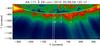 |
Fig. 1 Context map of a south polar coronal hole from AIA/SDO 171 Å passband. The continuous white line box in off-limb region indicates the selected plume region for which a time–distance intensity map (see Fig. 3) and a frequency–distance Fourier power map (see Fig. 6) are obtained. Different small boxes indicate the individual spatial locations chosen for detailed analysis. To make the far off-limb structures visible, a radial enhancement filter is applied on the image. |
In astronomy, a collection of unresolved motions in space or time, or dynamical oscillations having a broad-band spectrum of frequencies without any dominant frequency, are termed as turbulence (Cranmer 2007). In turbulence, the spectrum of variable fields are known to obey a power-law distribution over a range of scales (Kolmogorov 1941; Iroshnikov 1964; Kraichnan 1965). Turbulence is ubiquitous in the Sun and heliosphere and power-law distributions are observed in the solar atmosphere, solar wind, and interplanetary medium (detailed in Bruno & Carbone 2005; Petrosyan et al. 2010). Turbulence can play an important role in wave excitation. Samadi & Goupil (2001) developed theoretical formalism of excitation for stellar p-modes by turbulent convection and applied it to the Sun (Samadi et al. 2001). Moreover, Farmer & Goldreich (2004) indicated the importance of background turbulence in the damping of MHD waves. Thus, turbulence can be considered as an important process to study excitation and damping mechanisms of MHD waves in the upper solar atmosphere.
In this paper, we focus on polar coronal holes, which are considered as a source regions of high-speed solar wind streams (Krieger et al. 1973). In this region, field lines are open and almost radial, which allows us to trace them easily for detailed study. For more details about the region, see the review by Cranmer (2009). We demonstrate the presence of propagating waves along the coronal structures in the off-limb region (Sect. 3.1). We create Fourier power maps in different frequency ranges of the coronal hole (Sect. 3.2) and choose one plume structure for detailed study (Sect. 3.3). We investigate the dissipation of propagating waves after taking the effects of gravitational stratification and field line divergence into account (Sect. 3.4). Further, we discuss the origin and source of various results presented in the previous sections (Sect. 3.5), and, finally, a summary of our results are presented (Sect. 4).
2. Observations
AIA/SDO provides full-disk solar images in seven EUV and three UV-visible channels covering a temperature range from 6 × 10⁴ K to 2 × 10⁷ K. The instrument records continuous images of the Sun with spatial resolution of 1.5″ and temporal resolution of 12 s (Lemen et al. 2012). We chose a three hrs time sequence in 171 Å and 191 Å passbands on 2010 June 29 between 06:00 UT to 09:00 UT from AIA/SDO in the south polar coronal hole. Emission in these two passbands mainly comes from Fe ix/x and Fe xii ions. All the images were calibrated, co-aligned, and rescaled to a common 0.6″ plate scale using aia_prep.pro routine available in the SolarSoft (SSW). All the images were rebinned over 2 × 2 spatial pixels to improve the signal strength in the off-limb region. Figure 1 shows the region of the south polar coronal hole analysed in this study. A radial filter was applied to the image to enhance the visibility of coronal structures in the far off-limb region.
3. Results and discussion
3.1. Propagating disturbances in the polar coronal hole
In the south polar coronal hole, several coronal structures such as plumes and inter-plumes can be identified from the intensity contrast (see Fig. 1). At these locations, artificial slits were traced from the near limb region to close to the end of the AIA/SDO field of view (FOV). The width of the slits were kept about 12″ in the solar-X direction. Time–distance maps were created using the intensity along these slits. One such plume structure marked in Fig. 1 was chosen for further detailed study. Average intensity decrease along the plume structure were obtained in AIA 171 Å and 193 Å passbands and fitted with exponential function I = I0exp ( − h/HI) + c using the MPFIT routines (Markwardt 2009) to obtain the intensity decay scale heights (HI) in both the passbands (see Fig. 2). The obtained intensity scale heights were 32 Mm and 29 Mm for AIA 171 Å and 193 Å passbands, which leads to the density scale height to be 64 Mm and 58 Mm for both the passbands as I ∝ ρ2.
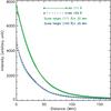 |
Fig. 2 Average intensity decrease with height along the plume structure marked in Fig. 1. Intensity decrease are fitted with exponential function to obtain the intensity decay scale heights in AIA 171 Å and 193 Å passbands and are labelled in the figure. |
In Fig. 3, we show the presence of propagating disturbances from the time-distance map along the plume structure obtained in AIA 171 Å and 193 Å passbands. Time-distance maps are created after subtracting 100-point running average in time (≈20 min) from each spatial pixels along the artificial slit. The slope of propagating ridges provide a speed of propagation that were measured about 116.5 ± 4.6 km s-1 and 149.7 ± 6.4 km s-1 in 171 Å and 193 Å passbands. Almost all the structures show the presence of propagating disturbances reaching very far out in the corona with the dominant period range between 10 min to 25 min, as also reported by Krishna Prasad et al. (2011) in different AIA channels. Measured propagation speeds are temperature dependent. The ratio of propagation speed between 193 Å and 171 Å channels is about 1.29 whereas the ratio of the peak temperature of dominant contributing ions in the two filters can be anywhere in the range 1–1.58–1.99–2.24 in a coronal hole (dominant ion contributing in 171 Å channel is Fe ix whereas that in 193 Å channel are Fe ix, Fe x, Fe xi, and Fe xii, O’Dwyer et al. 2010). These two ratios are close enough to follow the relation of acoustic waves Cs ∝ T1/2 (Priest 1984). Banerjee et al. (2009) interpreted propagating disturbances in the coronal hole in terms of slow magneto-acoustic waves based on their temperature dependent propagation speeds from the spectroscopic data. Recently, Krishna Prasad et al. (2011) and Kiddie et al. (2012) also found similar temperature dependent propagation speeds of intensity disturbances from AIA/SDO imaging observations and again interpreted them in terms of slow magneto-acoustic waves. Uritsky et al. (2013) developed a new data analysis methodology to measure the speed of propagating disturbances. They found that the speed of these disturbances increases with the temperature and follows the square-root dependence as predicted for propagating slow magneto-acoustic waves. Gupta et al. (2012) performed a detail line profile study of propagating disturbances in a polar coronal hole and found them to be consistent with propagating slow magneto-acoustic waves. Henceforth, propagating disturbances observed in the coronal hole with similar properties in this study can also be attributed to the presence of propagating slow magneto-acoustic waves.
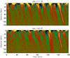 |
Fig. 3 Processed time-distance intensity maps of plume region marked in Fig. 1 summed over 12″ width in the X-direction. The quasi-periodic (in the range 10–20 min) propagating disturbances are observed with speed ≈116.5 ± 4.6 km s-1 in 171 Å (top panel) and ≈149.7 ± 6.4 km s-1 in 193 Å (bottom panel) AIA/SDO channels. Disturbances are reaching very far in the off-limb corona. |
 |
Fig. 4 Wavelet results for the locations at a distance of 2.6 Mm (left panels) and 20.2 Mm (right panels) from the limb brightening height for a plume region marked in Fig. 1 in AIA 171 Å channels. In each set, the top panels show the trend subtracted (100-point running average) intensity variation with time. The bottom-left panels show the colour-inverted wavelet power spectrum with 99% confidence-level contours, while the bottom-right panels show the global wavelet power spectrum (wavelet power spectrum averaged over time) with 99% global confidence level drawn. The periods P1 and P2 at the locations of the first two maxima in the global wavelet spectrum are shown above the global wavelet spectrum. |
3.2. Fourier power maps of the polar coronal hole
The result presented in Sect. 3.1 provides evidence of propagating slow magneto-acoustic waves, which reach very far out in the off-limb corona. Upon performing the wavelet analysis (Torrence & Compo 1998) at two different heights (2.6 Mm and 20.2 Mm from the limb brightening region, Fig. 4), we found clear presence of both small (≈5 min) and long period (≈20 min) oscillations at lower heights whereas at larger heights we found only long period (≈20 min) oscillations. This may indicate some period or frequency dependent nature of detection length of wave propagation in the solar atmosphere, where detection length is defined as length over which oscillations are visible above certain noise level (De Moortel et al. 2002b). Thus, in this section, we look for distance travelled (detection length) by observed propagating waves in the polar coronal hole in different period/frequency ranges. To achieve this in detail and for a wide range of frequencies, we obtained Fourier power for all the spatial pixels in the polar coronal hole. While applying the Fourier transform (FT) on each spatial pixel, we subtracted the mean value from the original time series curves without any further trend subtraction or filtration so as to avoid any kind of bias effect. Thus, a 3D datacube of Fourier powers were obtained in the polar coronal hole. While analysing the Fourier powers in off-limb corona, we need to consider the effect of fall off in brightness with height. Brightness depends upon density, which decreases with height due to gravitational stratification in the off-limb corona. Wave propagation in the off-limb corona will perturb the density residing on the top of density fall. The Fourier power of an oscillation at a particular frequency completely depends upon its oscillation amplitude irrespective of the mean value on which it oscillates. Thus, the Fourier power of an oscillation with absolute amplitude between any ± n will always be the same irrespective of the oscillation sitting on the top of any mean intensity. Therefore, beacause of fall off in brightness with height, Fourier powers of oscillations will remain constant if absolute amplitude of oscillations are constant with height.
We created several frequency windows (ranges) to analyse the 2D Fourier power map of the polar coronal hole in several frequency bins. We divided the frequency scale in three parts to study (i) long periods (periods between 16 min to 45 min); (ii) intermediate periods (periods between 6 min to 15 min); and (iii) short periods (periods between 3 min to 6 min). We summed the Fourier powers in the respective frequency bins and obtained the Fourier power maps of the polar coronal hole in those frequency/period ranges and plotted them in Fig. 5.
Figure 5 clearly shows that long-period waves reach very large distances in the corona whereas short-period waves reach very low distances in the corona for the same Fourier power level. At first glance, this can be interpreted as a clear indication of frequency dependent detection length of these waves. Longer period waves have longer detection length as compared to short period waves, however, one needs to examine the nature of damping length (distance over which the wave amplitude has an e-folding decay, De Moortel et al. 2002b) with frequency (period) before arriving at any conclusion. More analysis on damping length of these waves are presented in the next sections. Moreover, Fourier power spectra at individual spatial locations also show the presence of power peaks at different frequencies and confirm the presence of oscillatory signatures as seen in Figs. 3 and 4. Details about the individual Fourier power spectra are discussed later in Sect. 3.5. From these power maps, it is also noted that 171 Å power contours provide finer details of the coronal structures whereas 193 Å power contours are relatively wider in width. This could be a result of the wider temperature response of 193 Å filter in the coronal hole region, as reported by O’Dwyer et al. (2010).
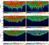 |
Fig. 5 Fourier power map (power in logarithmic scale) of south polar coronal hole obtained from 171 Å (left panels) and 193 Å passbands (right panels) of AIA/SDO in different period ranges as labelled. White line contours are plotted at the same Fourier power level (≈1.7 in log scale) in all the panels of 171 Å and 193 Å passbands. Location of solar limb is also over-plotted with continuous yellow line in all the panels. |
3.3. Frequency-distance Fourier power map of propagating disturbances
In order to study the distance travelled (detection length) by waves with different frequencies (periods), we analysed the same plume structure selected for the time-distance map in Fig. 3 and marked with a pair of continuous straight lines in the off-limb region of Fig. 1. In Fig. 6, we show the Fourier power distribution with frequency and distance above the limb of the analysed plume region. An isocontour (continuous yellow line) of Fourier power is over-plotted to show the distance travelled by waves at different frequencies. The nature of contour indicates that the decrease of detection length is very rapid with respect to frequency. Power peaks observed near 1 mHz (≈17 min) and between 3−5 mHz (≈3−6 min) frequency ranges show different length scales of distance travelled. This rapid decrease may explain the detection of only longer period waves in the far off-limb corona with EIT/SOHO (e.g. DeForest & Gurman 1998) and UVCS/SOHO (Ofman et al. 1997) instruments, and studies further far in the heliosphere (see review by Banerjee et al. 2011). The observed detection length of oscillations with respect to frequency can be visualised from the contour plot in Fig. 6.
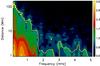 |
Fig. 6 Frequency-distance Fourier power map (power in logarithmic scale) for plume region marked in Fig. 1 summed over 12″ width in X-direction. The over-plotted continuous yellow line contour indicates the same Fourier power level (≈0.99 in log scale) with frequency. Y-axis (distance axis) is in log scale. |
Observed periods found here ranges from a few minutes to several minutes. The acoustic cut-off frequency for the corona with a temperature of 1 MK is about 70 min (Ofman et al. 1999). As periods of oscillations analysed in this study are clearly below 70 min, if these waves were generated in the low corona, they could easily propagate along the field lines and detected up to far distances as found in this study. There are recent reports, however, providing evidence of longer period waves also present at lower solar atmospheric heights of the quiet-Sun network regions (Gupta et al. 2013). Thus, the possibility of the origin of longer period waves observed in the corona to be at lower solar atmospheric heights cannot be ruled out. In those case, however, the longer period waves above the acoustic cut-off of the respective layer of solar atmosphere will be able to propagate further only along the inclined field lines. These longer period waves could be the result of some longer time scale photospheric motions, which may be verified by observing the spectrum of photospheric motions below the plume structures as suggested by Ofman et al. (1999).
3.4. Effect of area divergence, gravitational stratification and other parameters
In the Sects. 3.2 and 3.3, we showed the possible frequency dependent nature of detection lengths of propagating slow magneto-acoustic waves in the solar corona. However, effect of various coronal parameters should be taken into account to conclude on any frequency dependent nature of damping lengths.
As mentioned earlier, Fourier power at a frequency depends upon the absolute amplitude of oscillation rather than on the relative amplitude. From the Figs. 5 and 6, we can see that the Fourier powers in different frequency ranges decrease with height, and thus, indicate that the amplitude of waves are decreasing with height. This decrease in amplitudes are the result of damping of waves in the solar corona due to various mechanisms.
In the solar atmosphere, because of gravitational stratification and magnetic field divergence, absolute wave amplitude of density perturbation decreases while the relative wave amplitude increases with height in the off-limb corona because of decrease in the background density (Ofman et al. 1999). This implies that FT value at a frequency due to wave propagation, in principle, will decrease with height. However, one should be careful that decreases in the FT values with height due to stratification and area divergence are not actual dissipation of waves as there is no dissipative mechanisms involved. These are purely a geometrical effect. Thus, both effects combine together reduces the FT values quickly with height and take a form proportional to both. Following Ofman et al. (1999), equilibrium density in the solar atmosphere is given as ![Mathematical equation: \begin{equation} \rho = \rho_0 \exp\left[-\frac{R_\odot}{H}\left(1-\frac{R_\odot}{r}\right)\right], \label{eq:density} \end{equation}](/articles/aa/full_html/2014/08/aa23200-13/aa23200-13-eq21.png) (1)and approximate change in density due to wave propagation as
(1)and approximate change in density due to wave propagation as ![Mathematical equation: \begin{equation} {\rm d}\rho \sim \frac{R_\odot}{r} \exp\left[-\frac{R_\odot}{2H}\left(1-\frac{R_\odot}{r}\right)\right], \label{eq:cdensity} \end{equation}](/articles/aa/full_html/2014/08/aa23200-13/aa23200-13-eq22.png) (2)where R⊙ is the solar radius, H is the density scale height ≈61 Mm for T = 106 K, and r = R⊙ + h (h is height above solar limb).
(2)where R⊙ is the solar radius, H is the density scale height ≈61 Mm for T = 106 K, and r = R⊙ + h (h is height above solar limb).
As a measurable quantity, intensity I ∝ ρ2, thus, the change in intensity due to wave propagation will be obtained as ![Mathematical equation: \begin{equation} {\rm d}I\propto 2\rho {\rm d}\rho ~~\propto \frac{R_\odot}{r} \exp\left[-\frac{3R_\odot}{2H}\left(1-\frac{R_\odot}{r}\right)\right]\cdot \label{eq:dint} \end{equation}](/articles/aa/full_html/2014/08/aa23200-13/aa23200-13-eq28.png) (3)As FT values depend upon amplitude of oscillations (dI) at different frequencies, in Fig. 7 we show the decrease of FT values with height for the analysed plume region in different frequency ranges. This variation of FT values obtained in different frequency ranges with height can be compared with the expected decrease with height after taking the effect of stratification and area divergence into account as obtained in Eq. (3).
(3)As FT values depend upon amplitude of oscillations (dI) at different frequencies, in Fig. 7 we show the decrease of FT values with height for the analysed plume region in different frequency ranges. This variation of FT values obtained in different frequency ranges with height can be compared with the expected decrease with height after taking the effect of stratification and area divergence into account as obtained in Eq. (3).
Upon choosing the reference FT value at very low height to obtain its decrease with height as per Eq. (3) in different frequency ranges, we found that the observed values were decreasing much more rapidly than those expected from Eq. (3). Thus, we chose the reference value at a distance around 10 Mm from the limb to obtain the curves according to Eq. (3) for all the frequency ranges. By comparison, we found that the FT values in all the frequency ranges were still smaller than those predicted by Eq. (3). FT values at farther higher heights flatten outs which indicates the appearance of white noise at those heights in the respective frequency ranges. Thus, from Fig. 7, it is clear that, in all the frequency ranges, the FT values are decreasing more rapidly with height than that expected from the stratification and area divergence together as per Eq. (3). This may indicate the dissipation of slow waves with height due to various other parameters present.
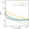 |
Fig. 7 Variation of Fourier transform values with height in different period (frequency) ranges as marked with different colours. Dotted lines indicate the observed decrease with height whereas continuous lines are those obtained after taking Eq. (3) into account. |
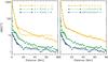 |
Fig. 8 Variation of Fourier transform values with height in different period (frequency) ranges as marked with different colours. Dotted lines are observed decrease with height whereas continuous lines are fit applied to obtain dissipation lengths, as per Eq. (6), using full height range (left panel), and in two height ranges (0–10 Mm and 10–70 Mm, right panel). The obtained dissipation lengths in two different height ranges are summarised in Table 1. |
The rapid decrease of FT values with height in comparison to Eq. (3) indicate the presence of additional physical components that result in the real dissipation of wave energy. These could be due to major damping parameters known such as thermal conduction, compressive viscosity, radiation and other effects, or it could be due to a combination of several effects. Propagation and damping of slow magneto-acoustic waves in solar atmosphere are very well studied theoretically. The models of Nakariakov et al. (2000), De Moortel & Hood (2004), and Klimchuk et al. (2004) for coronal loops indicate thermal conduction to be the dominant dissipative mechanism among all. Ofman et al. (1999, 2000) investigated the role of non-linear steepening of waves leading to dissipation via compressive viscosity in polar plumes using 1D and 2D MHD codes. De Moortel et al. (2002a) found that thermal conduction could alone explain the damping of slow magneto-acoustic waves observed in coronal loops by TRACE. They also highlighted the relation between wave period (frequency) and damping length of slow waves (Fig. 7a of De Moortel et al. 2002a).
Equation (3) can be further simplified using the geometric series approximation 1/(1 − x) = 1 + x + x2 + x3 + ... for | x | < 1, here x = −h/R⊙ with h being very small as compared to R⊙, and thus, ignoring the higher order terms and taking R⊙/r ≈ 1, we find ![Mathematical equation: \begin{equation} {\rm d}I\propto\frac{R_\odot}{r} \exp\left[-\frac{3R_\odot}{2H}+\frac{3R_\odot^2}{2H(R_\odot+h)}\right] ~~\propto \exp\left( - \frac{3h}{2H} \right)\cdot \label{eq:dintc} \end{equation}](/articles/aa/full_html/2014/08/aa23200-13/aa23200-13-eq36.png) (4)This is in agreement with the findings of De Moortel et al. (2002a) and Klimchuk et al. (2004) for the observed intensity perturbation of an acoustic wave propagating along the loop.
(4)This is in agreement with the findings of De Moortel et al. (2002a) and Klimchuk et al. (2004) for the observed intensity perturbation of an acoustic wave propagating along the loop.
Upon finding the evidence of true dissipation of slow waves, we can further obtain the dissipation length scale in this case. We thus add the effect of dissipation by multiplying the right-hand side of Eq. (4) by e−h/2Hd, where Hd is termed as ‘dissipation length’ for wave energy as suggested by Klimchuk et al. (2004). We find
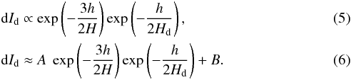 Where A and B are appropriate constants and H ≈ 61 Mm. Thus, we obtained the dissipation length in different frequency ranges, by fitting the FT values in different frequency ranges as per the Eq. (6) using the MPFIT routines (Markwardt 2009). First, we fitted the FT values for heights up to 70 Mm in different frequency ranges and found that a single fit over whole height range did not represent a good fit (left panel of Fig. 8). Therefore, as we found earlier that FT values were decreasing much more rapidly in the first 10 Mm distance, we divided the fit into two height ranges viz between 0–10 Mm and 10–70 Mm. The resultant fits are presented in right panel of Fig. 8 and dissipation lengths we obtained in different period (frequency) and height ranges are summarised in Table 1.
Moreover, we also searched for any evidence of non-linearity in intensity oscillations at several heights. The relative amplitude of oscillations were about 8–10% for the heights within first 10 Mm whereas that increased up to 13–15% beyond 10 Mm distance. These relative amplitudes of oscillations are within the limits of linearity, thus, dissipation of waves via compressive viscosity may not be the dominant mechanism here.
Another possible dissipative mechanism that may lead to dissipation of these waves could be thermal conduction. Klimchuk et al. (2004) and Krishna Prasad et al. (2012) found that dissipation length due to thermal conduction is inversely proportional to the square of frequency (or directly proportional to the square of period) of wave propagation, i.e. Hd ∝ 1 /f2 (or Hd ∝ P2). In our analysis, dissipation lengths obtained for wave propagation as summarised in Table 1 indicate that there might exist some correlation between the dissipation lengths we obtained between 10−70 Mm height range and periods (frequencies) of wave propagation, and, more likely, it appears that dissipation lengths are in direct (inverse) relation with periods (frequencies). No such relationship can be inferred from the dissipation lengths obtained at the lower height range (0−10 Mm). Thus, the obtained results may indicate the presence of thermal conduction to be one of the dominant dissipative mechanism for the dissipation of slow waves at least in the height range of 10−70 Mm for the observed plume structure. At the same, however, presence of other dissipative mechanisms showing relation between dissipation length and period (frequency) of wave propagation cannot be ruled out.
Evidence of damping of slow magneto-acoustic waves were also found in the fan-like coronal loops by Krishna Prasad et al. (2012) and suggested thermal conduction to be the dominant damping mechanism for the longer period slow magneto-acoustic waves. Marsh et al. (2011), however, found thermal conduction to be insufficient and magnetic field line divergence as the dominant factor in damping of slow waves with long-period oscillations in relatively cool and open structures of active regions. Here, we found two distinct dissipation length scales of wave amplitude decay at two different height ranges (between 0–10 Mm and 10–70 Mm) along the observed plume structure and the causes of those at lower heights are not clear. We would like to point out that damping lengths of slow wave propagation as a result of due to dissipation from thermal conduction is of the order of 200–1000 Mm for the periods observed here (see De Moortel et al. 2002a; Marsh et al. 2011). The detection lengths found by De Moortel et al. (2002b), however, were of the order of 10 Mm for 5 min period propagating slow waves and those found by Wang et al. (2009) were of the order of 70 Mm for the longer period waves. Clearly, damping lengths obtained from the forward modelling of thermal conduction are far too large to be able to explain the observed dissipation lengths of the order of a few Mm at different heights in the solar corona (see Table 1). A slightly enhanced thermal conductivity (four times of standard coronal value) can explain the smaller values of damping length as suggested by De Moortel et al. (2002a). Thus, these observed dissipation lengths of slow waves may place a quantitative constraint on the theoretical models of slow wave propagation and dissipative parameters in the solar corona.
Observed dissipation lengths of wave propagation in different period (frequency) ranges and at different heights.
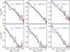 |
Fig. 9 Fourier power distribution with frequency for locations 1–6 marked in Fig. 1. Thin continuous lines represent Fourier powers obtained from original signal (after subtracting mean values). Powers were fitted with power-law distribution with spectral indices (αn) as labelled and are over-plotted with the thick continuous lines. |
Summary of distribution parameters at various locations.
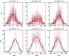 |
Fig. 10 PDFs obtained for intensity fluctuations at locations 1–6 marked in Fig. 1. PDFs were fitted with Gaussian distributions and are over-plotted with continuous blue lines. |
3.5. Turbulence power spectra in the polar coronal hole
From the various Fourier power maps and plots presented in the paper, we found that FT values at the base of the originating point of waves, and at further higher heights in the solar corona are different in various frequency ranges. Basically, the FT values at low frequencies were higher than those at high frequencies at similar heights, which made low frequency waves travel longer distances in the off-limb corona. In this section, we discuss the origin of such behaviour by analysing individual Fourier power spectra at several spatial locations in the polar coronal hole. Figure 9 shows the variation of Fourier power spectra with frequency at locations 1−6 in the polar coronal hole that are marked in Fig. 1. The locations chosen close to the limb are about 30″ away from the limb whereas those farther away are separated by about 35″ in radial direction from the first location. We chose these selected lower height locations because the Fourier powers are present over the whole range of frequencies, from low to high ranges, only at these heights (see Fig. 5). We chose different polar structures to perform our analysis so as to demonstrate consistent results in multiple structures. The power spectra we obtained are frequency dependent and have 1 /fα dependence, where α is the spectral power index. Individual power spectra at different locations were fitted with spectral indices, as labelled in the panels, and are summarised in Table 2. The values of α are very close to 5/3, and may indicate the presence of a Kolmogorov type power spectra (the nearly stationary regime of classical Kolmogorov turbulence; Kolmogorov 1941) which is usually observed in the solar wind turbulence (Bruno & Carbone 2005). These power spectra do not only show frequency dependence, but also show few small power peaks that resulted from oscillatory signatures due to waves propagation at those frequencies (power peaks are also observed in the wavelet plots, Fig. 4). In our study, an analysis was performed over a three-hour time sequence, which resulted in frequencies in the range 0.1 mHz to 40 mHz. These spectra fit very well for frequencies between 0.3 mHz to 4.0 mHz, and beyond that white noise (flat spectra) start to appear depending upon the signal strength. Because of this 1 /fα dependence, power spectra are always dominated by low-frequency oscillations, which were used to be removed by trend subtraction in the earlier studies. Low-frequency dominance is independent of length of time sequence and exists over all the time-scales. The most appropriate example of this phenomena would be of solar cycle. If one takes the power spectrum (FT) of the raw time sequence of sunspot numbers over hundreds of years without any sophistication, the well-known 11-year period of sunspot numbers do not show up as sharp peak in the power spectrum (Mandelbrot & Wallis 1969). The peak gets smeared out in a strong power-law distribution which rises towards low frequencies (Press 1978).
The power spectra shown in Fig. 9 are generally called “flicker noise/spectra” in astronomy (Press 1978) and are observed in interplanetary medium (detailed in Bruno & Carbone 2005; Petrosyan et al. 2010) in the frequency ranges mainly between 10-6 Hz to 10-3 Hz with different α values. The 1 /fα dependent power spectra are interpreted due to the presence of MHD turbulence (see the review by Tu & Marsch 1995). Recently, Bemporad et al. (2008) and Telloni et al. (2009a) showed a similar kind of power spectra in Lyα observations from UVCS/SOHO in the polar coronal hole near the Sun at around 2 R⊙ and in the outer solar corona at 1.7 R⊙, covering the fast and slow wind regions, respectively. Telloni et al. (2009b) found similar density fluctuations in slow and fast wind streams from the outer solar corona to interplanetary space. Moreover, the photospheric magnetic field measured from MDI/SOHO also shows similar spectra (Matthaeus et al. 2007). Reardon et al. (2008) found the presence of a power-law distribution of oscillatory power with frequency in the chromosphere with spectral indices (α) 2.4 and 2.5 in the network and fibril regions, respectively. We still need to perform more work to find the origin of 1 /fα spectra either in corona or elsewhere such as in photosphere or chromosphere. Height and structural dependence of spectral indices (α) are still unclear and detailed analysis needs to be performed to achieve any conclusive result. Here we report, however, the presence of 1 /fα spectra in near the Sun’s polar coronal environment (within 1.1 R⊙) from intensity (≈density) fluctuations in time, which were reported earlier for higher heights (e.g. Bemporad et al. 2008; Telloni et al. 2009a,b).
Statistics of intensity fluctuations are important in the study of turbulence. The probability density function (PDF) of intensity fluctuations resulting from turbulence are expected to have near-Gaussian distribution (not truly Gaussian), however, at small scales distribution can be highly non-Gaussian (page 51, Frisch 1995). Recently, Leonardis et al. (2012) performed the probability distribution analysis on intensity fluctuations of solar prominence in space and time domain and found non-Gaussian and near-Gaussian distributions in both domains, which were attributed to the presence of MHD turbulence. Reardon et al. (2008) found chromospheric PDFs to be non-Gaussian and photospheric PDFs to be nearly Gaussian in the quiet-Sun region, which were attributed to intermittent phenomena associated with a turbulent cascade.
To study nature of the distribution of intensity fluctuations in the polar coronal hole, we plot PDFs obtained at locations 1–6 in Fig. 10. The mean value of intensity fluctuations were subtracted before obtaining the PDFs at all locations. We fitted the PDFs with standard Gaussian function and over-plotted for comparison. Gaussian profiles represent individual PDFs quite fairly. To verify any deviation from Gaussanity, we estimate higher moments of intensity fluctuations. We measured the third and fourth moment of probability distribution viz., skewness and kurtosis. Skewness is the measure of symmetry about the mean value whereas kurtosis is that of peakedness. For a Gaussian distribution, skewness and kurtosis are zero and three, respectively. We calculated skewness and kurtosis for all the locations using IDL routines skewness.pro and kurtosis.pro respectively, and the parameters we obtained are presented in Table 2 (IDL routine calculates excess kurtosis defined as k¯ = k–3). Figure 10 and values presented in Table 2 indicate that distribution of PDFs are near-Gaussian. There could be, however, uncertainties in intensity measurements due to data noise, thus, the observed distribution may be considered as nearly (or almost) Gaussian. This departure from non-Gaussanity is expected as observations are integrated, line-of-sight intensity measurements. The line-of-sight measurements are still expected to capture qualitative features of turbulence such as power-law distribution and non-Gaussian fluctuations, however, the measurements may not lead to the similar theoretically predicted results. Leonardis et al. (2012) found power law distributed power spectra and similar near-Gaussian distribution of intensity fluctuations in the time domain from the observations of solar prominence where the quantitative signatures of turbulence were found. Based on the results presented in Figs. 9 and 10, and Table 2, which confirm the power-law distribution of the Fourier power spectra and near-Gaussian distribution of intensity fluctuations at several locations, a presence of turbulence in the polar coronal hole may be inferred.
Recently, Cranmer & van Ballegooijen (2005); Cranmer et al. (2007) and Verdini et al. (2010) developed models of self-consistent coronal heating and acceleration of fast solar wind. In these models, convective motions at the foot-points of magnetic flux tubes are assumed to generate wave-like fluctuations that propagate up into the extended corona, partially reflect back, develop into strong magnetohydrodynamic (MHD) turbulence, and then damped by an anisotropic turbulent cascade. In our study, we found the evidence of propagating MHD waves that were getting heavily damped along with the evidence of turbulence. Although the damping mechanisms involved are not so clear, slow wave damping due to thermal conduction, as suggested by Klimchuk et al. (2004), appeared to be a more appropriate mechanism. Singh et al. (2007) found turbulence to be a viable damping mechanism to explain the spatial damping of 5 − 15 min slow mode oscillations observed in quiescent limb prominences. Therefore, the role of turbulence as detected here may not be ignored in the damping of these waves. Another model from Farmer & Goldreich (2004) suggested damping of MHD waves by background MHD turbulence. In this model, the waves propagating along magnetic field lines get distorted upon collisions with turbulent wave packets propagating in the opposite direction, resulting in a cascade to a smaller scale, and thus dissipation. These current models primarily deal with incompressible MHD waves and turbulence, however, the models highlight the importance of MHD turbulence in wave damping. Thus, the obtained signatures of turbulence would be useful input in order to understand the damping of waves even in the incompressible MHD framework. Nevertheless, to explain the current observations in detail, a model dealing with compressible MHD turbulence would be requested.
In this study, we found propagating slow magneto-acoustic waves and the presence of turbulence in the polar coronal hole. Low-frequency waves were found to travel longer distances as compared to high-frequency waves, which were the result of the relatively high power content of the low-frequency waves. Turbulence spectra, which has similar energy distribution with respect to frequency, and were also found in our study, thus, may generate similar power distributed MHD waves. The origin and generation of these waves found in solar corona are, however, still unclear. Recently, Wang et al. (2013) modelled the propagating disturbances in fan-like coronal loops driven by up-flows with repetitive quasi-periodic tiny pulses generated by sporadic heating events (nanoflares) at the coronal base. The energy-frequency distribution of these events follows the power-law scaling with a broadband power-law spectrum. Wang et al. (2013) found that the observed propagating disturbances are mainly signatures of wave propagation as the speeds are consistent with the wave speed. Thus, the power-law distributed disturbances reported in this study may suggest that the propagating disturbances are possibly driven by turbulent flows at the coronal base. Hence, turbulence spectra found in this study could also provide a viable mechanism for triggering of longer period waves in the solar atmosphere.
4. Conclusion
We presented the evidence of propagating slow magneto-acoustic waves in the polar coronal hole. The waves were reaching very large distance in the off-limb region. We obtained a Fourier power map of the polar coronal hole in several frequency ranges. We found that low-frequency waves were reaching very far out in the off-limb region whereas high-frequency waves were confined to only a short distance in the off-limb region. We obtained wave dissipation lengths in different frequency and height ranges. We found that waves were getting heavily damped in the first 10 Mm distance above the limb with a dissipation length of only a few Mm, whereas beyond that waves were damped slowly with dissipation lengths of the order of several tens Mm, which also depends upon the frequencies. Although the exact nature of frequency dependence of dissipation lengths is not clear, their inverse relation may indicate the possibility of wave dissipation due to thermal conduction (Klimchuk et al. 2004), however, the possibility of other dissipative mechanisms can not be ruled out. Moreover, the cause of heavy damping (smaller dissipation lengths) of slow waves in the first 10 Mm distance is unclear. The results we obtained may place a quantitative constraint on the theoretical models of slow wave propagation and dissipative parameters in the solar corona.
Individual Fourier power spectra obtained at several locations, indicated the clear power-law distribution, which may suggest the signature of turbulence in the polar coronal hole. We obtained PDFs of intensity fluctuations at several locations and found those to be near-Gaussian distribution, and suggested them arised due to the presence of turbulence. We report the presence of turbulence (1 /fα) spectra in the near Sun polar coronal environment (within 1.1 R⊙) from intensity fluctuations in the time domain, which were reported earlier for higher heights (Bemporad et al. 2008; Telloni et al. 2009a). The presence of turbulence could be important in excitation and damping of waves in the polar coronal hole (Stein 1967; Farmer & Goldreich 2004). Because of power-law distribution, low-frequency waves always have high power content as compared to high-frequency waves, and thus, are able to travel longer distances (longer detection lengths) comparatively. Spectral indices obtained from the power-law distribution indicates presence of Kolmogorov like turbulence (Kolmogorov 1941). Results presented in this study may be important in the theoretical modelling of coronal heating and acceleration of the fast solar wind in the coronal holes from the MHD turbulence (Cranmer et al. 2007; Verdini et al. 2010).
Acknowledgments
The author is grateful to the referee for his/her valuable comments and clarifications, which improved the quality of presentation. The author thanks L. Teriaca and S. Solanki for helpful discussions at the earlier stage of this work. The author is thankful to D. Banerjee for his constant support throughout. This work was supported through the INSPIRE Faculty Fellowship of the Department of Science and Technology (DST), Government of India. The data used here are courtesy of NASA/SDO and AIA consortium.
References
- Banerjee, D., Teriaca, L., Gupta, G. R., et al. 2009, A&A, 499, L29 [NASA ADS] [CrossRef] [EDP Sciences] [Google Scholar]
- Banerjee, D., Gupta, G. R., & Teriaca, L. 2011, Space Sci. Rev., 158, 267 [NASA ADS] [CrossRef] [Google Scholar]
- Bemporad, A., Matthaeus, W. H., & Poletto, G. 2008, ApJ, 677, L137 [NASA ADS] [CrossRef] [Google Scholar]
- Berghmans, D., & Clette, F. 1999, Sol. Phys., 186, 207 [NASA ADS] [CrossRef] [Google Scholar]
- Bruno, R., & Carbone, V. 2005, Liv. Rev. Sol. Phys., 2, 4 [Google Scholar]
- Cranmer, S. R. 2007, in Turbulence and Nonlinear Processes in Astrophysical Plasmas, eds. D. Shaikh, & G. P. Zank, AIP Conf. Ser., 932, 327 [Google Scholar]
- Cranmer, S. R. 2009, Liv. Rev. Sol. Phys., 6, 3 [Google Scholar]
- Cranmer, S. R., & van Ballegooijen, A. A. 2005, ApJS, 156, 265 [NASA ADS] [CrossRef] [Google Scholar]
- Cranmer, S. R., van Ballegooijen, A. A., & Edgar, R. J. 2007, ApJS, 171, 520 [Google Scholar]
- De Moortel, I. 2009, Space Sci. Rev., 149, 65 [NASA ADS] [CrossRef] [Google Scholar]
- De Moortel, I., & Hood, A. W. 2003, A&A, 408, 755 [NASA ADS] [CrossRef] [EDP Sciences] [Google Scholar]
- De Moortel, I., & Hood, A. W. 2004, A&A, 415, 705 [NASA ADS] [CrossRef] [EDP Sciences] [Google Scholar]
- De Moortel, I., & Nakariakov, V. M. 2012, Roy. Soc. London Philos. Trans. Ser. A, 370, 3193 [Google Scholar]
- De Moortel, I., Ireland, J., & Walsh, R. W. 2000, A&A, 355, L23 [NASA ADS] [Google Scholar]
- De Moortel, I., Hood, A. W., Ireland, J., & Walsh, R. W. 2002a, Sol. Phys., 209, 89 [NASA ADS] [CrossRef] [Google Scholar]
- De Moortel, I., Ireland, J., Walsh, R. W., & Hood, A. W. 2002b, Sol. Phys., 209, 61 [NASA ADS] [CrossRef] [Google Scholar]
- De Moortel, I., Hood, A. W., Gerrard, C. L., & Brooks, S. J. 2004, A&A, 425, 741 [NASA ADS] [CrossRef] [EDP Sciences] [Google Scholar]
- DeForest, C. E., & Gurman, J. B. 1998, ApJ, 501, L217 [NASA ADS] [CrossRef] [Google Scholar]
- Farmer, A. J., & Goldreich, P. 2004, ApJ, 604, 671 [NASA ADS] [CrossRef] [Google Scholar]
- Frisch, U. 1995, Turbulence. The legacy of A. N. Kolmogorov (Cambridge: Cambridge University Press) [Google Scholar]
- Gupta, G. R., O’Shea, E., Banerjee, D., Popescu, M., & Doyle, J. G. 2009, A&A, 493, 251 [NASA ADS] [CrossRef] [EDP Sciences] [Google Scholar]
- Gupta, G. R., Banerjee, D., Teriaca, L., Imada, S., & Solanki, S. 2010, ApJ, 718, 11 [NASA ADS] [CrossRef] [Google Scholar]
- Gupta, G. R., Teriaca, L., Marsch, E., Solanki, S. K., & Banerjee, D. 2012, A&A, 546, A93 [NASA ADS] [CrossRef] [EDP Sciences] [Google Scholar]
- Gupta, G. R., Subramanian, S., Banerjee, D., Madjarska, M. S., & Doyle, J. G. 2013, Sol. Phys., 282, 67 [NASA ADS] [CrossRef] [Google Scholar]
- Iroshnikov, P. S. 1964, Sov. Astron., 7, 566 [NASA ADS] [Google Scholar]
- Kiddie, G., De Moortel, I., Del Zanna, G., McIntosh, S. W., & Whittaker, I. 2012, Sol. Phys., 279, 427 [NASA ADS] [CrossRef] [Google Scholar]
- Klimchuk, J. A., Tanner, S. E. M., & De Moortel, I. 2004, ApJ, 616, 1232 [NASA ADS] [CrossRef] [Google Scholar]
- Kolmogorov, A. 1941, Akademiia Nauk SSSR Doklady, 30, 301 [Google Scholar]
- Kraichnan, R. H. 1965, Phys. Fluids, 8, 1385 [Google Scholar]
- Krieger, A. S., Timothy, A. F., & Roelof, E. C. 1973, Sol. Phys., 29, 505 [NASA ADS] [CrossRef] [Google Scholar]
- Krishna Prasad, S., Banerjee, D., & Gupta, G. R. 2011, A&A, 528, L4 [NASA ADS] [CrossRef] [EDP Sciences] [Google Scholar]
- Krishna Prasad, S., Banerjee, D., Van Doorsselaere, T., & Singh, J. 2012, A&A, 546, A50 [NASA ADS] [CrossRef] [EDP Sciences] [Google Scholar]
- Lemen, J. R., Title, A. M., Akin, D. J., et al. 2012, Sol. Phys., 275, 17 [NASA ADS] [CrossRef] [Google Scholar]
- Leonardis, E., Chapman, S. C., & Foullon, C. 2012, ApJ, 745, 185 [NASA ADS] [CrossRef] [Google Scholar]
- Mandelbrot, B. B., & Wallis, J. R. 1969, Water Resources Research, 5, 321 [Google Scholar]
- Markwardt, C. B. 2009, in Astronomical Data Analysis Software and Systems XVIII, eds. D. A. Bohlender, D. Durand, & P. Dowler, ASP Conf. Ser., 411, 251 [Google Scholar]
- Marsh, M. S., Walsh, R. W., & Plunkett, S. 2009, ApJ, 697, 1674 [NASA ADS] [CrossRef] [Google Scholar]
- Marsh, M. S., De Moortel, I., & Walsh, R. W. 2011, ApJ, 734, 81 [NASA ADS] [CrossRef] [Google Scholar]
- Matthaeus, W. H., Breech, B., Dmitruk, P., et al. 2007, ApJ, 657, L121 [NASA ADS] [CrossRef] [Google Scholar]
- Nakariakov, V. M., Verwichte, E., Berghmans, D., & Robbrecht, E. 2000, A&A, 362, 1151 [NASA ADS] [Google Scholar]
- O’Dwyer, B., Del Zanna, G., Mason, H. E., Weber, M. A., & Tripathi, D. 2010, A&A, 521, A21 [NASA ADS] [CrossRef] [EDP Sciences] [Google Scholar]
- Ofman, L., Romoli, M., Poletto, G., Noci, G., & Kohl, J. L. 1997, ApJ, 491, L111 [NASA ADS] [CrossRef] [Google Scholar]
- Ofman, L., Nakariakov, V. M., & DeForest, C. E. 1999, ApJ, 514, 441 [NASA ADS] [CrossRef] [Google Scholar]
- Ofman, L., Nakariakov, V. M., & Sehgal, N. 2000, ApJ, 533, 1071 [Google Scholar]
- O’Shea, E., Banerjee, D., & Doyle, J. G. 2006, A&A, 452, 1059 [NASA ADS] [CrossRef] [EDP Sciences] [Google Scholar]
- O’Shea, E., Banerjee, D., & Doyle, J. G. 2007, A&A, 463, 713 [NASA ADS] [CrossRef] [EDP Sciences] [Google Scholar]
- Petrosyan, A., Balogh, A., Goldstein, M. L., et al. 2010, Space Sci. Rev., 156, 135 [NASA ADS] [CrossRef] [Google Scholar]
- Press, W. H. 1978, Comments on Astrophysics, 7, 103 [Google Scholar]
- Priest, E. R. 1984, Solar magneto-hydrodynamics (Dordrecht: Reidel) [Google Scholar]
- Reardon, K. P., Lepreti, F., Carbone, V., & Vecchio, A. 2008, ApJ, 683, L207 [NASA ADS] [CrossRef] [Google Scholar]
- Samadi, R., & Goupil, M.-J. 2001, A&A, 370, 136 [NASA ADS] [CrossRef] [EDP Sciences] [Google Scholar]
- Samadi, R., Goupil, M.-J., & Lebreton, Y. 2001, A&A, 370, 147 [NASA ADS] [CrossRef] [EDP Sciences] [Google Scholar]
- Singh, K. A. P., Dwivedi, B. N., & Hasan, S. S. 2007, A&A, 473, 931 [NASA ADS] [CrossRef] [EDP Sciences] [Google Scholar]
- Stein, R. F. 1967, Sol. Phys., 2, 385 [NASA ADS] [CrossRef] [Google Scholar]
- Telloni, D., Antonucci, E., Bruno, R., & D’Amicis, R. 2009a, ApJ, 693, 1022 [NASA ADS] [CrossRef] [Google Scholar]
- Telloni, D., Bruno, R., Carbone, V., Antonucci, E., & D’Amicis, R. 2009b, ApJ, 706, 238 [NASA ADS] [CrossRef] [Google Scholar]
- Torrence, C., & Compo, G. P. 1998, Bull. Am. Meteorol. Soc., 79, 61 [Google Scholar]
- Tu, C., & Marsch, E. 1995, Space Sci. Rev., 73, 1 [Google Scholar]
- Uritsky, V. M., Davila, J. M., Viall, N. M., & Ofman, L. 2013, ApJ, 778, 26 [NASA ADS] [CrossRef] [Google Scholar]
- Verdini, A., Velli, M., Matthaeus, W. H., Oughton, S., & Dmitruk, P. 2010, ApJ, 708, L116 [NASA ADS] [CrossRef] [Google Scholar]
- Verwichte, E., Haynes, M., Arber, T. D., & Brady, C. S. 2008, ApJ, 685, 1286 [NASA ADS] [CrossRef] [Google Scholar]
- Wang, T. J., Ofman, L., Davila, J. M., & Mariska, J. T. 2009, A&A, 503, L25 [NASA ADS] [CrossRef] [EDP Sciences] [Google Scholar]
- Wang, T., Ofman, L., & Davila, J. M. 2013, ApJ, 775, L23 [NASA ADS] [CrossRef] [Google Scholar]
- Yuan, D., & Nakariakov, V. M. 2012, A&A, 543, A9 [NASA ADS] [CrossRef] [EDP Sciences] [Google Scholar]
All Tables
Observed dissipation lengths of wave propagation in different period (frequency) ranges and at different heights.
All Figures
|
Fig. 1 Context map of a south polar coronal hole from AIA/SDO 171 Å passband. The continuous white line box in off-limb region indicates the selected plume region for which a time–distance intensity map (see Fig. 3) and a frequency–distance Fourier power map (see Fig. 6) are obtained. Different small boxes indicate the individual spatial locations chosen for detailed analysis. To make the far off-limb structures visible, a radial enhancement filter is applied on the image. |
| In the text | |
|
Fig. 2 Average intensity decrease with height along the plume structure marked in Fig. 1. Intensity decrease are fitted with exponential function to obtain the intensity decay scale heights in AIA 171 Å and 193 Å passbands and are labelled in the figure. |
| In the text | |
|
Fig. 3 Processed time-distance intensity maps of plume region marked in Fig. 1 summed over 12″ width in the X-direction. The quasi-periodic (in the range 10–20 min) propagating disturbances are observed with speed ≈116.5 ± 4.6 km s-1 in 171 Å (top panel) and ≈149.7 ± 6.4 km s-1 in 193 Å (bottom panel) AIA/SDO channels. Disturbances are reaching very far in the off-limb corona. |
| In the text | |
|
Fig. 4 Wavelet results for the locations at a distance of 2.6 Mm (left panels) and 20.2 Mm (right panels) from the limb brightening height for a plume region marked in Fig. 1 in AIA 171 Å channels. In each set, the top panels show the trend subtracted (100-point running average) intensity variation with time. The bottom-left panels show the colour-inverted wavelet power spectrum with 99% confidence-level contours, while the bottom-right panels show the global wavelet power spectrum (wavelet power spectrum averaged over time) with 99% global confidence level drawn. The periods P1 and P2 at the locations of the first two maxima in the global wavelet spectrum are shown above the global wavelet spectrum. |
| In the text | |
|
Fig. 5 Fourier power map (power in logarithmic scale) of south polar coronal hole obtained from 171 Å (left panels) and 193 Å passbands (right panels) of AIA/SDO in different period ranges as labelled. White line contours are plotted at the same Fourier power level (≈1.7 in log scale) in all the panels of 171 Å and 193 Å passbands. Location of solar limb is also over-plotted with continuous yellow line in all the panels. |
| In the text | |
|
Fig. 6 Frequency-distance Fourier power map (power in logarithmic scale) for plume region marked in Fig. 1 summed over 12″ width in X-direction. The over-plotted continuous yellow line contour indicates the same Fourier power level (≈0.99 in log scale) with frequency. Y-axis (distance axis) is in log scale. |
| In the text | |
|
Fig. 7 Variation of Fourier transform values with height in different period (frequency) ranges as marked with different colours. Dotted lines indicate the observed decrease with height whereas continuous lines are those obtained after taking Eq. (3) into account. |
| In the text | |
|
Fig. 8 Variation of Fourier transform values with height in different period (frequency) ranges as marked with different colours. Dotted lines are observed decrease with height whereas continuous lines are fit applied to obtain dissipation lengths, as per Eq. (6), using full height range (left panel), and in two height ranges (0–10 Mm and 10–70 Mm, right panel). The obtained dissipation lengths in two different height ranges are summarised in Table 1. |
| In the text | |
|
Fig. 9 Fourier power distribution with frequency for locations 1–6 marked in Fig. 1. Thin continuous lines represent Fourier powers obtained from original signal (after subtracting mean values). Powers were fitted with power-law distribution with spectral indices (αn) as labelled and are over-plotted with the thick continuous lines. |
| In the text | |
|
Fig. 10 PDFs obtained for intensity fluctuations at locations 1–6 marked in Fig. 1. PDFs were fitted with Gaussian distributions and are over-plotted with continuous blue lines. |
| In the text | |
Current usage metrics show cumulative count of Article Views (full-text article views including HTML views, PDF and ePub downloads, according to the available data) and Abstracts Views on Vision4Press platform.
Data correspond to usage on the plateform after 2015. The current usage metrics is available 48-96 hours after online publication and is updated daily on week days.
Initial download of the metrics may take a while.