| Issue |
A&A
Volume 567, July 2014
|
|
|---|---|---|
| Article Number | A77 | |
| Number of page(s) | 14 | |
| Section | Stellar structure and evolution | |
| DOI | https://doi.org/10.1051/0004-6361/201322904 | |
| Published online | 16 July 2014 | |
Hiccup accretion in the swinging pulsar IGR J18245–2452
1
ISDC, Department of AstronomyUniversité de Genève,
Chemin d’Écogia, 16,
1290
Versoix,
Switzerland
e-mail: This email address is being protected from spambots. You need JavaScript enabled to view it.
2
Institute of Space Sciences (ICE; IEEC-CSIC), Campus UAB, Faculty
of Science, Torre C5, Parell, 2a
Planta, 08193
Barcelona,
Spain
3
Anton Pannekoek Institute, University of Amsterdam,
Postbus 94249, 1090 GE
Amsterdam, the
Netherlands
4
INAF-Osservatorio Astronomico di Brera,
via Bianchi 46, 23807 Merate, Lecco, Italy
5
CSIRO Astronomy and Space Science , Locked Bag 194, NSW
2390
Narrabri,
Australia
6
University of Western Sydney, Locked Bag 1797, NSW
1797
Penrith South DC,
Australia
7
International Space Science Institute,
Hallerstrasse 6, 3012
Bern,
Switzerland
8
International Space Science Institute in Beijing,
No. 1, Nan Er Tiao, Zhong Guan
Cun, Beijing,
PR China
9
INAF/Osservatorio Astronomico di Roma,
via Frascati 33, 00040 Monteporzio Catone, Roma, Italy
Received:
23
October
2013
Accepted:
8
May
2014
Abstract
The source IGR J18245–2452 is the fifteenth discovered accreting millisecond X-ray pulsar and the first neutron star to show direct evidence of a transition between accretion- and rotation-powered emission states. These swings provided the strongest confirmation to date of the pulsar recycling scenario. During the two XMM-Newton observations that were carried out while the source was in outburst in April 2013, IGR J18245–2452 displayed a unique and peculiar X-ray variability. In this work, we report on a detailed analysis of the XMM-Newton data and focus on the timing and spectral variability of the source. In the 0.4–11 keV energy band, IGR J18245–2452 continuously switched between lower and higher intensity states, with typical variations in flux by factor of ~100 on time scales as short as a few seconds. These variations in the source intensity were sometimes accompanied by dramatic spectral hardening, during which the X-ray power-law photon index varied from Γ = 1.7 to Γ = 0.9. The pulse profiles extracted at different count-rates, hardnesses, and energies also showed a complex variability. These phenomena were never observed in accreting millisecond X-ray pulsars, at least not on such a short time-scale. Fast variability was also found in the 5.5 and 9 GHz ATCA radio observations that were carried out for about 6 h during the outburst. We interpret the variability observed from IGR J18245–2452 in terms of a hiccup accretion phase, during which the accretion of material from the inner boundary of the Keplerian disk is reduced by the onset of centrifugal inhibition of accretion, possibly causing the launch of outflows. Changes across accretion and propeller regimes have been long predicted and reproduced by magnetohydrodynamic simulations of accreting millisecond X-ray pulsars, but have never observed to produce as extreme a variability as that shown by IGR J18245–2452.
Key words: X-rays: binaries / pulsars: individual: IGR J18245-2452 / stars: neutron
© ESO, 2014
1. Introduction
The X-ray transient source IGR J18245–2452 was discovered in outburst by the hard X-ray imager IBIS/ISGRI (Ubertini et al. 2003; Lebrun et al. 2003) on-board INTEGRAL on 2013 March 28 during monitoring observations of the Galactic Center (Eckert et al. 2013). The preliminary X-ray position provided by ISGRI localized it within the globular cluster (GC) M 28. This association was confirmed by follow-up observations carried out with the Chandra ACIS-I telescope (Garmire et al. 2003) and the Swift/XRT (Burrows et al. 2005). A type I X-ray burst found in the XRT data (Papitto et al. 2013a; Linares 2013) firmly established the source as an accreting neutron star X-ray binary (see also Serino et al. 2013). Pulsations at 3.9 ms were detected in the X-ray flux recored from the source on April 3 and 13 by XMM-Newton,these made IGR J18245–2452 the fifteenth discovered accreting millisecond X-ray pulsar (AMXP). The delays in pulse-arrival times measured by XMM-Newton led to the determination of the source orbital period at 11.03 h (Papitto et al. 2013b, hereafter, Paper I). The measured ephemeris of the system permitted us to securely associate IGR J18245–2452 with a previously known radio millisecond pulsar in M 28 (PSR J1824–2452I), thus making this source the first millisecond pulsar to show direct evidence for swings between regimes with emission powered by either rotation or accretion. This result provided the most secure confirmation to date of the so-called pulsar recycling scenario (Alpar et al. 1982; Radhakrishnan & Srinivasan 1982), according to which old radio pulsars are secularly spun-up to millisecond periods by mass accretion in low-mass binary systems (see Falanga et al. 2005, for the first evidence of a spin-up in AMXP). During the accretion phases, the material inflowing from the companion star forms an accretion disk around the neutron star (NS) and quenches the radio emission previously powered by the rotation of its magnetic field (see Burderi et al. 2003; Archibald et al. 2009, for previous indirect evidence of switches between these two phases in SAX J1808.4–3659 and PSR J1023+0038, respectively).
Log of the XMM-Newton observations.
In addition to these swings between the different emission regimes, IGR J18245–2452 displayed a peculiar variability in the X-ray domain during its 2013 outburst, which was not observed before in other AMXPs. This variability was particularly evident in the two XMM-Newton target-of-opportunity observations carried out during the source outburst. In these observations, the X-ray emission from IGR J18245–2452 repeatedly varied in intensity by a factor of ~100 on time-scales as short as a few seconds. Here, we report on a detailed timing and spectroscopic analysis of the XMM-Newton data, aimed at investigating the nature and origin of the source X-ray variability.
We describe the data analysis technique in Sect. 2 and report all the results in Sect. 3. We present our discussions in Sect. 4 and propose in Sect. 5 that the complex X-ray variability of IGR J18245–2452 arises in an unstable (hiccup) accretion phase, during which the inflowing material is able to penetrate the NS magnetosphere at different latitudes and is often ejected instead of accreted onto the NS because of the onset of the propeller mechanism (Illarionov & Sunyaev 1975; Campana et al. 1998).
2. Data analysis
The log of the XMM-Newton observations we analyzed is provided in Table 1. In the following, we refer to observation ID. 0701981401 as obs1 and to observation ID. 0701981501 as obs2. In both cases, the EPIC-pn was operated in timing mode to attain a timing resolution of 0.03 ms and limit the effect of pile-up1. The two EPIC-MOS cameras were operated in small-window mode and the RGS in standard mode (a thick filter was used for all the EPIC cameras to screen the bright optical light from the globular cluster M 28).
Observation data files (ODFs) from obs1 and obs2 were processed to produce calibrated event lists using the standard XMM-Newton Science Analysis System (v. 13.5.0). We used the epchan, emproc, and rgsproc tasks to produce cleaned event files from the EPIC-pn, the two EPIC-MOS, and the RGS instruments, respectively. No high flaring background time intervals were identified by following the SAS science analysis threads2. Therefore, we retained the entire available exposure time for both obs1 and obs2.
In the EPIC-pn pipeline, we used the rate-dependent pulse height aptitude (PHA) correction to optimize the energy reconstruction of the events3. The EPIC-pn light curves and spectra of the source were extracted by using data from Cols. 26 to 47 (included) of the detector. The corresponding backgrounds were extracted from Cols. 2 to 5 (included). We verified with the SAS task epaplot that when the count rate from the source exceeded ~50 cts/s (0.5–11 keV), the data extracted from the two central columns of the EPIC-pn camera (37 and 38) were affected by pile-up. We corrected for this effect by excluding data from Cols. 37 and 38 during the spectral analysis. The response files for the EPIC-pn were generated taking into account the pile-up problem according to the latest available SAS thread (see above); the default point-spread function model was assumed. EPIC-pn spectra were grouped to have at least 40 counts in each energy bin and to oversample the energy resolution by no more than a factor three. The energy range is limited to 0.6–11 keV, as at lower energies the electronic noise distorts the spectrum4. For the timing analysis, we obtained the photon arrival times at the solar system barycenter using the barycen tool. Following the recommendations of the SAS user manual, we did not attempt to merge the spectra from the two observations characterized by a high count rate, but instead fit them jointly5.
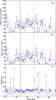 |
Fig. 1 Top panel: XMM-Newton lightcurve of IGR J18245–2452 extracted from obs1 and obs2 in the 0.5–3.5 keV energy band. The vertical dashed line represents the separation between the two observations. Times of obs1 are measured starting from 00:25:22 on 2013 April 04 (TBD). For the second observation the start time is 2013 April 13 at 07:03:06 (TBD; note that times have been shifted by 26.3 ks for plotting purposes). Middle panel: same as before, but in the 3.5–11 keV energy range. This lightcurve was adaptively rebinned to achieve a signal-to-noise (S/N) ratio of 25 in each time bin, while the minimum bins size was set to 200 s (the same binning has been used for the lightcurve in the soft energy band). Bottom panel: hardness ratio (HR) calculated as the ratio of the hard and soft lightcurves. We plot with magenta symbols the time intervals in which the source count rate was lower than 30 cts/s, all the others are given in blue. The points with HR > 0.7 are highlighted with an open circle. |
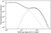 |
Fig. 2 Histogram of the count-rate derived from the combined lightcurves of the two observations (energy range 0.5–11 keV, time bin 1 s). The black solid line represents the total source count-rate. The black dashed line is the sum of two best-fit log-normal distributions, plotted in blue and magenta. |
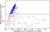 |
Fig. 3 Hardness-intensity diagram built by using all data in obs1 and obs2, which are displayed in Fig. 1 (time bin of 200 s). The black solid line separates the different intensity states: the points represented in magenta and blue have a count rate lower and higher than 30 cts/s, respectively. |
During our analysis, we found that data from the two MOS cameras were strongly affected by pile-up, and using these data did not improve any of the results presented in this paper (we verified a posteriori that all results extracted from the EPIC-MOS data were compatible to within the large uncertainties with those obtained from the EPIC-pn). Therefore, we do not discuss the EPIC-MOS data further.
 |
Fig. 4 Average unfolded spectra of IGR J18245–2452 in obs1 and obs2. Colors refer to the different observations and instruments (red: EPIC-pn obs1; black: EPIC-pn obs2; green: RGS1 obs2; blue: RGS2 obs2; light blue: RGS1 obs1; magenta: RGS2 obs1). The best-fit model is reported in Table 2. We show in the lower panel the residuals from the best fit (see text for details). |
Results of the fits to the average spectra extracted by using all the available exposure time in obs1 and obs2.
The RGS spectra were extracted using standard techniques in the energy range 0.4–1.8 keV, where the calibration of the effective area achieves a 3% accuracy (Kaastra et al. 2009)6. The RGS spectra were rebinned to have 20 counts in each energy bin and obtain a reliable measurement of the absorption column density in the direction of the source. For the hardness-resolved spectra, extracted when the source was dimmer (Sect. 3.2), we combined the two RGS units to increase the signal to noise ration (S/N). The analysis of the O vii triplet, which is detected as a single line in these rebinned RGS spectra, is discussed in Appendix A. Unless otherwise stated, spectral fitting was carried out by using Xspec v12.8 and uncertainties are given throughout our paper at 90% c.l.
3. Results
The lightcurves of the two XMM-Newton observations are shown in Fig. 1. In both observations, the source displays a very prominent variability (all lightcurves are background subtracted and corrected for instrumental effects, e.g., vignetting). During several relatively extended periods of time (a few thousand seconds) the average source intensity was lower than in the rest of the observation, retaining a remarkable variability. A single low-intensity period in obs1 began ~5 ks after the start of the observation and lasted for about 13 ks. Multiple low-intensity periods occurred in obs2. We show in panel (c) of Fig. 1 the hardness ratio (HR) of the lightcurves extracted in the soft (0.5–3.5 keV) and hard (3.5–11 keV) energy bands (see Bozzo et al. 2011, 2013, for details about the HR computation). The HR displayed only a moderate variability during most of the observations (between ~0.3 and 0.5), but underwent rapid and strong variations during the low intensity periods. We folded the lightcurves along the 2.3 orbits covered by XMM-Newton, but no obvious orbital dependency of these phenomena was found.
To characterize the distribution of states at the highest achievable timing resolution
without facing shot-noise limitations, we built the histogram of the source count rate
accumulated in time bins of one second. By inspecting these lightcurves, not shown here for
brevity, we verified that the EPIC-pn count-rate showed switches from ~3–5 cts/s to ≳500 cts/s on time scales as short as a few
seconds (0.5–11 keV). The count-rate histogram is characterized by two broad peaks that can
be described by two log-normal distributions with centroids 5.48 ± 0.06 and 79.5 ± 0.3 cts/s, and widths 2.75 ± 0.04 and 1.74 ± 0.03 cts/s, respectively
( for 121 d.o.f.). Because of this bi-modal
distribution, we draw the separation between dimmer and brighter states at 30 cts/s, where
the two distributions cross. We represent in Fig. 2 the
dimmer state in magenta and marked the others in blue; the
same color coding is maintained for the rest of the paper and is used to identify the two
states. As can be seen in Fig. 1, this division tracks
the intervals of lower activity relatively well, which are characterized by remarkable
swings of the HR and the periods of more intense activity at nearly constant hardness.
for 121 d.o.f.). Because of this bi-modal
distribution, we draw the separation between dimmer and brighter states at 30 cts/s, where
the two distributions cross. We represent in Fig. 2 the
dimmer state in magenta and marked the others in blue; the
same color coding is maintained for the rest of the paper and is used to identify the two
states. As can be seen in Fig. 1, this division tracks
the intervals of lower activity relatively well, which are characterized by remarkable
swings of the HR and the periods of more intense activity at nearly constant hardness.
Figure 3 shows the hardness-intensity diagram (HID) of the source realized by using the same color coding as of Figs. 1 and 2. We note that the blue points form a first branch that is characterized by increasing hardness (HR) as a function of the source intensity and saturates at HR ~ 0.5–0.6; the source spends about 60% of the time in this branch. The magenta points are placed on a second branch that is characterized by an average lower intensity and reaches hardness values of 1.4. The source spends about 40% of the time in this state.
It is important to remark that the picture of the source variability emerging from Fig. 1 is somehow smoothed by the relatively large time bins. When the source light curve is extracted with a time bin of 1 s, the swings are much more pronounced and reach count rates as high as 700 cts/s (Fig. 2). We verified a posteriori that the time intervals corresponding to the magenta and blue states identified using the time bins of 200 s track the different variability pattern of the source reasonably well. This is also valid for other similar choices of binning.
To understand the nature of the HR variations shown by the light curve analysis, we first extracted the average EPIC-pn and RGS spectra (Sect. 3.1). Then, we performed a rate- and HR-resolved spectral analysis for the blue and magenta states separately, using Fig. 3 as guidance (see Sects. 3.2 and 3.3).
Spectral parameters of the best-fit models to the rate-resolved spectra of IGR J18245–2452 during the blue states.
3.1. Average spectrum
The combined RGS+EPIC-pn spectrum (0.4–1.8 keV and 0.6–11 keV) extracted by using the
total exposure time available in obs1 and obs2 is shown in Fig. 4. For both observations, we adopted a spectral model that comprises a
photoelectric absorption with variable abundances of iron and oxygen (tbnew_feo;
Wilms et al. 2001), a thermal Comptonization
(compTH in xspec, the electron temperature was fixed to 50 keV), and
three components due to the accretion disk: a broad Gaussian line, a disk black-body, and
a narrow line corresponding to the non-resolved O vii helium-like triplet (see
Appendix A). Because of EPIC-pn calibration problems related to the energy scale in timing
mode (see also Sect. 2), we introduced in the fit
three Gaussian lines with zero width and centroid energies of 1.5, 1.8, and 2.2 keV. These
energies correspond to pronounced edges in the instrument effective area7. We verified that the relatively large
 for 4067 d.o.f. is mostly due to residual
calibration uncertainties.
for 4067 d.o.f. is mostly due to residual
calibration uncertainties.
The results obtained by separately fitting the spectra of obs1 and obs2 with the model above are similar to within the uncertainties. We therefore report in Table 2 only the results obtained by simultaneously fitting all spectra with the same model.
3.2. Spectral variability
We first investigate the spectral variability of the blue states. To this aim, we extracted four source spectra at different intervals of EPIC-pn count rates higher than 30 cts/s, as reported in Table 3. Simultaneous RGS1 and RGS2 spectra were also extracted and fit together with the EPIC-pn spectra using the same model adopted in Sect. 3.1. With the reduced statistics of these spectra, only the edge at 2.2 keV produced an observable feature in the spectrum, modeled as a zero-width Gaussian line. We introduced in the fits normalization constants to account for calibration uncertainties between the instruments and slight differences in the distribution of source fluxes during the selected time intervals. We checked that all parameters remained compatible to within the uncertainties in the two observations, if left free to vary in the fits. A broad Gaussian line at ~6.4 keV was introduced, similarly as for the average spectrum. The results reported in Table 3 show a significant spectral variability within the blue states, which appears to be caused by a harder asymptotic power-law photon index of the Comptonized spectrum for increasing count rates.
Because the magenta states span a relatively small range of source count rates
(<30 cts/s) while the
source HR displays remarkable variability, we investigated spectral changes in these
states by carrying out a HR-resolved (instead of count-rate-resolved) spectral analysis.
From the results in Fig. 1, we extracted the source
RGS and EPIC-pn spectra of the magenta states in obs1 and obs2 in five HR intervals. In
almost all cases, using a simple absorbed nthComp model resulted in a
very poor fit with evident residuals emerging along the entire 0.4–11 keV energy band. We
therefore tried to improve the fits by adding a black-body, a disk black-body, or a
power-law to the nthComp component. We also used an alternative model
with a power-law and a partially covering absorber. Most of these models gave
statistically equivalent fits to the HR-resolved spectra (see Table 4). The nthComp+power-law model was considered less
suitable because in this case the power-law photon index displayed unphysically large
swings in the different HR-resolved spectra. A model comprising the nthComp
component and a black-body was found to provide a more reliable description of all
spectra with HR < 0.7,
because minor adjustments in the temperature and radius of the black-body were required to
obtain  . An example is shown in Fig. 5. The radius and temperature (2.5 km and 0.4 keV) of the
black-body component are reminiscent of those typically observed from hot spots on NS
surfaces. We verified that adding of a colder and larger thermal component, similar to
that measured during the blue state and associated with the accretion disk around the NS,
did not significantly improve any of the HR-resolved spectra extracted during the magenta
states. The only exception was the spectrum extracted at HR > 0.7. In this case, the parameters of
the thermal component obtained from the fit were compatible with those expected from the
inner boundary of an accretion disk, but the temperature of seed photons in the
nthComp component was far too high (a factor >2) and difficult to be reconciled with
the nearly constant values obtained from the other HR-resolved spectra. We found that a
partially covering model instead provided a reasonable description of this very hard and
peculiar spectrum (Fig. 6). All the results obtained
from the fits to the HR-resolved spectra are summarized in Table 5 and are discussed in Sect. 4.
. An example is shown in Fig. 5. The radius and temperature (2.5 km and 0.4 keV) of the
black-body component are reminiscent of those typically observed from hot spots on NS
surfaces. We verified that adding of a colder and larger thermal component, similar to
that measured during the blue state and associated with the accretion disk around the NS,
did not significantly improve any of the HR-resolved spectra extracted during the magenta
states. The only exception was the spectrum extracted at HR > 0.7. In this case, the parameters of
the thermal component obtained from the fit were compatible with those expected from the
inner boundary of an accretion disk, but the temperature of seed photons in the
nthComp component was far too high (a factor >2) and difficult to be reconciled with
the nearly constant values obtained from the other HR-resolved spectra. We found that a
partially covering model instead provided a reasonable description of this very hard and
peculiar spectrum (Fig. 6). All the results obtained
from the fits to the HR-resolved spectra are summarized in Table 5 and are discussed in Sect. 4.
Reduced χ2 and degrees of freedom of various models for hardness-resolved spectra.
We verified that in none of the count-rate and HR-resolved spectra extracted from the magenta states adding a broad Gaussian iron line significantly improved the fits (most likely because of the relatively limited statistics of these data). The upper limits obtained on the normalization of the line were in all cases largely compatible with the values reported in Table 2. We also checked a posteriori that the spectra extracted at the same count-rate or HR intervals in obs1 and obs2 would give results compatible (despite the larger uncertainties) with those reported in Tables 3 and 5 if fit independently in Xspec.
From the results of the spectral fits we obtained an approximate conversion of the source count-rate into flux and determined the average flux of the blue and magenta states to be 3 × 10-11 erg s-1 cm-2 and 4.0 × 10⁻¹⁰ erg s-1 cm-2. These correspond to a luminosity of 1 × 1035 erg s-1 and 1.4 × 1036 erg s-1 at 5.5 kpc.
3.3. Pulse profile properties
To study the properties of the pulse profile at different flux and energies, we first converted all the photon arrival times into the barycenter of the system, using the ephemeris given in Paper I. Lightcurves were then folded at the 3.9 ms spin period of the source, sampling each profile in 16 phase bins. We investigated the source variability discussed in Sect. 3.2 in more detail by carrying out a count-rate- and HR-resolved analysis of the pulse profiles.
Figure 7 shows the source pulse profiles extracted
during the same time intervals as were used for the rate-resolved spectral analysis (see
Table 3). We fit these profiles by using a
function comprising two Fourier components: 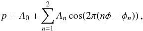 (1)where φ ∈ (0,1) is the normalized
phase. We verified that the addition of higher Fourier components does not significantly
improve the fit. The best fits to the pulse profiles are shown with red lines in
Fig. 7. The parameters determined from the fits are
shown in Fig. 8. The pulsed fraction
(1)where φ ∈ (0,1) is the normalized
phase. We verified that the addition of higher Fourier components does not significantly
improve the fit. The best fits to the pulse profiles are shown with red lines in
Fig. 7. The parameters determined from the fits are
shown in Fig. 8. The pulsed fraction
 increases steadily from 4.0 ± 0.2% to 16.8 ± 0.2% as a function of the source
count rate. The ratio of the amplitude of the second and first harmonic decreases from
0.38 ± 0.06 to
0.10 ± 0.01 as a function of
the count rate. Both the first and the second harmonics underwent a remarkable phase shift
at the highest count rates.
increases steadily from 4.0 ± 0.2% to 16.8 ± 0.2% as a function of the source
count rate. The ratio of the amplitude of the second and first harmonic decreases from
0.38 ± 0.06 to
0.10 ± 0.01 as a function of
the count rate. Both the first and the second harmonics underwent a remarkable phase shift
at the highest count rates.
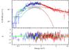 |
Fig. 5 IGR J18245–2452 unfolded spectrum of the soft magenta state (HR < 0.25). The best-fit model (see Table 5) and the residuals from this fit are shown as well. Colors refer to the different observations and instruments (black: EPIC-pn obs1; red: EPIC-pn obs2; green: RGS obs1; blue: RGS obs2). |
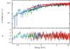 |
Fig. 6 IGR J18245–2452 unfolded spectrum of the hard magenta state (HR > 0.7). The best-fit model (see Table 5) and the residuals from this fit are shown as well. Colors refer to the different observations and instruments (black: EPIC-pn obs1; red: EPIC-pn obs2; green: RGS obs1; blue: RGS obs2). |
Parameters of the best-fit models to the HR-resolved spectra of the magenta using the nthComp plus black-body.
We carried out the same analysis as above for the pulse profiles extracted in the different HR intervals of the magenta states (see Table 5). Pulsations are significantly detected in all HR intervals, but the pulsed fraction was found to be as low as ≃5% (Figs. 9 and 10). The relative contribution of the two harmonics remained constant as a function of the hardness. The phase of the fundamental decreased towards high HR and the first harmonic displayed a jump in the phase for HR > 0.7, which shows a marked morphological evolution.
To summarize these findings and highlight the differences in timing properties between the magenta and blue states, we report in Fig. 11 the results of a timing analysis conducted for each time bin of Fig. 1 instead of by selecting specific intervals in the source count-rate and HR. In the panels (a) and (b) of this figure, we plot the pulsed fraction as a function of HR and total source intensity. Pulsations from the source are significantly detected in each time bin. The pulsed fraction remains virtually constant at ~5% in the magenta states and increases steadily in the blue branch. We also computed the linear correlation coefficient for the different pulse profiles with respect to the average shape. This coefficient is plotted as a function of time and total source intensity in panels (c) and (d). From the comparison to the expected value of the linear correlation coefficient for identical pulses (the yellow band of panel (c)), it is clear that the pulse profiles drastically change their shape especially in the magenta states. We comment on these results in more detail in Sect. 4.
3.4. Aperiodic time variability
We extracted the Fourier power spectra of IGR J18245–2452 in obs1 and obs2 by splitting
them in eight intervals, lasting 3.3 and 7.9 ks, respectively, and averaging the power
spectra evaluated in each of them. We checked that no variability took place on the time
scale set by the orbital motion and discarded from the analysis the frequency bins
corresponding to the first and second harmonic of the pulsations. The two power spectra
were rebinned geometrically by a factor of 1.1. The aperiodic variability of
IGR J18245–2452 is characterized by a power-law noise P(ν) ~
ν− β with β ≃ 1.2 (i.e., flicker
noise). The addition of a flat-top noise component significantly improves the fit of both
power spectra, which we modelled with the function: 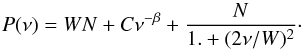 (2)This aperiodic noise component has an RMS
fractional amplitude in the band between 10-4 and 100 Hz that exceeds 90% in both observations. No other features were
detected, even when averaging over shorter time intervals and/or using different rebinning
factors. We also searched for changes of the power spectral shape at different energies,
but found no significant variations with respect to the spectrum extracted over the entire
0.5–11 keV energy band. As an example, we show the power spectral density of obs2 in
Fig. 12 together with the best-fit model. The
best-fit parameters to the power spectra densities of obs1 and obs2 are given in
Table 6.
(2)This aperiodic noise component has an RMS
fractional amplitude in the band between 10-4 and 100 Hz that exceeds 90% in both observations. No other features were
detected, even when averaging over shorter time intervals and/or using different rebinning
factors. We also searched for changes of the power spectral shape at different energies,
but found no significant variations with respect to the spectrum extracted over the entire
0.5–11 keV energy band. As an example, we show the power spectral density of obs2 in
Fig. 12 together with the best-fit model. The
best-fit parameters to the power spectra densities of obs1 and obs2 are given in
Table 6.
In obs1, where the separation between the magenta and blue states is clearer, we carried out a power spectral density (PSD) analysis separately for the two states. We found that the functional shape of the PSD remained unchanged between the two states, but the characteristic frequency of the variability decreased in the magenta states. This can be also inferred also by visually inspecting the lightcurve. PSD fitting reveals that β increases from 1.11 ± 0.02 to 1.27 ± 0.02 when passing from the blue to the magenta states, while the flat-top component remains unvaried within uncertainties.
Best-fit model parameters of the power spectra density extracted by using the entire exposure time available in obs1 and obs2.
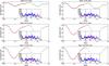 |
Fig. 7 Pulse profiles of the combined obs1 and obs2 extracted during the different count-rate intervals of the blue states as in Table 3. In all panels of this figure, count rates were normalised to the maximum. Pulses are repeated twice for clarity and the red solid lines represent the best fits to the profiles with two sinusoidal functions as described in the text. The insets in each panel show the lightcurves of the two observations in the 0.5–11 keV energy range (as in Fig. 1) with the time intervals used to extract the pulse profiles highlighted in red. |
4. Discussion
We reported on an in-depth analysis of the two XMM-Newton observations carried out in the direction of IGR J18245–2452 during its first observed X-ray outburst.
We first studied the source average X-ray spectrum and showed that the overall spectral
properties of the X-ray emission from IGR J18245–2452 are qualitatively similar to those of
other AMXPs in outburst (Fig. 4, Poutanen 2006; Gilfanov et al.
1998; Gierliński & Poutanen 2005).
Compared with the results we reported in Paper I, including the RGS spectra in this work
allowed us to better constrain the apparent position of the inner accretion disk radius. We
found that rin ≃
66–77 km for an assumed distance to the source of
5.5 kpc. The actual inner radius can be up to a factor ~2 larger when color corrections are
considered (Merloni et al. 2000) and a torque-free
inner boundary condition is applied (Gierliński et al.
1999).
km for an assumed distance to the source of
5.5 kpc. The actual inner radius can be up to a factor ~2 larger when color corrections are
considered (Merloni et al. 2000) and a torque-free
inner boundary condition is applied (Gierliński et al.
1999).
At odds with all the other AMXPs in outburst observed so far (see, e.g., Patruno & Watts 2012, for a recent review), IGR J18245–2452 displayed a very peculiar variability in the X-ray domain and underwent remarkable switches between low- and high-intensity states during both the XMM-Newton observations. The two preferred states were first noticed in the histogram of the source count-rate, which that satisfactorily described only by using two log-normal distributions. The first of the two distributions, marked in magenta, dominates the contribution to the total source count-rate lower than 30 cts/s in the EPIC-pn 0.5–11 keV band. The second distribution, marked in blue, provided the largest contribution at higher count rates. By performing a more detailed analysis on the source light curves, we showed that the HR showed limited changes (~20–30%) around a value of ~0.5 in the blue state, which suggests little spectral variability. During the magenta state, the source intensity was found to be on average a factor of ten lower than in the blue state and characterized by prominent swings in the HR (see Sect. 3). This indicates that significant spectral changes take place in the magenta states. To investigate the origin of the rapid variability, we therefore carried out a count-rate-resolved spectral and timing analysis of the blue states, and an HR-resolved spectral and timing analysis of the magenta states. The results of these analyses are discussed below.
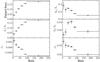 |
Fig. 8 Parameters of the Fourier decomposition of the pulse profiles as a function of the source count-rate in the EPIC-pn data. The different parameters are defined in Eq. (1). Uncertainties are obtained by fitting Eq. (1) to the pulse profiles and given at 1σ c.l. |
In the blue state, the spectral continuum is well described by a thermal Comptonization component plus black-body emission from an accretion disk. Both components remain virtually constant across obs1 and obs2, displaying consistent parameters at different source intensities (we only measured a slight hardening in the photon-index of the Comptonization component, decreasing from Γ ≃ 1.6 to Γ ≃ 1.4 at the highest count rates; see Table 3). In particular, no significant changes are recorded in the equivalent width of the iron line and the absorption column density. These results disfavor any interpretation of the prominent variability of the source intensity observed during the blue state in terms of absorption dips and suggest, instead, that it is due to intrinsic variations of the mass accretion rate onto the NS. These variations regulate the position of the disk inner boundary (see Eq. (3)), pushing it towards the NS surface at high luminosity and enhancing the separation between the inner rim and the NS surface at lower luminosity. By invoking this mechanism, the observed strong correlation of the source pulsed fraction with its X-ray intensity can be explained as it follows: the antipodal spot might become visible, which leads to a reduction of the pulse fraction and an increase of the harmonic content (Beloborodov 2002; Ibragimov & Poutanen 2009; Kajava et al. 2011; Riggio et al. 2011), an annular-shaped accretion stream footprint might shrink (Ibragimov et al. 2011), or variations of the spot latitude might be present (Lamb et al. 2009). Unfortunately, the constraints on rin derived from the different rate-resolved spectra in the blue states are too weak to provide a firm measurement of this effect (see Table 3).
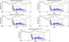 |
Fig. 9 Same as Fig. 7, but here the pulse profiles are extracted for different ranges of the source HR in the magenta states. |
Fits to all the spectra extracted in the magenta state revealed a slight decrease of the
absorption column density, which becomes compatible with the Galactic value in the direction
of the source (2.4 × 10²¹
cm-2; Becker et al.
2003). This is possibly related to the presence of less accreting material in the
surrounding of the NS. The thermal component due to the accretion disk observed in the blue
state was no longer detectable. Instead, a significantly hotter (~0.4–0.7 keV) and more confined (few km)
thermally emitting region was revealed during the spectral fits. Similar regions are usually
associated to hot spots on the NS surface (Gierliński et al.
2002; Gierliński & Poutanen 2005; Papitto et al. 2010, and references therein). To verify
that the accretion disk component was not gone undetected only because of the reduced
statistics of the spectra extracted during the magenta states, we added to the relevant fits
a disk black-body component with a temperature fixed to the value measured in the blue
state. We derived upper limits on  between 9–42 km (at 90% c.l.), which
demonstrates that, if present, such a disk should have been detected in the magenta spectra.
These results agree with the scenario proposed above for the blue states. At the lower
fluxes that characterize the magenta states, the inner boundary of the disk recedes farther
away from the NS surface and thus does not produce a significant contribution to the source
X-ray spectrum. The hot surface of the NS becomes visible along the observer’s line of sight
and dominates the soft X-ray emission from the source.
between 9–42 km (at 90% c.l.), which
demonstrates that, if present, such a disk should have been detected in the magenta spectra.
These results agree with the scenario proposed above for the blue states. At the lower
fluxes that characterize the magenta states, the inner boundary of the disk recedes farther
away from the NS surface and thus does not produce a significant contribution to the source
X-ray spectrum. The hot surface of the NS becomes visible along the observer’s line of sight
and dominates the soft X-ray emission from the source.
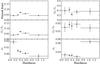 |
Fig. 10 Same as Fig. 8, but for the HR-resolved pulse profiles extracted in the magenta states (Fig. 9). Uncertainties are obtained by fitting Eq. (1) to the pulse profiles and given at 1σ c.l. |
When the inner boundary of the accretion disk recedes beyond a critical value, the so-called propeller effect is expected to set in (Illarionov & Sunyaev 1975). In this regime, accretion onto the NS is (at least) partially inhibited by the rapid rotation of its magnetic field lines, and major changes in the source’s pulsed fraction, pulse profiles, and spectral shape are expected. Interestingly, the pulse fraction of IGR J18245–2452 reaches its minimum in the magenta states (see Figs. 9 and 10) and the corresponding pulse profiles changes drammatically. The latter are nearly sinusoidal in the blue states and become more and more distorted at the lower source intensities (see Figs. 7, 8, and 11). Phase shifts are also clearly detected and observed to increase as a function of the HR (Fig. 10). Similar phase shifts can occur in accreting systems when (i) the magnetic field footprints on the compact star surface migrate as a consequence of changes in the pattern followed by the inflowing material; (ii) there exists a difference between the phase of the black-body and Comptonized emission; (iii) the beaming of the radiation from the accretion column changes as a function of the source intensity (see Ibragimov & Poutanen 2009, for a discussion and further references). These findings thus suggest that accretion in the magenta states is significantly reduced and takes place through complex patterns, as expected if a propeller-like mechanism regulates the X-ray emission and variability of the source.
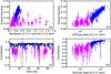 |
Fig. 11 Timing analysis performed for every time bin with length of at least of 200 s and S/N ≥ 25 in obs1 and obs2. The origin of times is the same as specified in Fig. 1. Panel a): pulsed fraction as a function of the HR. Panel b): pulsed fraction as a function of the source total intensity. Panel c): linear correlation coefficient between the average pulse profile and the pulse profile computed in each time bin (the shaded yellow area represents the expected range of correlation values at 1σ c.l. that all profiles should have if no changes occur other than the average one; the level of timing noise of the observation was also taken into account). Panel d): the correlation coefficient as function of the source count rate. The uncertainties are reported at 1σ c.l. and are computed for the pulsed fraction and correlation coefficient using a bootstrapping technique with 1000 realizations. |
When inspected as a function of the HR, both the spectra and the pulse profiles of the magenta states displayed a particularly intriguing change for HR > 0.70. A striking comparison is shown in Figs. 5 and 6. Correspondingly, a strong jump in phase of the overtone is also observed (Fig. 11). The spectrum extracted during the time intervals when HR > 0.70 could not be well described by a thermal plus a Comptonization component. We showed that a partially covering power-law model provided a significantly better fit to the data. The additional absorbing material implied by this model requires that part of the power-law emission from the source is seen through an absorption column density that is a factor of ~10 higher than the average value. We suggest below that the increased column density of the hard magenta states can be associated with the production of strong outflows during the switch from a weak to the strong propeller regime.
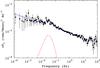 |
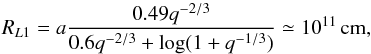
Fig. 12 Power spectral density observed during obs2. The power spectrum was rebinned geometrically using a factor of 1.30, and subtracted of a white noise level of 1.9948(5). The model used to fit the spectrum (red solid line) is the sum of a flicker noise component (Eq. (2)) and a Lorentzian (red dashed line). |
The definition of weak and strong propeller was introduced by Romanova et al. (2004) following the results of 2D and 3D
magnetohydrodynamic simulations of accreting AMXPs. If we estimate the position of the inner
boundary of the accretion disk around the NS with the usual equation (see, e.g. Frank et al. 2002)  (3)(here L36 is the X-ray
luminosity in units of 1036 erg/s and μ26 is the NS magnetic moment in units of
1026 G cm3), it is well-known that accretion onto the NS can proceed
unimpeded as long as this radius is smaller than the so-called corotation radius
(3)(here L36 is the X-ray
luminosity in units of 1036 erg/s and μ26 is the NS magnetic moment in units of
1026 G cm3), it is well-known that accretion onto the NS can proceed
unimpeded as long as this radius is smaller than the so-called corotation radius
 (4)Here P-3 is the NS spin period in units of 1 ms
and we assumed for both Rco and Rm an NS mass of
1 M⊙ and a radius of 10 km. The corotation
radius represents the distance from the NS at which the rotational velocity of the NS
magnetic field lines, anchored to the star, is higher than that of the material at the inner
boundary of the disk. When Rm approaches Rco, accretion is
partly inhibited by the fast rotation of the star and material at the inner boundary of the
disk tends to be ejected from the system instead of being accreted. In the weak propeller,
the magnetospheric radius is relatively close to the corotation radius (Rm ≃
Rco), and for typical parameters the
quantity of material that is accreted onto the star is comparable with the amount that is
ejected through outflows (see Figs. 14–16 in Ustyugova et
al. 2006). The latter can be in the form of winds emerging from the external layers
of the accretion disk or collimated in mildly relativistic jets. When Rm ≳
Rco, the system switches to the strong
propeller regime. In this regime, the amount of ejected material in the outflows can be as
high as 10 times the one that is effectively accreted onto the NS and up to ~70% of the total mass inflow rate along
the disk (see also Lii et al. 2012, 2014; Lovelace et al.
2013, and references therein). The material ejected from the system through the
outflows attains relativistic speeds and thus a number of different physical processes
(e.g., Fermi acceleration caused by shocks between the ejected material and
the surrounding medium, and inverse Compton scattering of low-energy photons by the bulk
motion of the outflow) are expected to contribute to the source X-ray emission and lead to a
harder spectrum than that produced by the accretion. A similar scenario was also invoked to
explain the hard spectra of the intermittent AMXP Aql X-1 during its transitions from
accretion to the propeller state (Zhang et al. 1998)
and in similar transitions observed in a number of accreting pulsars (see e.g., Cui 1997, and references therein). The presence of
outflows in IGR J18245–2452 due to possible strong propeller phases is also supported by the
detection of a very pronounced variability of the source in the radio domain (see
Appendix B and Pavan et al. 2013).
(4)Here P-3 is the NS spin period in units of 1 ms
and we assumed for both Rco and Rm an NS mass of
1 M⊙ and a radius of 10 km. The corotation
radius represents the distance from the NS at which the rotational velocity of the NS
magnetic field lines, anchored to the star, is higher than that of the material at the inner
boundary of the disk. When Rm approaches Rco, accretion is
partly inhibited by the fast rotation of the star and material at the inner boundary of the
disk tends to be ejected from the system instead of being accreted. In the weak propeller,
the magnetospheric radius is relatively close to the corotation radius (Rm ≃
Rco), and for typical parameters the
quantity of material that is accreted onto the star is comparable with the amount that is
ejected through outflows (see Figs. 14–16 in Ustyugova et
al. 2006). The latter can be in the form of winds emerging from the external layers
of the accretion disk or collimated in mildly relativistic jets. When Rm ≳
Rco, the system switches to the strong
propeller regime. In this regime, the amount of ejected material in the outflows can be as
high as 10 times the one that is effectively accreted onto the NS and up to ~70% of the total mass inflow rate along
the disk (see also Lii et al. 2012, 2014; Lovelace et al.
2013, and references therein). The material ejected from the system through the
outflows attains relativistic speeds and thus a number of different physical processes
(e.g., Fermi acceleration caused by shocks between the ejected material and
the surrounding medium, and inverse Compton scattering of low-energy photons by the bulk
motion of the outflow) are expected to contribute to the source X-ray emission and lead to a
harder spectrum than that produced by the accretion. A similar scenario was also invoked to
explain the hard spectra of the intermittent AMXP Aql X-1 during its transitions from
accretion to the propeller state (Zhang et al. 1998)
and in similar transitions observed in a number of accreting pulsars (see e.g., Cui 1997, and references therein). The presence of
outflows in IGR J18245–2452 due to possible strong propeller phases is also supported by the
detection of a very pronounced variability of the source in the radio domain (see
Appendix B and Pavan et al. 2013).
Assuming an average X-ray luminosity of 1035 erg/s for all the magenta states, the condition
Rm ≃
Rco for the onset of the weak propeller in
IGR J18245–2452 would imply a magnetic field for the NS in this system of ~3 × 10⁸ G, which is in the range
usually inferred for other AMXPs (see, e.g., Papitto et al.
2012, and references therein) and consistent with the value given previously in
Paper I. However, it is well-known that large uncertainties affect the estimates of the
magnetospheric radius given in Eq. (3), and
therefore the NS magnetic field inferred from this argument should be taken with caution
(see discussion in Bozzo et al. 2009). Limits on the
NS magnetic field can also be inferred from IGR J18245–2452’s radio pulsar nature. For the
NS to be active as a radio pulsar, the electrical voltage gap (formed by a dipolar magnetic
field that corotates with the NS) should extract charged particles from the NS surface,
accelerate them along the magnetic field lines, and eventually lead to a pair cascade that
is ultimately responsible for the observed coherent radio emission (Goldreich & Julian 1969; Ruderman
& Sutherland 1975). The so-called pulsar death line sets a theoretical limit
for this process to take place. In a purely central dipolar case, for the spin period of
IGR J18245–2452, this would lead to a lower limit of the magnetic field of B> 6.5 × 10⁷ G
(see Eq. (6) in Chen & Ruderman 1993)8. Furthermore, we note that the weakest magnetic field
ever measured for a radio pulsar is 6.7 ×
107 G for the binary millisecond pulsar PSR
J2229+2643 (spin period
2.9 ms; Camilo & Nice 1995; Wolszczan et al. 2000). An upper limit can be determined from the
pulsar’s spin-down rate during the rotationally-powered phase. However, we note that a
strong limitation to this measurement is provided by the motion in the cluster’s
gravitational field, which yields a spurious frequency derivative of ≈2
× 10-13 Hz/s, which is two orders of magnitude larger than the
frequency derivative usually observed from millisecond pulsars of the Galactic field. To
determine the value of the acceleration in the cluster potential, we followed the procedure
described by Papitto et al. (2012) using the pulsar’s
radio localisation (Pavan et al. 2013), the measured
cluster center coordinates (Becker et al. 2003), the
values of the M 28 core and tidal radii (Trager et al.
1995), and its total estimated mass of 5.5 × 10⁵ M⊙ (Boyles et al. 2011). Considering the source spin period,
and the upper limit on the period derivative from the cluster potential, we can derive an
upper limit on the NS surface dipolar magnetic field at the equator of
 G. We conclude that the magnetic field of
IGR J18245–2452 is constrained to be in the ~0.7–35 ×
108 G range, in line with what is predicted by its propeller
state.
G. We conclude that the magnetic field of
IGR J18245–2452 is constrained to be in the ~0.7–35 ×
108 G range, in line with what is predicted by its propeller
state.
Our analysis of the XMM-Newton data also revealed that the aperiodic
variability of IGR J18245–2452 is dominated by a flicker noise component extending to less
than fmin =
10-4 Hz, similarly to black-hole binaries in the soft states
(e.g., Churazov et al. 2001). This is at odds with
the low-frequency noise properties of other AMP (van
Straaten et al. 2005), which are usually described by a flat topped noise with a
characteristic frequency of ~0.1–1 Hz. The hour-long time-scale of the noise observed from
IGR J18245–2452 rules out that this variability is produced in the inner rings of the
accretion disk (where most of the X-rays come from) because the dynamical and viscous
time-scales are much shorter there. Lyubarskii (1997)
interpreted the flicker noise observed from accreting compact objects in terms of variations
of the accretion rate at different radii, each characterized by a different viscous
time-scale. These fluctuations propagate to the inner parts of the disk, generating the
observed X-ray variability. According to this model, the longest time-scales are introduced
in the outer parts of the disk, the radius of which is related to the low-frequency break
observed in the power spectrum by  (5)where α is the disk viscosity
parameter of a Shakura-Sunyaev disk. This size is smaller by a factor ~2 than the size of the NS Roche lobe:
(5)where α is the disk viscosity
parameter of a Shakura-Sunyaev disk. This size is smaller by a factor ~2 than the size of the NS Roche lobe:
 (6)where a = 2 ×
1011(Mt/ 1.6
M⊙)1 / 3 cm is the orbital
separation between the two stars, Mt is the total mass of the system,
q =
M2/M1 is the
binary mass ratio, and values of M2 = 0.2 M⊙ and
M1 =
1.4 M⊙ were considered for the donor and the
NS mass, respectively (see Paper I). In black-hole binaries, the rms variability is more
pronounced at high energy (≳6 keV), suggesting that an extended optically thin corona around the
accretion disk causes the X-ray variability. In our case, there is no significant energy
dependency of the shape of the PDS, while coherent timing reveals a relatively high and
constant pulsed fraction above 4 keV. This supports the idea that the X-rays recorded from
IGR J18245–2452 are produced by the accretion stream close to the NS, as discussed earlier
in this section.
(6)where a = 2 ×
1011(Mt/ 1.6
M⊙)1 / 3 cm is the orbital
separation between the two stars, Mt is the total mass of the system,
q =
M2/M1 is the
binary mass ratio, and values of M2 = 0.2 M⊙ and
M1 =
1.4 M⊙ were considered for the donor and the
NS mass, respectively (see Paper I). In black-hole binaries, the rms variability is more
pronounced at high energy (≳6 keV), suggesting that an extended optically thin corona around the
accretion disk causes the X-ray variability. In our case, there is no significant energy
dependency of the shape of the PDS, while coherent timing reveals a relatively high and
constant pulsed fraction above 4 keV. This supports the idea that the X-rays recorded from
IGR J18245–2452 are produced by the accretion stream close to the NS, as discussed earlier
in this section.
According to our interpretation, the peculiar behavior of IGR J18245–2452 in the X-ray domain is mainly due to switches between accretion to weak and strong propeller states. This requires the magnetospheric radius to be close to the coronation radius across the entire outburst. A similar situation has previously been investigated in several theoretical studies (Spruit & Taam 1993; Rappaport et al. 2004; D’Angelo & Spruit 2010, 2012) and applied to interpret observations of a number of AMXP in outbursts. For SAX J1808.4–3658 and NGC 6440 X-2 the switch between accretion and propeller was used to interpret periods of intense quasi-periodic flaring activity (Patruno et al. 2009; Patruno & D’Angelo 2013). Evidence that the magnetospheric and co-rotation radii remain locked in outburst was also reported for XTE J1814–338 (Haskell & Patruno 2011). Patruno et al. (2012) proposed later that such locking might indeed occur during most of the AMXP outbursts.
However, IGR J18245–2452 displayed a different kind of X-ray variability than that reported here. This was revealed during the analysis of a faint outburst from the source discovered serendipitously in Chandra archival data from 2002. During this event, IGR J18245–2452 reached a luminosity of ~1033 erg/s and its X-ray variability was ascribed to the locking of the magnetospheric radius in the proximity of the source light-cylinder (Linares et al. 2014). The same scenario was used later to interpret a period of pronounced low-luminosity X-ray variability observed from PSR J1023+0038. On this occasion the radio pulsations from the source disappeared and its GeV emission increased by a factor of ~5 (possibly because of outflows and the formation of shocks in the intra-binary environment; Takata et al. 2014; Patruno et al. 2014). A similar behavior was also observed from the source XSS J12270–289 (Papitto et al. 2014; Bassa et al. 2014; Roy & Bhattacharya 2014). Millisecond pulsars in binary systems thus seem to display frequent episodes of mass accretion during which the magnetospheric boundary can either be locked at the light cylinder or at the co-rotation radius. In the former case, accretion is strongly inhibited and the system is observed as a relatively faint X-ray emitter (LX ~ 1032 − 33 erg/s); in the latter, case canonical outbursts might occur and peak X-ray luminosities of LX ~ 1035 − 36 erg/s can be achieved.
5. Conclusions
We analyzed the peculiar variability showed in the X-ray domain by the swinging pulsar IGR J18245–2452. We discussed that the results obtained from the spectroscopic and the timing analysis of the XMM-Newton data could be reasonably well described by assuming an unstable accretion phase in which the material from the disk does not always reach the NS surface quietly, but proceeds in a hiccup fashion: accretion is strongly inhibited for a substantial fraction of time by the stellar rotation that causes the onset of a propeller regime. This might produce strong outflows that generate a strongly variable GHz emission and lead to the sporadic appearance of a completely different X-ray spectrum than that of the remaining accretion phases.
Observations of possible future outbursts from IGR J18245–2452 with the next generation of X-ray timing experiments (e.g., LOFT; Feroci et al. 2012) will enable us to perform timing and spectral analyses with higher statistics down to very short time-scales, providing crucial insights into the mechanisms responsible for the peculiar X-ray variability of this source and other AMXPs.
Note, however, that when different configurations of the magnetic field (i.e. twisted field lines) are considered, this field limit can decrease by about an order of magnitude (~5 × 10⁶ G; see Eq. (9) in Chen & Ruderman 1993).
We used the ISIS software package (version 1.6.2–16) for the spectral analysis presented in this section.
Acknowledgments
The authors thank the XMM-Newton, Swift, and ATCA PIs and the respective shift teams for their availability in quickly performing the target of opportunity observations used in this work. This work made use of data supplied by the UK Swift Science Data Centre at the University of Leicester. A.P. and N.R. acknowledge grants AYA2012-39303 and SGR2009- 811. A.P. is supported by a Juan de la Cierva fellowship. N.R. is supported by a Ramon y Cajal fellowship and by an NWO Vidi Award. We thank our colleagues M. Audard, M. Guainazzi, E. Kuulkers, S. E. Motta, A. Patruno, and A. Tramacere, for contributing with stimulating discussions and advices.
References
- Alpar, M. A., Cheng, A. F., Ruderman, M. A., & Shaham, J. 1982, Nature, 300, 728 [NASA ADS] [CrossRef] [Google Scholar]
- Archibald, A. M., Stairs, I. H., Ransom, S. M., et al. 2009, Science, 324, 1411 [NASA ADS] [CrossRef] [PubMed] [Google Scholar]
- Bassa, C. G., Patruno, A., Hessels, J. W. T., et al. 2014, MNRAS, 441, 1825 [Google Scholar]
- Becker, W., Swartz, D. A., Pavlov, G. G., et al. 2003, ApJ, 594, 798 [NASA ADS] [CrossRef] [Google Scholar]
- Beloborodov, A. M. 2002, ApJ, 566, L85 [NASA ADS] [CrossRef] [Google Scholar]
- Boyles, J., Lorimer, D. R., Turk, P. J., et al. 2011, ApJ, 742, 51 [NASA ADS] [CrossRef] [Google Scholar]
- Bozzo, E., Stella, L., Vietri, M., & Ghosh, P. 2009, A&A, 493, 809 [NASA ADS] [CrossRef] [EDP Sciences] [Google Scholar]
- Bozzo, E., Giunta, A., Cusumano, G., et al. 2011, A&A, 531, A130 [NASA ADS] [CrossRef] [EDP Sciences] [Google Scholar]
- Bozzo, E., Romano, P., Ferrigno, C., et al. 2013, A&A, 556, A30 [NASA ADS] [CrossRef] [EDP Sciences] [Google Scholar]
- Burderi, L., Di Salvo, T., D’Antona, F., Robba, N. R., & Testa, V. 2003, A&A, 404, L43 [NASA ADS] [CrossRef] [EDP Sciences] [Google Scholar]
- Burrows, D. N., Hill, J. E., Nousek, J. A., et al. 2005, Space Sci. Rev., 120, 165 [NASA ADS] [CrossRef] [Google Scholar]
- Camilo, F., & Nice, D. J. 1995, ApJ, 445, 756 [NASA ADS] [CrossRef] [Google Scholar]
- Campana, S., Colpi, M., Mereghetti, S., Stella, L., & Tavani, M. 1998, A&ARv, 8, 279 [NASA ADS] [CrossRef] [Google Scholar]
- Chen, K., & Ruderman, M. 1993, ApJ, 402, 264 [NASA ADS] [CrossRef] [Google Scholar]
- Churazov, E., Gilfanov, M., & Revnivtsev, M. 2001, MNRAS, 321, 759 [NASA ADS] [CrossRef] [Google Scholar]
- Cui, W. 1997, ApJ, 482, L163 [NASA ADS] [CrossRef] [Google Scholar]
- D’Angelo, C. R., & Spruit, H. C. 2010, MNRAS, 406, 1208 [NASA ADS] [Google Scholar]
- D’Angelo, C. R., & Spruit, H. C. 2012, MNRAS, 420, 416 [NASA ADS] [CrossRef] [Google Scholar]
- Eckert, D., Del Santo, M., Bazzano, A., et al. 2013, ATel, 4925 [Google Scholar]
- Evans, P. A., Beardmore, A. P., Page, K. L., et al. 2009, MNRAS, 397, 1177 [NASA ADS] [CrossRef] [Google Scholar]
- Falanga, M., Kuiper, L., Poutanen, J., et al. 2005, A&A, 444, 15 [NASA ADS] [CrossRef] [EDP Sciences] [Google Scholar]
- Feroci, M., Stella, L., van der Klis, M., et al. 2012, Exp. Astron., 34, 415 [NASA ADS] [CrossRef] [Google Scholar]
- Frank, J., King, A., & Raine, D. J. 2002, Accretion Power in Astrophysics: 3rd edn. (Cambridge: Cambridge University Press) [Google Scholar]
- Garmire, G. P., Bautz, M. W., Ford, P. G., Nousek, J. A., & Ricker, Jr., G. R. 2003, in SPIE Conf. Ser. 4851, eds. J. E. Truemper, & H. D. Tananbaum, 28 [Google Scholar]
- Gehrels, N. 1986, ApJ, 303, 336 [NASA ADS] [CrossRef] [Google Scholar]
- Gierliński, M., & Poutanen, J. 2005, MNRAS, 359, 1261 [NASA ADS] [CrossRef] [Google Scholar]
- Gierliński, M., Zdziarski, A. A., Poutanen, J., et al. 1999, MNRAS, 309, 496 [NASA ADS] [CrossRef] [Google Scholar]
- Gierliński, M., Done, C., & Barret, D. 2002, MNRAS, 331, 141 [NASA ADS] [CrossRef] [Google Scholar]
- Gilfanov, M., Revnivtsev, M., Sunyaev, R., & Churazov, E. 1998, A&A, 338, L83 [NASA ADS] [Google Scholar]
- Goldreich, P., & Julian, W. H. 1969, ApJ, 157, 869 [NASA ADS] [CrossRef] [Google Scholar]
- Gooch, R. 1996, in ASP Conf. Ser., 101, Astronomical Data Analysis Software and Systems V, eds. G. H. Jacoby, & J. Barnes, 80 [Google Scholar]
- Haskell, B., & Patruno, A. 2011, ApJ, 738, L14 [NASA ADS] [CrossRef] [Google Scholar]
- Ibragimov, A., & Poutanen, J. 2009, MNRAS, 400, 492 [NASA ADS] [CrossRef] [Google Scholar]
- Ibragimov, A., Kajava, J. J. E., & Poutanen, J. 2011, MNRAS, 415, 1864 [NASA ADS] [CrossRef] [Google Scholar]
- Illarionov, A. F., & Sunyaev, R. A. 1975, A&A, 39, 185 [NASA ADS] [Google Scholar]
- Jimenez-Garate, M. A., Hailey, C. J., den Herder, J. W., Zane, S., & Ramsay, G. 2002, ApJ, 578, 391 [NASA ADS] [CrossRef] [Google Scholar]
- Jimenez-Garate, M. A., Raymond, J. C., Liedahl, D. A., & Hailey, C. J. 2005, ApJ, 625, 931 [NASA ADS] [CrossRef] [Google Scholar]
- Kaastra, J. S., de Vries, C. P., Costantini, E., & den Herder, J. W. A. 2009, A&A, 497, 291 [NASA ADS] [CrossRef] [EDP Sciences] [Google Scholar]
- Kajava, J. J. E., Ibragimov, A., Annala, M., Patruno, A., & Poutanen, J. 2011, MNRAS, 417, 1454 [NASA ADS] [CrossRef] [Google Scholar]
- Lamb, F. K., Boutloukos, S., Van Wassenhove, S., et al. 2009, ApJ, 706, 417 [NASA ADS] [CrossRef] [Google Scholar]
- Lebrun, F., Leray, J. P., Lavocat, P., et al. 2003, A&A, 411, L141 [NASA ADS] [CrossRef] [EDP Sciences] [Google Scholar]
- Lii, P., Romanova, M., & Lovelace, R. 2012, MNRAS, 420, 2020 [NASA ADS] [CrossRef] [Google Scholar]
- Lii, P. S., Romanova, M. M., Ustyugova, G. V., Koldoba, A. V., & Lovelace, R. V. E. 2014, MNRAS, 441, 86 [NASA ADS] [CrossRef] [Google Scholar]
- Linares, M. 2013, ATel, 4960 [Google Scholar]
- Linares, M., Bahramian, A., Heinke, C., et al. 2014, MNRAS, 438, 251 [NASA ADS] [CrossRef] [Google Scholar]
- Lovelace, R. V. E., Romanova, M. M., & Lii, P. 2013 [arXiv:1306.1160] [Google Scholar]
- Lyubarskii, Y. É. 1997, MNRAS, 292, 679 [NASA ADS] [CrossRef] [Google Scholar]
- Merloni, A., Fabian, A. C., & Ross, R. R. 2000, MNRAS, 313, 193 [NASA ADS] [CrossRef] [Google Scholar]
- Migliari, S., & Fender, R. P. 2006, MNRAS, 366, 79 [NASA ADS] [CrossRef] [Google Scholar]
- Pallanca, C., Dalessandro, E., Ferraro, F. R., Lanzoni, B., & Beccari, G. 2013, ApJ, 773, 122 [NASA ADS] [CrossRef] [Google Scholar]
- Papitto, A., Riggio, A., di Salvo, T., et al. 2010, MNRAS, 407, 2575 [NASA ADS] [CrossRef] [Google Scholar]
- Papitto, A., Di Salvo, T., Burderi, L., et al. 2012, MNRAS, 423, 1178 [NASA ADS] [CrossRef] [Google Scholar]
- Papitto, A., Bozzo, E., Ferrigno, C., et al. 2013a, ATel, 4959 [Google Scholar]
- Papitto, A., Ferrigno, C., Bozzo, E., et al. 2013b, Nature, 501, 517 [NASA ADS] [CrossRef] [PubMed] [Google Scholar]
- Papitto, A., Torres, D. F., & Li, J. 2014, MNRAS, 438, 2105 [NASA ADS] [CrossRef] [Google Scholar]
- Patruno, A., & D’Angelo, C. 2013, ApJ, 771, 94 [NASA ADS] [CrossRef] [Google Scholar]
- Patruno, A., & Watts, A. L. 2012 [arXiv:1206.2727] [Google Scholar]
- Patruno, A., Watts, A., Klein Wolt, M., Wijnands, R., & van der Klis, M. 2009, ApJ, 707, 1296 [NASA ADS] [CrossRef] [Google Scholar]
- Patruno, A., Haskell, B., & D’Angelo, C. 2012, ApJ, 746, 9 [NASA ADS] [CrossRef] [Google Scholar]
- Patruno, A., Archibald, A. M., Hessels, J. W. T., et al. 2014, ApJ, 781, L3 [NASA ADS] [CrossRef] [Google Scholar]
- Pavan, L., Wong, G., Wieringa, M. H., et al. 2013, ATel, 4981 [Google Scholar]
- Porquet, D., & Dubau, J. 2000, A&AS, 143, 495 [NASA ADS] [CrossRef] [EDP Sciences] [Google Scholar]
- Porquet, D., Mewe, R., Dubau, J., Raassen, A. J. J., & Kaastra, J. S. 2001, A&A, 376, 1113 [NASA ADS] [CrossRef] [EDP Sciences] [Google Scholar]
- Poutanen, J. 2006, Adv. Space Res., 38, 2697 [NASA ADS] [CrossRef] [Google Scholar]
- Radhakrishnan, V., & Srinivasan, G. 1982, Current Science, 51, 1096 [Google Scholar]
- Rappaport, S. A., Fregeau, J. M., & Spruit, H. 2004, ApJ, 606, 436 [NASA ADS] [CrossRef] [Google Scholar]
- Riggio, A., Papitto, A., Burderi, L., & di Salvo, T. 2011, in AIP Conf. Ser. 1357, eds. M. Burgay, N. D’Amico, P. Esposito, A. Pellizzoni, & A. Possenti, 151 [Google Scholar]
- Romano, P., Cusumano, G., Campana, S., et al. 2005, in SPIE Conf. Ser. 5898, ed. O. H. W. Siegmund, 357 [Google Scholar]
- Romano, P., Moretti, A., Banat, P. L., et al. 2006, A&A, 450, 59 [NASA ADS] [CrossRef] [EDP Sciences] [Google Scholar]
- Romanova, M. M., Ustyugova, G. V., Koldoba, A. V., & Lovelace, R. V. E. 2004, ApJ, 616, L151 [NASA ADS] [CrossRef] [Google Scholar]
- Roy, J., & Bhattacharya, B. 2014, ATel, 5890 [Google Scholar]
- Ruderman, M. A., & Sutherland, P. G. 1975, ApJ, 196, 51 [NASA ADS] [CrossRef] [EDP Sciences] [Google Scholar]
- Sault, R. J., Teuben, P. J., & Wright, M. C. H. 1995, in Astronomical Data Analysis Software and Systems IV, eds. R. A. Shaw, H. E. Payne, & J. J. E. Hayes, AIP Conf. Ser., 77, 433 [Google Scholar]
- Seaquist, E. R. 1993, Rep. Prog. Phys., 56, 1145 [NASA ADS] [CrossRef] [Google Scholar]
- Serino, M., Takagi, T., Negoro, H., et al. 2013, ATel, 4961 [Google Scholar]
- Spruit, H. C., & Taam, R. E. 1993, ApJ, 402, 593 [CrossRef] [Google Scholar]
- Takata, J., Li, K. L., Leung, G. C. K., et al. 2014, ApJ, 785, 131 [NASA ADS] [CrossRef] [Google Scholar]
- Trager, S. C., King, I. R., & Djorgovski, S. 1995, AJ, 109, 218 [NASA ADS] [CrossRef] [Google Scholar]
- Ubertini, P., Lebrun, F., Di Cocco, G., et al. 2003, A&A, 411, L131 [NASA ADS] [CrossRef] [EDP Sciences] [Google Scholar]
- Ustyugova, G. V., Koldoba, A. V., Romanova, M. M., & Lovelace, R. V. E. 2006, ApJ, 646, 304 [NASA ADS] [CrossRef] [Google Scholar]
- van Straaten, S., van der Klis, M., & Wijnands, R. 2005, ApJ, 619, 455 [NASA ADS] [CrossRef] [Google Scholar]
- Wilms, J., Reynolds, C. S., Begelman, M. C., et al. 2001, MNRAS, 328, L27 [NASA ADS] [CrossRef] [Google Scholar]
- Wilson, W. E., Ferris, R. H., Axtens, P., et al. 2011, MNRAS, 416, 832 [NASA ADS] [CrossRef] [Google Scholar]
- Wolszczan, A., Doroshenko, O., Konacki, M., et al. 2000, ApJ, 528, 907 [NASA ADS] [CrossRef] [Google Scholar]
- Zhang, S. N., Yu, W., & Zhang, W. 1998, ApJ, 494, L71 [NASA ADS] [CrossRef] [Google Scholar]
Appendix A: Analysis of the full-resolution RGS spectra
Best-fit model parameters of O vii lines during obs2.
During the analysis of the full-resolution RGS spectra of IGR J18245–2452 in obs2 (which have a much longer exposure time than obs1, see Table 1), we noticed a convincing hint of emission lines from O vii around 22 Å. Because these lines do not affect our discussion and conclusion about the source spectral and timing variability reported in Sects. 4 and 5, we summarize this result here.
Figure A.1 shows the RGS2 spectrum in obs2 after rebinning to achieve a minimum S/N of 3.0 in each wavelength bin)9. Table A.1 gives the best determined parameters obtained by fitting the two RGS spectra in obs2 with a model comprising the continuum determined in the broad-band analysis (Sect. 3.1) plus two narrow Gaussian lines (we used the χ2 statistics with weights according to Gehrels 1986). The wavelengths of the two emission lines were well constrained, while only an upper limit was obtained on their width. No forbidden line (22.10 Å) or lines typical of other isotopes (C v, N vi, Ne x, Mg xi, and Si xii) were significantly detected.
The two emission lines correspond to the oxygen triplet. The intercombination line is at the expected wavelength (the upper limit on its Doppler broadening is about 700 km s-1), while the resonance line appears to be slightly redshifted and the upper limit on its width is larger. The absence of a forbidden line can either be due to the high density of the gas (Ne ≳ 1011 cm-3) or to the presence of an intense UV field in the line forming region (Porquet & Dubau 2000; Porquet et al. 2001), as expected in the proximity of the X-ray irradiated companion star (Pallanca et al. 2013). If we assume that the lines can be broadened by the plasma orbital motion, the upper limit on the width of the intercombination line is compatible with the Keplerian velocity at the orbital separation of the system, while the slightly broader resonance line would favor emission from an inner region of the disk. This constraint is not stringent, however, as it was suggested that emission lines that originate in the outer layers of an accretion disk might be narrower than naively expected (Jimenez-Garate et al. 2002, 2005). We remark that the relatively low statistics of the RGS spectrum do not allow us to perform an orbital phase-resolved analysis of the oxygen lines.
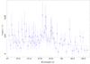 |
Fig. A.1 Zoom of the RGS2 spectrum of obs2 rebinned to achieve an S/N of 3 in each bin around the O vii triplet. The width of lines is fixed to zero. |
Appendix B: Analysis of the ATCA observation of IGR J18245–2452
In this appendix, we report on the analysis of the radio observation performed in the direction of IGR J18245–2452 by the Australia Telescope Compact Array (ATCA; Target of Opportunity project CX258) for ~6 h on 2013 April 5. The preliminary results of this observation were reported by Pavan et al. (2013) and are summarized in Paper I, but the data analysis was not presented in full detail yet.
 |
Fig. B.1 ATCA lightcurve of IGR J18245–2452 in the two frequencies (5.5 GHz, panel a), and 9 GHz, panel b)) and the calculated spectral index α, panel c). We also reported in the upper panel the 0.5–10 keV lightcurve from the Swift/XRT observation ID. 00032785003 (in blue). These were the only X-ray data collected quasi-simultaneously with the ATCA observation. |
The data considered here were collected with the new Compact Array Broadband Backend (CABB, Wilson et al. 2011) in the hybrid array configuration H214 at wavelengths of 6 and 3 cm (ν = 5.5 and 9 GHz). The observation was carried out in dual-frequency mode, with ~3.7 hours of integration time, split into two periods separated by approximately 2.5 h. The primary calibrator was PKS B1934–638, while PKS 1817–254 was used for phase calibration. The data were analysed with the miriad (Sault et al. 1995) and karma (Gooch 1996) software packages distributed by ATNF.
Radio images of the observation were created using the miriad multifrequency synthesis and robust weighting (Sault et al. 1995). They were deconvolved using the mfclean and restor algorithms with primary-beam correction applied using the linmos task. A similar procedure was used for the U and Q Stokes parameter maps.
A single compact source was detected in our images within the M28 globular cluster (the image resolution was 4.8′′ × 1.0′′ at PA = 9 deg with an estimated rms noise of 11 μJy/beam at 5.5GHz and 3.0′′ × 0.64′′ at PA = 10 deg; with an estimated rms noise of 12 μJy/beam at 9 GHz). Its position coincides well with the X-ray counterpart of PSR J18245-2452 (Paper I). The measured flux density of the source was (0.62 ± 0.03) mJy at 5.5 GHz and (0.75 ± 0.04) mJy at 9 GHz (Pavan et al. 2013). The radio emission recorded from IGR J18245–2452 therefore has an intensity similar to that of other AMXPs in outburst (Migliari & Fender 2006; Patruno & Watts 2012).
We extracted radio light curves of the source at the two observing frequencies by using the miriad/uvplt task, and averaging the data at temporal intervals of 2 min. The source showed variations of intensity during the first part of the observation, reaching up to 2 mJy, while during the second part, the mean flux density was not significantly variable (Fig. B.1). To better study the observed radio variability, we estimated the variation of source spectral index α with time. The lightcurves and spectral index are shown in Fig. B.1. The spectral index varies significantly in the range −0.2–0.8 and has a mean value of α ~ + 0.39 ± 0.21 (where α = [log (Fν1/Fν2)] / [log (ν1 /ν2)], ν1 = 9 GHz, and ν2 = 5.5 GHz). Splitting the two observational bands into bins of bandwidth 128 MHz allowed us to obtain a refined mean value of the spectral index α = + 0.39 ± 0.06. This inverted radio spectrum indicates the IGR J18245–2452 has an optically thick synchrotron-emitting region or a mixture of thermal and synchrotron emission, typical of a persistent jet or a less collimated outflow (e.g., Seaquist 1993).
We report in Fig. B.1 the only available
quasi-simultaneous X-ray observation of the source. These data (observation
ID. 00032785003) were collected with the Swift/XRT on 2013 April 5 from
16:58:06 to 19:04:26 (UTC) and analyzed with the Leicester XRT on-line tool10 (Evans et al.
2009). The observation is divided into two snapshots that occur before the start
of the radio data and at the end of the second radio flare. The spectra of the two
snapshots were extracted separately and then fit together with an absorbed power-law
model. The first snapshot was affected by pile-up and thus the corresponding spectrum was
extracted by using an annular region with inner radius of 4 pixels and external radius of
20 pixels, in agreement with standard procedures (Burrows
et al. 2005; Romano et al. 2006). The
photon indices of the power laws were left free to vary in the fits, while the absorption
column density was constrained to be the same for the two spectra. The best-fit model
( , 32 d.o.f.) gave an absorption column
density of NH =
(4.1 ± 1.6) × 1021 cm-2 and photon indices of
(1.45 ± 0.25) and
(1.8 ± 0.3), for the two
snapshots. The corresponding fluxes (0.5–10 keV) were (6.4 ± 0.8) and (4.3 ± 0.6) × 10-11 erg / s /
cm2. We note that the spectral properties and fluxes of the
two XRT snapshots performed simultaneously with the ATCA observation are similar to those
measured during the soft magenta states identified by XMM (see Table 5). The slightly
steeper power-law index of the second snapshot might be generated by black-body emission,
which went undetected owing to the limited number of collected photons. These results
support the idea that outflows might be produced during the magenta states of
IGR J18245–2452.
, 32 d.o.f.) gave an absorption column
density of NH =
(4.1 ± 1.6) × 1021 cm-2 and photon indices of
(1.45 ± 0.25) and
(1.8 ± 0.3), for the two
snapshots. The corresponding fluxes (0.5–10 keV) were (6.4 ± 0.8) and (4.3 ± 0.6) × 10-11 erg / s /
cm2. We note that the spectral properties and fluxes of the
two XRT snapshots performed simultaneously with the ATCA observation are similar to those
measured during the soft magenta states identified by XMM (see Table 5). The slightly
steeper power-law index of the second snapshot might be generated by black-body emission,
which went undetected owing to the limited number of collected photons. These results
support the idea that outflows might be produced during the magenta states of
IGR J18245–2452.
All Tables
Results of the fits to the average spectra extracted by using all the available exposure time in obs1 and obs2.
Spectral parameters of the best-fit models to the rate-resolved spectra of IGR J18245–2452 during the blue states.
Reduced χ2 and degrees of freedom of various models for hardness-resolved spectra.
Parameters of the best-fit models to the HR-resolved spectra of the magenta using the nthComp plus black-body.
Best-fit model parameters of the power spectra density extracted by using the entire exposure time available in obs1 and obs2.
All Figures
|
Fig. 1 Top panel: XMM-Newton lightcurve of IGR J18245–2452 extracted from obs1 and obs2 in the 0.5–3.5 keV energy band. The vertical dashed line represents the separation between the two observations. Times of obs1 are measured starting from 00:25:22 on 2013 April 04 (TBD). For the second observation the start time is 2013 April 13 at 07:03:06 (TBD; note that times have been shifted by 26.3 ks for plotting purposes). Middle panel: same as before, but in the 3.5–11 keV energy range. This lightcurve was adaptively rebinned to achieve a signal-to-noise (S/N) ratio of 25 in each time bin, while the minimum bins size was set to 200 s (the same binning has been used for the lightcurve in the soft energy band). Bottom panel: hardness ratio (HR) calculated as the ratio of the hard and soft lightcurves. We plot with magenta symbols the time intervals in which the source count rate was lower than 30 cts/s, all the others are given in blue. The points with HR > 0.7 are highlighted with an open circle. |
| In the text | |
|
Fig. 2 Histogram of the count-rate derived from the combined lightcurves of the two observations (energy range 0.5–11 keV, time bin 1 s). The black solid line represents the total source count-rate. The black dashed line is the sum of two best-fit log-normal distributions, plotted in blue and magenta. |
| In the text | |
|
Fig. 3 Hardness-intensity diagram built by using all data in obs1 and obs2, which are displayed in Fig. 1 (time bin of 200 s). The black solid line separates the different intensity states: the points represented in magenta and blue have a count rate lower and higher than 30 cts/s, respectively. |
| In the text | |
|
Fig. 4 Average unfolded spectra of IGR J18245–2452 in obs1 and obs2. Colors refer to the different observations and instruments (red: EPIC-pn obs1; black: EPIC-pn obs2; green: RGS1 obs2; blue: RGS2 obs2; light blue: RGS1 obs1; magenta: RGS2 obs1). The best-fit model is reported in Table 2. We show in the lower panel the residuals from the best fit (see text for details). |
| In the text | |
|
Fig. 5 IGR J18245–2452 unfolded spectrum of the soft magenta state (HR < 0.25). The best-fit model (see Table 5) and the residuals from this fit are shown as well. Colors refer to the different observations and instruments (black: EPIC-pn obs1; red: EPIC-pn obs2; green: RGS obs1; blue: RGS obs2). |
| In the text | |
|
Fig. 6 IGR J18245–2452 unfolded spectrum of the hard magenta state (HR > 0.7). The best-fit model (see Table 5) and the residuals from this fit are shown as well. Colors refer to the different observations and instruments (black: EPIC-pn obs1; red: EPIC-pn obs2; green: RGS obs1; blue: RGS obs2). |
| In the text | |
|
Fig. 7 Pulse profiles of the combined obs1 and obs2 extracted during the different count-rate intervals of the blue states as in Table 3. In all panels of this figure, count rates were normalised to the maximum. Pulses are repeated twice for clarity and the red solid lines represent the best fits to the profiles with two sinusoidal functions as described in the text. The insets in each panel show the lightcurves of the two observations in the 0.5–11 keV energy range (as in Fig. 1) with the time intervals used to extract the pulse profiles highlighted in red. |
| In the text | |
|
Fig. 8 Parameters of the Fourier decomposition of the pulse profiles as a function of the source count-rate in the EPIC-pn data. The different parameters are defined in Eq. (1). Uncertainties are obtained by fitting Eq. (1) to the pulse profiles and given at 1σ c.l. |
| In the text | |
|
Fig. 9 Same as Fig. 7, but here the pulse profiles are extracted for different ranges of the source HR in the magenta states. |
| In the text | |
|
Fig. 10 Same as Fig. 8, but for the HR-resolved pulse profiles extracted in the magenta states (Fig. 9). Uncertainties are obtained by fitting Eq. (1) to the pulse profiles and given at 1σ c.l. |
| In the text | |
|
Fig. 11 Timing analysis performed for every time bin with length of at least of 200 s and S/N ≥ 25 in obs1 and obs2. The origin of times is the same as specified in Fig. 1. Panel a): pulsed fraction as a function of the HR. Panel b): pulsed fraction as a function of the source total intensity. Panel c): linear correlation coefficient between the average pulse profile and the pulse profile computed in each time bin (the shaded yellow area represents the expected range of correlation values at 1σ c.l. that all profiles should have if no changes occur other than the average one; the level of timing noise of the observation was also taken into account). Panel d): the correlation coefficient as function of the source count rate. The uncertainties are reported at 1σ c.l. and are computed for the pulsed fraction and correlation coefficient using a bootstrapping technique with 1000 realizations. |
| In the text | |
|
Fig. 12 Power spectral density observed during obs2. The power spectrum was rebinned geometrically using a factor of 1.30, and subtracted of a white noise level of 1.9948(5). The model used to fit the spectrum (red solid line) is the sum of a flicker noise component (Eq. (2)) and a Lorentzian (red dashed line). |
| In the text | |
|
Fig. A.1 Zoom of the RGS2 spectrum of obs2 rebinned to achieve an S/N of 3 in each bin around the O vii triplet. The width of lines is fixed to zero. |
| In the text | |
|
Fig. B.1 ATCA lightcurve of IGR J18245–2452 in the two frequencies (5.5 GHz, panel a), and 9 GHz, panel b)) and the calculated spectral index α, panel c). We also reported in the upper panel the 0.5–10 keV lightcurve from the Swift/XRT observation ID. 00032785003 (in blue). These were the only X-ray data collected quasi-simultaneously with the ATCA observation. |
| In the text | |
Current usage metrics show cumulative count of Article Views (full-text article views including HTML views, PDF and ePub downloads, according to the available data) and Abstracts Views on Vision4Press platform.
Data correspond to usage on the plateform after 2015. The current usage metrics is available 48-96 hours after online publication and is updated daily on week days.
Initial download of the metrics may take a while.