| Issue |
A&A
Volume 566, June 2014
|
|
|---|---|---|
| Article Number | A149 | |
| Number of page(s) | 13 | |
| Section | Cosmology (including clusters of galaxies) | |
| DOI | https://doi.org/10.1051/0004-6361/201322447 | |
| Published online | 26 June 2014 | |
Mass profile and dynamical status of the z ~ 0.8 galaxy cluster LCDCS 0504⋆
1 Astrophysics and Cosmology Research Unit, University of KwaZulu-Natal, Durban 4041, South Africa
e-mail: guennou@ukzn.ac.za
2 Aix-Marseille Université, CNRS, LAM (Laboratoire d’Astrophysique de Marseille) UMR 7326, 13388 Marseille, France
3 INAF/Osservatorio Astronomico di Trieste, via Tiepolo 11, 34143 Trieste, Italy
4 Institut d’Astrophysique de Paris (UMR 7095: CNRS & UPMC), 98bis Bd Arago, 75014 Paris, France
5 Departamento de Astronomia, Instituto de Astronomia Geofìsica e Ciências Atmosfèricas, Universidade de São Paulo, Rua do Matão 1226, 05508-900 São Paulo, Brazil
6 Department Physics & Astronomy & Center for Interdisciplinary Exploration and Research in Astrophysics (CIERA), Northwestern University, Evanston, IL 60208-2900, USA
7 Department of Physics and Astronomy, Ohio University, 251B Clippinger Lab, Athens, OH 45701, USA
8 Fermi National Accelerator Laboratory, PO Box 500, Batavia, IL 60510, USA
9 CSC/STSCi, 3700 San Martin Dr., Baltimore, MD 21218, USA
10 OCA, Cassiopée, Boulevard de l’Observatoire, BP 4229, 06304 Nice Cedex 4, France
11 INAF/Osservatorio Astronomico di Bologna, via Ranzani 1, 40127 Bologna, Italy
12 23 rue d’Yerres, 91230 Montgeron, France
13 Steward Observatory, University of Arizona, 933 N. Cherry Ave. Tucson, AZ 85721, USA
14 Department of Astronomy & Astrophysics, University of Toronto, 50 St George Street Toronto, Ontario M5S 3H4, Canada
15 Instituto de Astrofísica de Andalucía (CSIC), Glorieta de la Astronomía s/n, 18008 Granada, Spain
16 Kavli Institute for Particle Astrophysics and Cosmology, Stanford University, 2575 Sand Hill Rd., Menlo Park, CA 94025, USA
17 Laboratório de Astrofísica Teórica e Observacional, Universidade Estadual de Santa Cruz, Ilhéus, Brazil
18 Gemini Observatory, Casilla 603 La Serena, Chile
19 Argelander-Institut für Astronomie, Universitët Bonn, Auf dem Hügel 71, 53121 Bonn, Germany
20 Physics Department, University of California, Santa Barbara, CA 93601, USA
21 University of Vienna, Department of Astrophysics, Türkenschanzstr. 17, 1180 Wien, Austria
Received: 5 August 2013
Accepted: 16 March 2014
Context. Constraints on the mass distribution in high-redshift clusters of galaxies are currently not very strong.
Aims. We aim to constrain the mass profile, M(r), and dynamical status of the z ~ 0.8 LCDCS 0504 cluster of galaxies that is characterized by prominent giant gravitational arcs near its center.
Methods. Our analysis is based on deep X-ray, optical, and infrared imaging as well as optical spectroscopy, collected with various instruments, which we complemented with archival data. We modeled the mass distribution of the cluster with three different mass density profiles, whose parameters were constrained by the strong lensing features of the inner cluster region, by the X-ray emission from the intracluster medium, and by the kinematics of 71 cluster members.
Results. We obtain consistent M(r) determinations from three methods based on kinematics (dispersion-kurtosis, caustics, and MAMPOSSt), out to the cluster virial radius, ≃1.3 Mpc and beyond. The mass profile inferred by the strong lensing analysis in the central cluster region is slightly higher than, but still consistent with, the kinematics estimate. On the other hand, the X-ray based M(r) is significantly lower than the kinematics and strong lensing estimates. Theoretical predictions from ΛCDM cosmology for the concentration–mass relation agree with our observational results, when taking into account the uncertainties in the observational and theoretical estimates. There appears to be a central deficit in the intracluster gas mass fraction compared with nearby clusters.
Conclusions. Despite the relaxed appearance of this cluster, the determinations of its mass profile by different probes show substantial discrepancies, the origin of which remains to be determined. The extension of a dynamical analysis similar to that of other clusters of the DAFT/FADA survey with multiwavelength data of sufficient quality will allow shedding light on the possible systematics that affect the determination of mass profiles of high-z clusters, which is possibly related to our incomplete understanding of intracluster baryon physics.
Key words: galaxies: clusters: general / galaxies: kinematics and dynamics
Table 2 is available in electronic form at http://www.aanda.org
© ESO, 2014
1. Introduction
The study and characterization of the internal dynamics of galaxy clusters is an important way to understand their evolutionary history, which is itself related to the evolutionary history of the Universe. The most classical way to characterize the dynamics of clusters is through the analysis of the projected phase space distribution of their member galaxies, e.g. via methods based on the Jeans equation (Binney & Tremaine 1987), such as the dispersion-kurtosis (Łokas & Mamon 2003), distribution-function (Wojtak et al. 2009), and MAMPOSSt (Mamon et al. 2013) methods or the caustic method, which is calibrated on numerical simulations (Diaferio & Geller 1997). All these methods assume spherical symmetry and most of them (except the caustic method) also assume dynamical relaxation of the cluster. These methods have been applied to several nearby (and massive) clusters of galaxies (see Kent & Gunn 1982; van der Marel et al. 2000; Biviano & Girardi 2003; Łokas & Mamon 2003; Biviano & Katgert 2004; Katgert et al. 2004; Biviano 2006; Łokas et al. 2006; Wojtak & Łokas 2010).
 |
Fig. 1 HST image of the core of LCDCS 0504. The size of the field is 38 × 34 arcsec2, corresponding to 285 × 255 kpc2 at z = 0.794. Multiple imaged systems used in this work are labeled. From the best-fit strong-lensing model, we draw in red the tangential critical curve at z = 3 and the corresponding caustic lines in orange. |
Because clusters formed relatively recently according to the hierarchical scenario of structure evolution in the Universe (e.g. Borgani & Guzzo 2001), accretion of matter from the surrounding field in the form of galaxy groups complicates their internal structure. Detection of secondary structures, or substructures, in clusters is obtained using other methods that are either based on the projected distributions of cluster galaxies (e.g. Dressler & Shectman 1988; Escalera et al. 1994; Biviano et al. 1996; Serna & Gerbal 1996; Barrena et al. 2002; Girardi & Biviano 2002; Ramella et al. 2007) or on X-ray data for the intracluster gas (Briel et al. 1991; Mohr et al. 1993; Neumann et al. 2001; O’Hara et al. 2004; Pratt et al. 2005; Böhringer et al. 2010). Detection and characterization of these substructures is a direct way to constrain the cluster-building history (e.g. Adami et al. 2005,and references therein).
In the past years, the characterization of the mass distribution and substructures of galaxy clusters has been made possible by investigating deep and high-quality data that enable the measurement of the weak-lensing signal and the detection of strong gravitationally lensed features (e.g. Cypriano et al. 2004; Markevitch et al. 2004; Bardeau et al. 2005; Jee et al. 2005; Coe et al. 2010; Leonard et al. 2011). It is still relatively uncommon to see cluster dynamical studies based simultaneously on the Jeans analysis and on the X-ray and lensing data, especially for high-redshift clusters. This is because of the extreme difficulty in obtaining deep and high-resolution X-ray imaging, deep optical and infrared imaging, and faint galaxy spectroscopy. As a consequence, our information on the internal structure and dynamics of distant clusters is still relatively limited.
We here perform a detailed study of the internal structure and dynamics of the rich cluster LCDCS 0504 at redshft z = 0.7943, also known as Cl J1216.8-1201 (Nelson et al. 2001), using simultaneous spectroscopic optical data for cluster galaxies as well as X-ray and strong-lensing (SL) data. This cluster is part of the DAFT/FADA survey (Guennou et al. 2010) and the analysis presented here is proof of concept for similar analyses to be performed on other clusters of the DAFT/FADA sample.
In Sect. 2 we present our data-set. Our SL determination of the cluster mass distribution is described in Sect. 3. In Sect. 4 we use the X-ray emission from the hot intracluster medium (ICM) to constrain the cluster mass profile. This is also determined using galaxies as tracers in Sect. 5. We compare the different mass profile determinations in Sect. 6. In Sect. 7 we analyze the cluster hot gas mass fraction. We discuss our results in Sect. 8, where we also draw our conclusions.
Throughout this paper we adopt H0 = 70 km s-1 Mpc-1, Ωm = 0.3, ΩΛ = 0.7. In this cosmology, 1 arcmin corresponds to 449 kpc at the cluster redshift.
Available data for the LCDCS 0504 cluster.
2. Data
The DAFT/FADA survey is described online1. Here we focus on the description of the data available for LCDCS 0504, summarized in Table 1.
2.1. Optical and near-infrared imaging
We refer to Guennou et al. (2010) for a complete description of the optical and infrared imaging data and for the evaluation of photometric redshifts, zp. These photometric redshifts are characterized by typical uncertainties lower than 0.1 up to z ~1.5 for galaxies brighter than F814W = 22.5, or up to z ~1 for galaxies brighter than F814W = 24. The photometric redshifts are used here to define cluster membership in the absence of spectroscopic information (see Sect. 5.2).
2.2. Optical spectroscopy
We collected 116 galaxy redshifts from the NED database, originally from Halliday et al. (2004), obtained with VLT/FORS2 observations in a 5 arcmin radius around the cluster center. The average error on these redshift measurements corresponds to 90 km s-1 in velocity. This sample of spectroscopic redshifts is limited to z ≤ 1.1. The magnitude distribution of the spectroscopic sample peaks at an I-band magnitude of 22 and is limited to I ≤ 24.We were awarded 6 h of Gemini/GMOS time (program GS2011A-014) to spectroscopically observe the three brightest giant arcs. The initial spectral resolution was 150, but was degraded to 10 Å/px to increase the signal-to-noise ratio (S/N). This theoretically provides a redshift uncertainty of about 0.0015 (i.e. ~500 km s-1), corresponding to an uncertainty of 1 pixel in the line location. Following the identification labels of the observed objects in Fig. 1, we measured z ~ 2.988 for object 2.2/3.2, z ~ 3.005 for object 1.2, and z ~ 3.009 for object 2.1/3.1. Assuming that the three objects are multiple images of a single background object, we stacked the three spectra together (see Fig. 2) and measured a redshift of 3.005 for the stacked spectrum. From the best-fit strong-lensing model, we draw in red the tangential critical curve at z = 3 (location where the amplification diverges) and in orange the caustic lines (which are generated by de-lensing the critical lines in the source plane).
 |
Fig. 2 Summed spectrum of arcs 1.1, 1.2, and 1.3. The best redshift is 3.005. |
Remaining slits were put on galaxies along the cluster line-of-sight (los). For a cross check and for comparison, we included 13 galaxies in this sample with redshifts already available in the literature. Combined with publicly available data, our final sample contains 137 galaxies with redshifts, all with z ≤ 1.15 and I ≤ 24.5 (the I magnitude distribution of our sample peaks at I = 22.5). Coordinates and redshifts for this sample are given in Table 2. Among the 13 galaxies in common between our GMOS measurements and the literature, only one (with a low S/N in the GMOS data) showed discrepant redshift measurements (0.6605 in GMOS vs. 0.7220 in the literature). The discrepancy probably arises from a different identification of a spectral feature that we attributed to an Hδ absorption line, while it was attributed to the Ca H line in the literature. Our redshift measurements for the other 12 galaxies agree very well with the previous measurements, with a mean difference of −0.0003 ± 0.0013. This uncertainty agrees with the expected uncertainty of our GMOS measurements. We adopt 390 km s-1 as the average velocity error for these data.
2.3. X-ray data
We downloaded the publicly available XMM-Newton observations of LCDC 0504: ID 0143210801, observed in 07/2003, PI D. Zaritsky, and ID 0651770201, observed in 12/2010, PI B. Maughan. Both observations were reprocessed with SAS 12 2, using the latest available calibration files. High background (flares) time intervals were removed with a σ-clip method using the light curve of the 2.0–12.0 keV band.
The final exposure times after flare subtraction for the 2003 observation are 22.71, 22.34, and 18.36 ks for the MOS1, MOS2, and pn, respectively. For the 2010 observation we have 59.96, 63.83, and 27.89 ks for the MOS1, MOS2, and pn, respectively.
For each observation and detector we produced exposure-map-corrected images in the 0.3–7.0 keV band. All these images were merged using the task imcombine/IRAF, and the result is shown in Fig. 3.
 |
Fig. 3 XMM-Newton image using all available data. The cluster is shown inside the yellow central circle of radius equal to 30′′. The other visible X-ray sources are point-source AGNs. |
Multiply imaged systems for the SL analysis.
3. Mass profile from strong lensing
Motivated by the spectroscopy of the blue lensed features in the cluster core (Sect. 2.2) and after inspecting the high-resolution HST/ACS image and the ground-based B,R,I images, we propose that objects 1 through 3 in Table 3 are the result of a single background galaxy at z = 3.0 that is being strongly lensed by Cl 1216. We observed two images of this background source. Each image was resolved into three subimages, which correspond to different substructures of the background source. They are labeled systems 1, 2, and 3 (Fig. 1). We also conjugated two close images, forming system 4. Because we have no redshift information for this system, we let its redshift free during the optimization.
Beginning with this set as constraints, we modeled the cluster mass distribution using a dual pseudo-isothermal elliptical mass distribution (dPIE, hereafter; Limousin et al. 2005; Elíasdóttir et al. 2007). The dPIE model is based on the pseudo-isothermal mass profile, which in turn is characterized by the 3D mass profile3![\begin{equation} M(r) = 2\,{s\,\sigma_0^2\over G\,(s-a)}\,\left[s\,\tan^{-1} \left ({r\over s}\right) - a\,\tan^{-1}\left({r\over a}\right) \right] , \end{equation}](/articles/aa/full_html/2014/06/aa22447-13/aa22447-13-eq41.png) (1)which provides a 3D density profile
(1)which provides a 3D density profile  (2)where G is the gravitational constant, r is the 3D clustercentric radial distance, a the core radius, s the scale radius, σ0 the central velocity dispersion. This profile is not isothermal (slope −2) at all radii, but only in the intermediate radial range a ≤ r ≤ s. This M(r) corresponds to the projected mass density profile,
 ![\begin{equation} \Sigma(R)={s \, \sigma_0^2 \over 4 {\rm G} \, (s-a)} \, [(R^2+a^2)^{-1/2}-(R^2+s^2)^{-1/2}] , \end{equation}](/articles/aa/full_html/2014/06/aa22447-13/aa22447-13-eq50.png) (3)where R is the 2D projected clustercentric radial distance. The dPIE is obtained by replacing R with
(3)where R is the 2D projected clustercentric radial distance. The dPIE is obtained by replacing R with  (4)where the ellipticity is defined as ϵ ≡ (A − B) / (A + B), with A,B the semi-major and semi-minor axis, and X,Y the spatial coordinates along the major and minor axes. There are six free parameters in the dPIE model, the two coordinates of the cluster center, the ellipticity, the orientation angle, the velocity dispersion, and the core and scale radii.
dPIE mass model parameters.
We relied on the dPIE model results to identify and search for other gravitational arcs. We note, though, that we were unable to distinguish between the dPIE model and an NFW model (Navarro et al. 1997) with our SL analysis, given the uncertainties. However, we preferred using a dPIE profile since the parameters can be constrained by our SL analysis, while the NFW profile (in particular the scale radius) is beyond the SL constraints (but not beyond modeling based on kinematics data, see Sect. 5).
We fixed the scale radius s to 1 Mpc since it cannot be constrained by our data. Furthermore, after some tests, we discovered that the core radius was constrained to be smaller than ~5″, that is, smaller than the range where multiply imaged systems are found. We fixed it to 2″. Note that with this choice of parametrization, the cluster is modeled using a mass profile that is close to isothermal. Because of the circular aspect of this cluster, we imposed its position to be within ±5″ from the BCG galaxy. Together with the ellipticity and the position angle of the mass distribution, this gives five parameters to be optimized. In addition to this smooth component, we included perturbations from the brightest cluster members located close (i.e. less that ~5″) to the multiply imaged systems. This gives 11 individual galaxies. Following earlier works (e.g. Limousin et al. 2007b), we described these perturbers using a dPIE profile, whose geometrical parameters (position, ellipticity, position angle) were set to the one measured from their light distribution. Their core radius was set to 0, their scale radius to 45 kpc, which describes compact dark matter haloes, as expected for central cluster galaxies within a tidal stripping scenario (Limousin et al. 2007a). Their velocity dispersion is scaled with their luminosity (see Limousin et al. 2007, for more details). Therefore, the perturbers were modeled using one additional parameter. Using the eight constraints provided by the multiply imaged systems, we optimized the mass model in the image plane using the Lenstool4 software (Jullo et al. 2007). We found that this simple unimodal model is able to accurately reprodcue the multiply imaged systems, with an RMS of 0.15″ (image plane).
The mass model predicts a third central image for the strongly lensed background galaxy at z = 3.0, predicted to be more than 5 mag fainter than the main images. System 4 is predicted to be at z = 2.4 ± 0.4. Finally, we were unable to reliably find the counterimage of the blue feature located at  (yellow circle in Fig. 1). One possibility is that it is singly imaged. In that case, its redshift should be lower than 1.35.
4. Mass profile from X-ray data
We produced a surface brightness image of LCDCS 0504 by merging all the individual detectors (MOS1, MOS2, and pn from the 2003 and 2010 exposures) exposure-map-corrected images. We then fitted the X-ray surface-brightness profile of LCDCS 0504 by a 2D elliptical β-model5![\begin{equation} I(R) = I_0\,\left[1 + \left({R\over r_{\rm c}}\right)^2\right]^{1/2-3\beta_{\rm X}} + B , \label{eq:beta2D} \end{equation}](/articles/aa/full_html/2014/06/aa22447-13/aa22447-13-eq66.png) (5)with best-fit values βX = 0.52 ± 0.06 and rc = (113 ± 19) kpc, see Fig. 4.
(5)with best-fit values βX = 0.52 ± 0.06 and rc = (113 ± 19) kpc, see Fig. 4.
 |
Fig. 4 2D surface brightness fit. Left: LCDCS 0504 image in the [0.5–7.0 keV] band with point sources and artifacts (CCD gap) masked out. Middle: best-fit β-model (see text for details) shown with the same color coding as the original image. Right: residuals, data minus best-fit model. No apparent structure is seen in the residual image. |
The fit with a β-model is good, which suggests that the cluster is not cool-core, because a cuspy density profile is typically observed in cool-core clusters. In non cool-core clusters the temperature is typically isothermal inside r500. We therefore used a single mean temperature for the dynamical modeling. The data are too sparse to determine such a significant non-isothermal nature of the gas so as to change our conclusions. It is not feasible to obtain a meaningful radial temperature profile with the ~5800 net counts (i.e., background subtracted and masking the bright point-source to the west) resulting from the LCDCS0504 X-ray flux of (1.0 ± 0.4) 10-13 erg s-1 cm-2, inside 1 arcmin in the [0.5–10.0] keV band.
A spectral analysis was used to compute the central gas density, as well as its temperature, which was estimated with XSPEC v12, from HEASARC6. The X-ray spectrum was extracted within a region of radius 1 arcmin (point sources were masked) and modeled as an emission from a single-temperature plasma (mekal model; Kaastra & Mewe 1993; Liedahl et al. 1995). We simultaneously fitted all the spectral data, MOS1, MOS2 and pn from the 2003 and 2010 observations. The photoelectric absorption – mainly due to Galactic neutral hydrogen – was computed using the cross sections given by Balucinska-Church & McCammon (1992), available in XSPEC. Metal abundances (metallicities) were scaled to the Anders & Grevesse (1989) solar values.
For the MOS spectra, we restricted our fit to the interval 0.5–7.0 keV, while for the pn data, we used the 0.7–7.0 keV. We kept the hydrogen column density fixed for the fit at the Galactic value, NH = 3.26 × 1022 cm-2, in the direction of LCDCS 0504 (LAB survey, Kalberla et al. 2005).
Our best fit, shown in Fig. 5, had a reduced χ2 = 0.867 for 491 degrees of freedom with the following free parameters:  keV and
  . Inside a radius of 1 arcmin the fitted spectral model implies a bolometric X-ray luminosity of LX = (2.90 ± 0.18) × 1044 erg s-1. Our spectral fit agrees quite well with the thorough analysis reported by Johnson et al. (2006), who used only the first, shallower XMM observation.
 |
Fig. 5 Best-fit absorbed MEKAL model. Top: all detectors from both XMM-Newton observation are fitted simultaneously, as described in the text. Bottom: plot of the residual contribution to the χ2 per energy bin of the best-fit spectrum. |
Best-fit M(r) and β parameters from kinematics.
Assuming an isothermal plasma, the 3D deprojection of Eq. (5) is ![\begin{equation} n(r) = n_0 \, \left[1 + \left({r\over r_{\rm c}}\right)^2\right]^{-3\beta_X/2} , \label{eq:ngasbeta} \end{equation}](/articles/aa/full_html/2014/06/aa22447-13/aa22447-13-eq101.png) (6)where n0 is the central particle number density in units of cm-3 and the radii r and rc are given in kpc. The central density was obtained by normalizing the X-ray flux measured with the expected bremsstrahlung flux from an isothermal β-model distribution. From the spectral analysis we obtain n0 = (6.5 ± 0.7) × 10-3 cm-3.
(6)where n0 is the central particle number density in units of cm-3 and the radii r and rc are given in kpc. The central density was obtained by normalizing the X-ray flux measured with the expected bremsstrahlung flux from an isothermal β-model distribution. From the spectral analysis we obtain n0 = (6.5 ± 0.7) × 10-3 cm-3.
The total mass profile, assuming isothermal hydrostatic equilibrium and a spherical β-model, is given by  (7)where μ = 0.6, kT is in keV, while r and rc are in kpc. The values of r200 and r-2 corresponding to this mass profile are given in Table 5. Note that in this case, as for the SL determination, the value of r200 is based on an extrapolation of the mass profile beyond the region where it is constrained. The total density profile corresponding to the mass profile of Eq. (7) is
  (8)
(8)
5. Mass profile from kinematics
Here, we used the projected phase space distribution of cluster galaxies to constrain the mass distribution of the cluster. We adopted three methods of deriving a mass model based solely on the optical data, two based on the Jeans equation (e.g. Binney & Tremaine 1987), and one based on the caustic method (Diaferio & Geller 1997; Diaferio 1999). The methods based on the Jeans equation are dispersion-kurtosis (Łokas & Mamon 2003, DK hereafter), and “MAMPOSSt” (Mamon et al. 2013). All three methods assume spherical symmetry.
The DK method performs a simultaneous best-fit of the parameters of a model mass profile, M(r), and of a model velocity anisotropy profile,  (9)where σθ,σφ are the two tangential components and σr is the radial component of the velocity dispersion, and the last equivalence is obtained in the case of spherical symmetry. The fit was made by minimizing the summed χ2 of the fits to the binned line-of-sight velocity dispersion profile, σlos(R), and to the binned line-of-sight kurtosis profile, K(R), corrected for the known statistical bias using the expression in DeCarlo (1997). Using these two profiles rather than just one allows one to partially break the degeneracy between the M(r) and β(r) parameters. A limitation of this method is that it assumes that β(r) is constant with radius.
The MAMPOSSt method, like the DK method, determines the best-fit parameters of model M(r) and β(r), but unlike the DK method it requires no binning of the observables, since it performs a maximum-likelihood fit of the full projected phase space distribution of cluster members. Unlike7 the DK method, it has no limitation on the choice of the β(r) model. It must assume a shape for the 3D velocity distribution, however, and this was taken to be Gaussian in our analysis.
The DK and MAMPOSSt methods assume the cluster to be in dynamical equilibrium, so their domain of application is limited to the virial region of the cluster. The caustic method drops this requirement and therefore can be used to determine M(r) also outside the virial region. However, the caustic method is less accurate than DK and MAMPOSSt near the center and tends to overestimate M(r) at small radii (Serra et al. 2011). The caustic method determines the cluster mass profile non-parametrically, from the velocity amplitude of the caustics in projected phase space, but it must assume knowledge of β(r).
5.1. Cluster membership
Identification of the cluster members is required in the three methods. There are several methods to identify real cluster members (e.g. Wojtak et al. 2007; Mamon et al. 2013). We applied two of them here to estimate the uncertainty in the derived results. We used the method of den Hartog & Katgert (1996) and the “clean” method of Mamon et al. (2013). We selected these two approaches out of the several discussed because the former was shown by Wojtak et al. (2007) to perform marginally better than many other techniques, and the latter is a new method based on the analysis of the internal dynamics of cluster-sized halos in numerical simulations (Mamon et al. 2010).
Both methods identify real cluster members on the basis of their location in projected phase space8, R,vrf. The two methods identify the same galaxies as members of LCDCS 0504, 75 in total (see Fig. 6). Based on this sample we estimate the cluster velocity dispersion to be  km s-1 (biweight estimate, see Beers et al. 1990).
 |
Fig. 6 Projected phase space distribution of galaxies with redshifts in the cluster region. Selected cluster members are shown as filled dots. The chosen caustic in the caustic method is shown in green. |
5.2. Galaxy number density profile
In the DK and MAMPOSSt methods, the number density profile of the tracers of the gravitational potential, n(r), needs to be estimated. This determination of n(r) is the only occurrence in our dynamical analysis where completeness, or correction for incompleteness, is necessary. Since our spectroscopic sample is not complete, we used the 100% complete sample of galaxies with magnitude F814 ≤ 24 and measured photometric redshifts, zp, to determine n(r).
 |
Fig. 7 Adaptive-kernel-smoothed distribution of photometric redshifts for galaxies in the cluster region. The vertical (blue) line shows the average cluster redshift. The solid (red) curve shows the selected zp range for the sample used to determine n(r). |
Our photometric observations fully cover the cluster only out to ~2 arcmin from the adopted cluster center, the cD galaxy. Beyond this radius we estimated the radial geometrical completeness, Cg(R), as the fractions of circular annuli covered by our observations. Cg(R) drops below 50% beyond 3.3 arcmin.
We selected the zp-range to define cluster membership as follows: we smoothed the zp distribution by an adaptive-kernel technique with a kernel size of 0.045, that is, half the value of the typical uncertainty on the photometric redshifts. Higher values of the kernel size would lead to unnecessary oversmoothing of the zp distribution, while lower values are likely to emphasize noise-related features. We identified the main peak of the zp distribution closest to the mean cluster redshift. We defined the extremes of this peak in zp in such a way as to avoid contamination from other peaks in the distribution, 0.64 ≤ zp ≤ 0.93 (see Fig. 7).
We performed a maximum-likelihood fit of the spatial distribution of the 375 galaxies in the selected zp-range, weighting each galaxy by Cg(Ri)-1, where Ri is the radial position of galaxy i, to account for geometrical incompleteness. We limited the fit of the number density profile to the radii where Cg ≥ 0.5. The fitted model is NFW in projection (Bartelmann 1996; Łokas & Mamon 2001), to which we added a constant density background to account for interlopers in our zp selection. Of the two free parameters of the NFW model, we are only interested in the scale radius of the galaxy number density, rn, because the other parameter that sets the normalization of n(r) cancels out in the Jeans equation. We found  Mpc and a background density corresponding to 38% background contamination in our zp-selected sample.
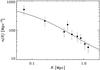 |
Fig. 8 Projected number density profile of zp-selected cluster members (points with 1σ error bars) and the best-fit model (projected-NFW + constant density background; solid curve). The reduced χ2 of the fit is 0.8. |
Since the uncertainties on rn are very large, we also considered an alternative estimate based on the spectroscopic sample of cluster members (see Sect. 5.1). The radial geometrical completeness, Cg(R), is the same for this sample as for the zp-selected sample. In addition, the spectroscopic sample suffers from radially dependent completeness because the fraction of galaxies with measured redshifts is higher near the cluster center. We evaluated this spectroscopic completeness, Cs(R), as the ratio of the number of galaxies with measured redshifts to the total number of galaxies (134 and 713 in total) in radial bins, down to F814 ≤ 23. We found Cs(R) = 0.22 outside the central bin, that is, at R ≥ 0.11 arcmin, and Cs(R) = 0.50 inside this bin. We then ran a maximum-likelihood fit of the spatial distribution of spectroscopic members weighting each galaxy by [Cg(Ri) × Cs(Ri)] -1. We found  Mpc, and a background density corresponding to 4% background contamination. The background contamination is much lower than for the zp-selected sample, as expected. The rn value is consistent within the (large) error bars with that were obtained using the zp-selected sample.
In the dynamical analysis with the DK and MAMPOSSt methods, we used both estimates of rn to understand to which degree our limited knowledge of rn affects our estimate of the cluster mass profile. The knowledge of rn is not required for the dynamical analysis with the caustic method.
5.3. Results
For the DK and MAMPOSSt methods we used the NFW model for M(r) (Navarro et al. 1997),  (10)where c200 ≡ r200/r-2 is the mass profile concentration. The model has two free parameters, the virial mass and concentration, or, equivalently, the virial and scale radii r200 and r-2. Note that the total mass density scale-length is different from the scale radius of the galaxy number density profile, that is, r-2 ≠ rn (Sect. 5.2), since we allowed the distribution of the total mass and that of the galaxies to be different in our analysis. For the caustic technique, we also fit an NFW model to the mass density profile determined from differentiation of the non-parametrically determined mass profile for comparison with the other two methods.
The MAMPOSSt method is the only one among the three with complete freedom in the choice of β(r). We used a simplified version of the model of Tiret et al. (2007), β(r) = β∞r/ (r + r-2), where β∞ is the asymptotic value of the anisotropy reached at large radii, and r-2 is the scale radius of the NFW mass density distribution. This model was shown by Mamon et al. (2010) to provide a good fit to cluster-mass halos extracted from cosmological numerical simulations. In this model, galaxy orbits are isotropic near the cluster center and become increasingly radially anisotropic outside.
In the caustic technique, we used Gaussian adaptive kernels for the density estimation in projected phase space, with an initial kernel size equal to the optimal kernel size of Silverman (1986). Before the density estimation, we scaled the velocity coordinates such that the scaled velocity dispersion is the same as the dispersion in the radial coordinates. In the equation that connects M(r) to the caustic amplitude (Eq. (13) in Diaferio 1999), we adopted either ℱβ = 0.5 as recommended by Diaferio (1999) and Geller et al. (2013), or ℱβ = 0.7 as recommended by Serra et al. (2011). To estimate the M(r) error we adopted the recipe of Diaferio (1999). Serra et al. (2011) have found that these error estimates correspond to 50% confidence levels; we therefore scaled them up by a factor of 1.4 to have ~1σ level error estimates. The chosen caustic is displayed in Fig. 6.
The domain of application of the DK and MAMPOSSt methods is the virial region. Since almost all our cluster members are in the virial region, we only excluded the very central region, 25 kpc, where the gravitational potential is probably dominated by the cD and therefore unlikely to follow a purely NFW profile.
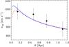 |
Fig. 9 Observed line-of-sight velocity dispersion profile (points with 1σ error bars) and those predicted by the best-fit NFW models, obtained with the DK (dashed red line), and MAMPOSSt (solid blue line) methods. Only solutions obtained using the rn value found with the zp sample of members are shown for clarity. |
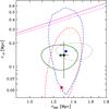 |
Fig. 10 Best-fit M(r) NFW parameters from the kinematics analyses within 1σ confidence level contours, obtained with the DK (red squares), MAMPOSSt (blue dot and circle), and caustic methods (green filled and open diamond). The filled (open) symbols are for the solutions obtained using the rn value from the photometric (spectroscopic) sample of members. The dashed red (dash-dotted blue) contour represents the 1σ confidence region on the best-fit parameters of the DK (MAMPOSSt) method, obtained using the rn value from the photometric sample of members. The solid (dotted) green contour represents the 1σ confidence region on the best-fit parameters for the caustic method obtained using ℱβ = 0.5 (resp. ℱβ = 0.7). The magenta solid (dash-dotted) inclined line is the theoretical predictions for relaxed clusters at the mean redshift of LCDCS 0504 from Bhattacharya et al. (2013) (De Boni et al. 2013). The black dot with error bars is the weighted average of the DK, MAMPOSSt, and caustic results. |
The results of the dynamical analysis are summarized in Table 5 and displayed in Fig. 10, where we show the confidence contour in the [r200,r-2] plane. We also list and display a weighted average of the DK, MAMPOSSt, and caustic results. We multiplied the formal error on this average by  to take into account that the five averaged results are not independent. The constraints on the β parameters obtained by the DK and MAMPOSSt methods are very loose, therefore we do not display them here.
The values of r200 obtained by the DK, MAMPOSSt, and caustic methods agree well. The caustic solution obtained with ℱβ = 0.5 is closer to those from the other two methods. This would argue in favor of using this value instead of ℱβ = 0.7 in the caustic technique, as done recently by Geller et al. (2013). However, Gifford et al. (2013) recently suggested using the intermediate value ℱβ=0.65. Moreover, for β = cst NFW models, at the half-mass radius of ≈2 r-2, ℱβ = 0.5 corresponds to β = −1.1, while ℱβ = 0.7 corresponds to β = 0.3. The very tangential anisotropy for ℱβ = 0.5 is different from what most analyses extract for galaxies in clusters (e.g. Biviano et al. 2013, and references therein), so the agreement of the ℱβ = 0.5 solution with those of the DK and MAMPOSSt methods may be merely fortuitous.
The DK and MAMPOSSt methods pose very weak constraints on r-2. Mamon et al. (2013) already noted that the determination of the dark matter scale radius is inefficient, which Sanchis et al. (2004) had previously noted for the concentration parameter. The constraints obtained by the caustic technique are tighter and almost independent of the value of ℱβ. The caustic technique is able to better constrain the r-2 parameter of the mass distribution than the DK and MAMPOSSt techniques possibly because, unlike these, it is the only free parameter in the model fit. In fact, β(r) is fixed when the value of ℱβ is assumed, and r200 is estimated nonparametrically directly from the Caustic mass profile.
The agreement between the MAMPOSSt and DK solutions is also evident in Fig. 9, where we show the projection of the best-fit DK and MAMPOSSt solutions on the observed line-of-sight velocity dispersion profile9.
In Fig. 10 we also show the theoretical predictions of Bhattacharya et al. (2013) and De Boni et al. (2013) for the concentration-mass relation of relaxed clusters at the redshift of LCDCS 0504, converted in the r200-r-2 plane. Both theoretical predictions derive too high a concentration for a cluster of the mass and at the redshift of LCDCS 0504. Since the prediction of De Boni et al. (2013) is based on hydrodynamic simulations while that of Bhattacharya et al. (2013) originates from DM-only simulations, the discrepancy between theoretical predictions and observation cannot be explained by baryonic processes affecting the cluster dynamical structure.
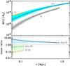 |
Fig. 11 Top panel: mass profiles and their 1 σ confidence regions obtained from the SL (red dashed line and yellow region), X-ray (black dashed line and gray region), and kinematics (blue solid line and cyan region) analyses. Bottom panel: ratios of the three mass profiles and their 1σ confidence regions. Solid blue line and gray-cyan region: ratio of the kinematics to X-ray mass profiles. Dashed-dotted blue line and green region: ratio of the kinematics to SL mass profiles. Dashed black line and orange region: ratio of the X-ray to SL mass profiles. In both panels the profiles are shown in the radial range where they are constrained by the data. |
6. Comparing the different mass profile determinations
The methods based on SL, X-ray, and kinematics to determine the cluster mass profile have different sensitivities on different scales. It would therefore be misleading to either extrapolate the SL and X-ray mass estimates to r200 to compare them with the result from kinematics, or to restrict the spectroscopic data-sample to a smaller region to directly infer r2500 or r500 from the kinematics analysis, with loss of statistics. Instead of comparing the mass profile parameters, a more appropriate comparison is that between the different mass profiles themselves in the regions where they overlap.
The three M(r) from the SL, X-ray, and kinematics analyses are shown in the top panel of Fig. 11, their ratios are shown in the bottom panel of the same figure10. The SL and kinematics M(r) agree within the errors. The significant difference in the r200 values of these two profiles is therefore due to the uncertain extrapolation of the SL M(r), which is considerably flatter than the kinematics M(r). On the other hand, within inner 100 kpc, the M(r) obtained by the X-ray analysis is significantly lower than either the SL or kinematics mass profiles. In this case, the discrepancy is real and cannot be attributed to extrapolation uncertainties.
We discuss the possible origin of the differences between the mass profiles in Sect. 8.
7. Gas mass fraction
We computed the intracluster gas mass profile with the integral of the gas density profile of Eq. (6) over a spherical volume. For the present cluster we have  (11)where
  is the standard hypergeometric function11.
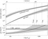 |
Fig. 12 Top panel: intracluster gas mass profile (lower curve) and the hydrodynamical derived total mass radial profiles. The gray-shaded regions represent 1σ confidence levels. Vertical lines indicate rimage, the limit where the cluster is detected with the combined XMM data (using both exposures), and r500 and r200, computed from the X-ray derived mass profile. Bottom panel: gas mass fraction radial profile. As a reference we also show the universal gas fraction, as obtained by the cosmic baryon fraction Ωb/ Ωm value from WMAP-9yr (Hinshaw et al. 2013) and Planck 1st release (Planck Collaboration XVI 2014, including their uncertainties), reduced by 17%. |
 |
Fig. 13 Top panel: ratio of gas mass to total mass from the X-ray analysis. The gray-shaded region within solid lines is the 1σ interval on the observed gas mass fraction of LCDCS 0504. The blue- and red-shaded regions (the blue one below the red one at large radii) are the average gas mass fractions for cool-core and non-cool-core clusters from Eckert et al. (2013). Bottom panel: ratio of gas mass to total mass, the latter derived from the kinematics analysis. The gray-shaded region within solid lines is the 1σ interval on the observed gas mass fraction of LCDCS 0504. The green-shaded region is the average gas mass fraction for nearby clusters from Biviano & Salucci (2006). |
Dividing Eqs. (11) by (7) yields the gas mass fraction, fgas. Figure 12 shows the mass profiles, gas and total, in the upper panel and the gas fraction radial profile in the bottom panel. The cluster gas mass fraction increases with r, as seen in most clusters (see, e.g., Biviano & Salucci 2006; Allen et al. 2008; Frederiksen et al. 2009). At r> 300 kpc, the gas mass fraction reaches a value that is consistent with the cosmic gas fraction, which is ≃83% of the cosmic baryon fraction (Fukugita et al. 1998; Hinshaw et al. 2013; Planck Collaboration XVI 2014).
A comparison with the results of Eckert et al. (2013) shows that the gas mass fraction profile of LCDCS 0504 is very similar to that of lower-z clusters, except near the cluster center, where it is significantly lower. This is shown in the top panel of Fig. 13 where we plot the results of Eckert et al. (2013) for the average gas mass fraction of cool-core and non-cool-core clusters together with our results, based in both cases on the total mass determined from X-ray analysis. If we instead use the total mass determined from kinematics, we can compare our result with that of Biviano & Salucci (2006). This comparison is shown in the bottom panel of Fig. 13. In this case the gas fraction of LCDCS 0504 appears to lie below that for a sample of nearby clusters at almost all radii.
Finally, we compared the LCDCS 0504 gas mass fraction computed using the total mass derived from our lensing analysis (see Sect. 3) with those of Zhang et al. (2010), also derived using total mass estimates from lensing, except that they used the weak-lensing, not the strong-lensing effect. The comparison is shown in Fig. 14, where we plot the gas mass fractions as a function of the cluster mass, both determined at r2500. This is the smallest radius at which Zhang et al. (2010) have given their determinations, and it is still outside the region where SL is detected in LCDCS 0504, r2500 = 0.49 Mpc for the SL M(r). From Fig. 14 we see that the gas mass fraction of LCDCS 0504 at this radius is not anomalous. This is consistent with the conclusions we obtained using the X-ray- and kinematics-determined total masses (Fig. 13), LCDCS 0504 shows an anomalous (low) gas mass fraction only at small radii.
We discuss in the next section the possible origin of this central gas fraction deficiency.
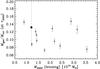 |
Fig. 14 Ratio of gas mass to total mass determined from lensing analyses for the clusters of Zhang et al. (2010) (diamonds) and for LCDCS 0504 (dot). Error bars are 1σ. |
8. Discussion and conclusions
We have analyzed the mass profile M(r) of a z ≈ 0.8 cluster with the SL technique, using the X-ray emission from the intracluster hot gas, and using galaxies as tracers of the gravitational potential. The different determinations of the cluster M(r) disagree, especially in the inner regions. The SL M(r) is slightly higher than but still consistent with the kinematic determination, but both are significantly higher than the X-ray M(r) determination.
This discrepancy is probably not caused by an unrelaxed dynamical status of the cluster. This might cause an overestimate of the cluster velocity dispersion and hence the cluster mass estimate from kinematics (see, e.g., Biviano et al. 2006) and an incomplete thermalization of the intracluster gas, leading to an underestimate of the cluster mass estimates from X-ray (e.g. Rasia et al. 2006), but it would not affect the lensing mass estimate. Moreover, an unrelaxed dynamical status is not supported by the analyses of substructures by Guennou et al. (2014). In that paper, we used the Serna & Gerbal (1996, SG hereafter) hierarchical method for the detection of substructures in the distribution of galaxies and searched for substructures in the X-ray data (described in Sect. 2.1), by analyzing the residuals of the subtraction of a symmetric elliptical β-model from the X-ray image (see Guennou et al. 2014, for details). Seven substructures were detected by the SG technique, all with masses lower than 10% of the total cluster mass. Of these, only one was also detected in X-rays, with an X-ray luminosity of ≈8% of the total cluster X-ray luminosity. This analysis indicates that any major perturbation of the LCDCS 0504 dynamical status must thus have occurred sufficiently long ago for the remnants of the merging groups to have disappeared.
Another interesting possibility is that we see the cluster with its major axis along the line-of-sight. This is suggested by the circularly symmetric SL configuration and by the small ellipticity of the cD galaxy, since the elongation of cD galaxies generally reflects those of their host clusters (e.g. Rhee & Katgert 1987; Kim et al. 2002) (see Fig. 1). It has been shown in numerical simulations (Kasun & Evrard 2005) and observationally (Wojtak 2013) that clusters are prolate not only in position space, but also in velocity space, and the major axes of the spatial and velocity distributions are aligned. The orientation of the cluster with the major axis along the line-of-sight then results in an overestimate of the cluster mass estimatd from SL and velocity dispersion. According to Wojtak (2013), the mean ratio of the velocity dispersions along the minor and major axes of a cluster is ≃0.78. This implies a ratio of the velocity dispersion along the major axis to the mean cluster velocity dispersion of 1.16, that is, a 32% mass overestimate at a given radius. This is still not sufficient to remove the systematic difference between the mass profile derived from kinematics and that derived by the X-ray analysis.
The alignment effect just discussed might also induce an overestimate of mass profile concentration value. This might explain the disagreement we found with the theoretical predictions of Bhattacharya et al. (2013) and De Boni et al. (2013, see Fig. 10).
Whatever the cause for the X-ray vs. kinematics and SL M(r) discrepancy, substantial systematic underestimates of cluster masses by the X-ray methodology might be interesting for cosmology because it might alleviate the tension between the σ8 values found by the Planck collaboration using the cosmic microwave background power-spectrum on one hand and cluster counts obtained by the Sunyaev-Zeldovich effect (using X-ray masses as mass calibrators Planck Collaboration XX 2014): if X-ray masses are underestimated at given SZ signal, this means the distribution of SZ counts above a given mass threshold is underestimated, meaning that Ωm (σ8) is underestimated (overestimated), which would bring the best-fit value more in line with the CMB value.
Another intriguing result of our analysis is the discovery that the gas mass fraction is anomalously low near the center of the LCDCS 0504 cluster. Given the relaxed, symmetric morphology of the X-ray emission (see Fig. 3), it is unlikely that this anomaly can be attributed to the effects of a major merger displacing the gas from the center, as in the case of the Bullet cluster (Barrena et al. 2002; Markevitch et al. 2002). Alternatively, the gas might have been ejected by AGN outbursts, while the effects of SNe explosions are expected to be insignificant (Conroy & Ostriker 2008; Dubois et al. 2013). Dubois et al. (2013) predicted a 30% loss in the core due to AGN outflows, which is not to far from our observed deficiency (with respect to the average of other clusters) of ≃60% (see Fig. 13), given the large observational uncertainties.
The main problem with the AGN hypothesis is that there is no evidence of a radio source in the NVSS catalog or in the X-rays because there is no detectable point source at the location of the cD, although there is a hint of a cool core. In addition, we have no evidence of broad lines in the optical spectrum of the cD. This lack of evidence does tell us, however, that the assumed AGN activity has subsided long enough ago that all strong electromagnetic signatures of AGN activity have now subsided.
In the near future, we plan to extend the dynamical and structural analysis presented here to clusters with sufficient spectroscopic information in the full DAFT/FADA cluster set. Expanding our data-sets will allow us to determine whether the anomalies identified in LCDCS 0504 are a characteristic of high-z clusters or not. Hopefully, with a larger sample we will be able to unveil the hidden systematics that cause discrepant determinations of cluster mass profiles by different methods, and to relate these systematics to the currently poorly understood physics of the intracluster baryons.
Online material
Coordinates, magnitudes, and redshifts of the LCDCS 0504 spectroscopic galaxy catalog.
Science Analysis System from the XMM-Newton team, http://xmm.esac.esa.int/sas/current/sas_news.shtml
We used βX for the parameter of the model to distinguish it from the kinematics β, see Eq. (9). (Cavaliere & Fusco-Femiano 1976), with a flat background added to it.
For each galaxy in the cluster, R is the projected cluster-centric distance from the cD galaxy, and vrf is the rest-frame velocity vrf ≡ (v − vcl) / (1 + vcl/c), where vcl is the mean velocity of the cluster. This is re-defined at each new iteration of the membership selection, until convergence. The cluster center is defined to be the position of the cD galaxy.
We recall that the DK best-fit solution is obtained by a simultaneous fit of both the observed velocity dispersion profile and the observed kurtosis profile, while the MAMPOSSt best-fit solution is obtained by a fit of the full line-of-sight velocity distribution. Figure 9 is just a way of presenting the best-fit models.
For βX = 1 / 2, consistent with our fit to the X-ray surface brightness profile, a useful approximation to the hypergeometric function of Eq. (11) is ![\hbox{${}_2F_1\left(\frac{3}{2},\frac{3}{4},\frac{5}{2}, - \frac{r^2}{r_c^2} \right) \simeq 6 \left [(x^3/3)^{-\gamma}+(2 x^3/3)^{-\gamma}\right]^{-1/\gamma}$}](/articles/aa/full_html/2014/06/aa22447-13/aa22447-13-eq171.png) , where γ = 21 / 8 ≃ 1.0905, which is accurate to better than 2.7% for all radii (see Mamon & Łokas 2005).
, where γ = 21 / 8 ≃ 1.0905, which is accurate to better than 2.7% for all radii (see Mamon & Łokas 2005).
Acknowledgments
We wish to express our sincere condolences and grief to the family of Alain Mazure, who unexpectedly passed away during the preparation of this paper. We wish to thank the anonymous referee for her/his suggestions. Based on XMM-Newton archive data and on data retrieved from the NASA/IPAC Extragalactic Database (NED) which is operated by the Jet Propulsion Laboratory, California Institute of Technology, under contract with the National Aeronautics and Space Administration. Also based on observations made with the FORS2 multi-object spectrograph mounted on the Antu VLT telescope at ESO-Paranal Observatory (programme 175.A-0706(B)). Also based on observations obtained at the Gemini Observatory, which is operated by the Association of Universities for Research in Astronomy, Inc., under a cooperative agreement with the NSF on behalf of the Gemini partnership: the National Science Foundation (United States), the Science and Technology Facilities Council (United Kingdom), the National Research Council (Canada), CONICYT (Chile), the Australian Research Council (Australia), Ministério da Ciência, Tecnologia e Inovação (Brazil) and Ministerio de Ciencia, Tecnología e Inovación Productiva (Argentina). Finally, this research has made use of the VizieR catalog access tool, CDS, Strasbourg, France. Also based on observations made with the NASA/ESA Hubble Space Telescope, obtained from the data archive at the Space Telescope Science Institute. STScI is operated by the Association of Universities for Research in Astronomy, Inc. under NASA contract NAS 5-26555. Also based on visiting astronomer observations, at Cerro Tololo Inter-American Observatory, National Optical Astronomy Observatory, which is operated by the Association of Universities for Research in Astronomy, under contract with the National Science Foundation. This work has been carried out thanks to the support of the Labex OCEVU (ANR-11-LABX-0060) and the A*MIDEX (ANR-11-IDEX-0001-02) funded by the “Investments for the Future” French government program managed by the French National Research Agency (ANR). M.L. acknowledges the Centre National de la Recherche Scientifique (CNRS) for its support. The Dark Cosmology Centre is funded by the Danish National Research Foundation. This work has been conducted using facilities offered by CeSAM (Centre de donnéeS Astrophysique de Marseille – http://www.lam.fr/cesam/). F.D. acknowledges long-term support from CNES and CAPES/COFECUB program 711/11. A.B. acknowledges the hospitality of the Inst. d’Astroph. de Paris and of the Obs. de la Côte d’Azur. This research has made use of the NASA/IPAC Extragalactic Database (NED), which is operated by the Jet Propulsion Laboratory, California Institute of Technology, under contract with the National Aeronautics and Space Administration. G.B.L.N. and ESC acknowledge the support of the Brazilian funding agencies FAPESP and CNPq. Based on observations obtained at the Gemini Observatory, which is operated by the Association of Universities for Research in Astronomy, Inc., under a cooperative agreement with the NSF on behalf of the Gemini partnership: the National Science Foundation (United States), the National Research Council (Canada), CONICYT (Chile), the Australian Research Council (Australia), Ministério da Ciência, Tecnologia e Inovação (Brazil) and Ministerio de Ciencia, Tecnología e Innovación Productiva (Argentina). I.M. acknowledges financial support from the Spanish grant AYA2010-15169 and from the Junta de Andalucia through TIC-114 and the Excellence Project P08-TIC-03531.
References
- Adami, C., Biviano, A., Durret, F., & Mazure, A. 2005, A&A, 443, 17 [NASA ADS] [CrossRef] [EDP Sciences] [Google Scholar]
- Allen, S. W., Rapetti, D. A., Schmidt, R. W., et al. 2008, MNRAS, 383, 879 [NASA ADS] [CrossRef] [Google Scholar]
- Anders, E., & Grevesse, N. 1989, Geochim. Cosmochim. Acta, 53, 197 [Google Scholar]
- Balucinska-Church, M., & McCammon, D. 1992, ApJ, 400, 699 [NASA ADS] [CrossRef] [Google Scholar]
- Bardeau, S., Kneib, J., Czoske, O., et al. 2005, A&A, 434, 433 [NASA ADS] [CrossRef] [EDP Sciences] [Google Scholar]
- Barrena, R., Biviano, A., Ramella, M., Falco, E. E., & Seitz, S. 2002, A&A, 386, 816 [NASA ADS] [CrossRef] [EDP Sciences] [Google Scholar]
- Bartelmann, M. 1996, A&A, 313, 697 [NASA ADS] [Google Scholar]
- Beers, T. C., Flynn, K., & Gebhardt, K. 1990, AJ, 100, 32 [NASA ADS] [CrossRef] [Google Scholar]
- Bhattacharya, S., Habib, S., Heitmann, K., & Vikhlinin, A. 2013, ApJ, 766, 32 [NASA ADS] [CrossRef] [Google Scholar]
- Binney, J., & Tremaine, S. 1987, Galactic dynamics (Princeton: Princeton University Press), 747 [Google Scholar]
- Biviano, A. 2006, in EAS Publ. Ser. 20, eds. G. A. Mamon, F. Combes, C. Deffayet, & B. Fort, 171 [Google Scholar]
- Biviano, A., & Girardi, M. 2003, ApJ, 585, 205 [NASA ADS] [CrossRef] [Google Scholar]
- Biviano, A., & Katgert, P. 2004, A&A, 424, 779 [NASA ADS] [CrossRef] [EDP Sciences] [Google Scholar]
- Biviano, A., & Salucci, P. 2006, A&A, 452, 75 [NASA ADS] [CrossRef] [EDP Sciences] [Google Scholar]
- Biviano, A., Durret, F., Gerbal, D., et al. 1996, A&A, 311, 95 [NASA ADS] [Google Scholar]
- Biviano, A., Murante, G., Borgani, S., et al. 2006, A&A, 456, 23 [NASA ADS] [CrossRef] [EDP Sciences] [Google Scholar]
- Biviano, A., Rosati, P., Balestra, I., et al. 2013, A&A, 558, A1 [NASA ADS] [CrossRef] [EDP Sciences] [Google Scholar]
- Böhringer, H., Pratt, G. W., Arnaud, M., et al. 2010, A&A, 514, A32 [NASA ADS] [CrossRef] [EDP Sciences] [Google Scholar]
- Borgani, S., & Guzzo, L. 2001, Nature, 409, 39 [NASA ADS] [CrossRef] [PubMed] [Google Scholar]
- Briel, U. G., Henry, J. P., Schwarz, R. A., et al. 1991, A&A, 246, L10 [NASA ADS] [Google Scholar]
- Cavaliere, A., & Fusco-Femiano, R. 1976, A&A, 49, 137 [NASA ADS] [Google Scholar]
- Coe, D., Benítez, N., Broadhurst, T., & Moustakas, L. A. 2010, ApJ, 723, 1678 [NASA ADS] [CrossRef] [Google Scholar]
- Conroy, C., & Ostriker, J. P. 2008, ApJ, 681, 151 [NASA ADS] [CrossRef] [Google Scholar]
- Cypriano, E. S., Sodré, Jr., L., Kneib, J.-P., & Campusano, L. E. 2004, ApJ, 613, 95 [NASA ADS] [CrossRef] [Google Scholar]
- De Boni, C., Ettori, S., Dolag, K., & Moscardini, L. 2013, MNRAS, 428, 2921 [NASA ADS] [CrossRef] [Google Scholar]
- DeCarlo, L. T. 1997, Psychol. Methods, 2, 292 [CrossRef] [Google Scholar]
- den Hartog, R., & Katgert, P. 1996, MNRAS, 279, 349 [NASA ADS] [CrossRef] [Google Scholar]
- Diaferio, A. 1999, MNRAS, 309, 610 [NASA ADS] [CrossRef] [Google Scholar]
- Diaferio, A., & Geller, M. J. 1997, ApJ, 481, 633 [NASA ADS] [CrossRef] [Google Scholar]
- Dressler, A., & Shectman, S. A. 1988, AJ, 95, 985 [NASA ADS] [CrossRef] [Google Scholar]
- Dubois, Y., Pichon, C., Devriendt, J., et al. 2013, MNRAS, 428, 2885 [NASA ADS] [CrossRef] [Google Scholar]
- Eckert, D., Ettori, S., Molendi, S., Vazza, F., & Paltani, S. 2013, A&A, 551, A23 [NASA ADS] [CrossRef] [EDP Sciences] [Google Scholar]
- Elíasdóttir, Á., Limousin, M., Richard, J., et al. 2007, unpublished [arXiv:0710.5636] [Google Scholar]
- Escalera, E., Biviano, A., Girardi, M., et al. 1994, ApJ, 423, 539 [NASA ADS] [CrossRef] [Google Scholar]
- Frederiksen, T. F., Hansen, S. H., Host, O., & Roncadelli, M. 2009, ApJ, 700, 1603 [NASA ADS] [CrossRef] [Google Scholar]
- Fukugita, M., Hogan, C. J., & Peebles, P. J. E. 1998, ApJ, 503, 518 [NASA ADS] [CrossRef] [Google Scholar]
- Geller, M. J., Diaferio, A., Rines, K. J., & Serra, A. L. 2013, ApJ, 764, 58 [NASA ADS] [CrossRef] [Google Scholar]
- Gifford, D., Miller, C., & Kern, N. 2013, ApJ, 773, 116 [NASA ADS] [CrossRef] [Google Scholar]
- Girardi, M., & Biviano, A. 2002, Optical Analysis of Cluster Mergers, ASSL, Merging Processes in Galaxy Clusters), 272, 39 [Google Scholar]
- Guennou, L., Adami, C., Ulmer, M. P., et al. 2010, A&A, 523, A21 [NASA ADS] [CrossRef] [EDP Sciences] [Google Scholar]
- Guennou, L., Adami, C., Durret, F., et al. 2014, A&A, 561, A112 [NASA ADS] [CrossRef] [EDP Sciences] [Google Scholar]
- Halliday, C., Milvang-Jensen, B., Poirier, S., et al. 2004, A&A, 427, 397 [NASA ADS] [CrossRef] [EDP Sciences] [Google Scholar]
- Hinshaw, G., Larson, D., Komatsu, E., et al. 2013, ApJS, 208, 19 [NASA ADS] [CrossRef] [Google Scholar]
- Jee, M. J., White, R. L., Benítez, N., et al. 2005, ApJ, 618, 46 [NASA ADS] [CrossRef] [Google Scholar]
- Johnson, O., Best, P., Zaritsky, D., et al. 2006, MNRAS, 371, 1777 [NASA ADS] [CrossRef] [Google Scholar]
- Jullo, E., Kneib, J.-P., Limousin, M., et al. 2007, New J. Phys., 9, 447 [Google Scholar]
- Kaastra, J. S., & Mewe, R. 1993, A&AS, 97, 443 [NASA ADS] [Google Scholar]
- Kalberla, P. M. W., Burton, W. B., Hartmann, D., et al. 2005, A&A, 440, 775 [NASA ADS] [CrossRef] [EDP Sciences] [Google Scholar]
- Kasun, S. F., & Evrard, A. E. 2005, ApJ, 629, 781 [NASA ADS] [CrossRef] [Google Scholar]
- Katgert, P., Biviano, A., & Mazure, A. 2004, ApJ, 600, 657 [NASA ADS] [CrossRef] [Google Scholar]
- Kent, S. M., & Gunn, J. E. 1982, AJ, 87, 945 [NASA ADS] [CrossRef] [Google Scholar]
- Kim, R. S. J., Annis, J., Strauss, M. A., & Lupton, R. H. 2002, in Tracing Cosmic Evolution with Galaxy Clusters, eds. S. Borgani, M. Mezzetti, & R. Valdarnini, ASP Conf. Ser., 268, 395 [Google Scholar]
- Leonard, A., King, L. J., & Goldberg, D. M. 2011, MNRAS, 413, 789 [NASA ADS] [CrossRef] [Google Scholar]
- Liedahl, D. A., Osterheld, A. L., & Goldstein, W. H. 1995, ApJ, 438, L115 [NASA ADS] [CrossRef] [Google Scholar]
- Limousin, M., Kneib, J.-P., & Natarajan, P. 2005, MNRAS, 356, 309 [NASA ADS] [CrossRef] [Google Scholar]
- Limousin, M., Kneib, J. P., Bardeau, S., et al. 2007a, A&A, 461, 881 [NASA ADS] [CrossRef] [EDP Sciences] [Google Scholar]
- Limousin, M., Richard, J., Jullo, E., et al. 2007b, ApJ, 668, 643 [NASA ADS] [CrossRef] [Google Scholar]
- Łokas, E. L., & Mamon, G. A. 2001, MNRAS, 321, 155 [NASA ADS] [CrossRef] [Google Scholar]
- Łokas, E. L., & Mamon, G. A. 2003, MNRAS, 343, 401 [NASA ADS] [CrossRef] [Google Scholar]
- Łokas, E. L., Wojtak, R., Gottlöber, S., Mamon, G. A., & Prada, F. 2006, MNRAS, 367, 1463 [NASA ADS] [CrossRef] [Google Scholar]
- Mamon, G. A., & Łokas, E. L. 2005, MNRAS, 363, 705 [NASA ADS] [CrossRef] [Google Scholar]
- Mamon, G. A., Biviano, A., & Murante, G. 2010, A&A, 520, A30 [NASA ADS] [CrossRef] [EDP Sciences] [Google Scholar]
- Mamon, G. A., Biviano, A., & Boué, G. 2013, MNRAS, 429, 3079 [NASA ADS] [CrossRef] [Google Scholar]
- Markevitch, M., Gonzalez, A. H., David, L., et al. 2002, ApJ, 567, L27 [NASA ADS] [CrossRef] [Google Scholar]
- Markevitch, M., Gonzalez, A. H., Clowe, D., et al. 2004, ApJ, 606, 819 [NASA ADS] [CrossRef] [Google Scholar]
- Mohr, J. J., Fabricant, D. G., & Geller, M. J. 1993, ApJ, 413, 492 [NASA ADS] [CrossRef] [Google Scholar]
- Navarro, J. F., Frenk, C. S., & White, S. D. M. 1997, ApJ, 490, 493 [NASA ADS] [CrossRef] [Google Scholar]
- Nelson, A. E., Gonzalez, A. H., Zaritsky, D., & Dalcanton, J. J. 2001, ApJ, 563, 629 [NASA ADS] [CrossRef] [Google Scholar]
- Neumann, D. M., Arnaud, M., Gastaud, R., et al. 2001, A&A, 365, L74 [NASA ADS] [CrossRef] [EDP Sciences] [Google Scholar]
- O’Hara, T. B., Mohr, J. J., & Guerrero, M. A. 2004, ApJ, 604, 604 [NASA ADS] [CrossRef] [Google Scholar]
- Planck Collaboration XVI. 2014, A&A, in press, DOI: 10.1051/0004-6361/201321591 [Google Scholar]
- Planck Collaboration XX. 2014, A&A, in press, DOI: 10.1051/0004-6361/201321521 [Google Scholar]
- Pratt, G. W., Böhringer, H., & Finoguenov, A. 2005, A&A, 433, 777 [NASA ADS] [CrossRef] [EDP Sciences] [Google Scholar]
- Ramella, M., Biviano, A., Pisani, A., et al. 2007, A&A, 470, 39 [NASA ADS] [CrossRef] [EDP Sciences] [Google Scholar]
- Rasia, E., Ettori, S., Moscardini, L., et al. 2006, MNRAS, 369, 2013 [NASA ADS] [CrossRef] [Google Scholar]
- Rhee, G. F. R. N., & Katgert, P. 1987, A&A, 183, 217 [NASA ADS] [Google Scholar]
- Sanchis, T., Łokas, E. L., & Mamon, G. A. 2004, MNRAS, 347, 1198 [NASA ADS] [CrossRef] [Google Scholar]
- Serna, A., & Gerbal, D. 1996, A&A, 309, 65 [NASA ADS] [Google Scholar]
- Serra, A. L., Diaferio, A., Murante, G., & Borgani, S. 2011, MNRAS, 412, 800 [NASA ADS] [Google Scholar]
- Silverman, B. W. 1986, Density estimation for statistics and data analysis (Landon: Chapman and Hall) [Google Scholar]
- Tiret, O., Combes, F., Angus, G. W., Famaey, B., & Zhao, H. S. 2007, A&A, 476, L1 [NASA ADS] [CrossRef] [EDP Sciences] [Google Scholar]
- van der Marel, R. P., Magorrian, J., Carlberg, R. G., Yee, H. K. C., & Ellingson, E. 2000, AJ, 119, 2038 [NASA ADS] [CrossRef] [Google Scholar]
- Wojtak, R. 2013, A&A, 559, A89 [NASA ADS] [CrossRef] [EDP Sciences] [Google Scholar]
- Wojtak, R., & Łokas, E. L. 2010, MNRAS, 408, 2442 [NASA ADS] [CrossRef] [Google Scholar]
- Wojtak, R., Łokas, E. L., Mamon, G. A., et al. 2007, A&A, 466, 437 [NASA ADS] [CrossRef] [EDP Sciences] [Google Scholar]
- Wojtak, R., Łokas, E. L., Mamon, G. A., & Gottlöber, S. 2009, MNRAS, 399, 812 [NASA ADS] [CrossRef] [Google Scholar]
- Zhang, Y.-Y., Okabe, N., Finoguenov, A., et al. 2010, ApJ, 711, 1033 [NASA ADS] [CrossRef] [Google Scholar]
All Tables
Coordinates, magnitudes, and redshifts of the LCDCS 0504 spectroscopic galaxy catalog.
All Figures
|
Fig. 1 HST image of the core of LCDCS 0504. The size of the field is 38 × 34 arcsec2, corresponding to 285 × 255 kpc2 at z = 0.794. Multiple imaged systems used in this work are labeled. From the best-fit strong-lensing model, we draw in red the tangential critical curve at z = 3 and the corresponding caustic lines in orange. |
| In the text | |
|
Fig. 2 Summed spectrum of arcs 1.1, 1.2, and 1.3. The best redshift is 3.005. |
| In the text | |
|
Fig. 3 XMM-Newton image using all available data. The cluster is shown inside the yellow central circle of radius equal to 30′′. The other visible X-ray sources are point-source AGNs. |
| In the text | |
|
Fig. 4 2D surface brightness fit. Left: LCDCS 0504 image in the [0.5–7.0 keV] band with point sources and artifacts (CCD gap) masked out. Middle: best-fit β-model (see text for details) shown with the same color coding as the original image. Right: residuals, data minus best-fit model. No apparent structure is seen in the residual image. |
| In the text | |
|
Fig. 5 Best-fit absorbed MEKAL model. Top: all detectors from both XMM-Newton observation are fitted simultaneously, as described in the text. Bottom: plot of the residual contribution to the χ2 per energy bin of the best-fit spectrum. |
| In the text | |
|
Fig. 6 Projected phase space distribution of galaxies with redshifts in the cluster region. Selected cluster members are shown as filled dots. The chosen caustic in the caustic method is shown in green. |
| In the text | |
|
Fig. 7 Adaptive-kernel-smoothed distribution of photometric redshifts for galaxies in the cluster region. The vertical (blue) line shows the average cluster redshift. The solid (red) curve shows the selected zp range for the sample used to determine n(r). |
| In the text | |
|
Fig. 8 Projected number density profile of zp-selected cluster members (points with 1σ error bars) and the best-fit model (projected-NFW + constant density background; solid curve). The reduced χ2 of the fit is 0.8. |
| In the text | |
|
Fig. 9 Observed line-of-sight velocity dispersion profile (points with 1σ error bars) and those predicted by the best-fit NFW models, obtained with the DK (dashed red line), and MAMPOSSt (solid blue line) methods. Only solutions obtained using the rn value found with the zp sample of members are shown for clarity. |
| In the text | |
|
Fig. 10 Best-fit M(r) NFW parameters from the kinematics analyses within 1σ confidence level contours, obtained with the DK (red squares), MAMPOSSt (blue dot and circle), and caustic methods (green filled and open diamond). The filled (open) symbols are for the solutions obtained using the rn value from the photometric (spectroscopic) sample of members. The dashed red (dash-dotted blue) contour represents the 1σ confidence region on the best-fit parameters of the DK (MAMPOSSt) method, obtained using the rn value from the photometric sample of members. The solid (dotted) green contour represents the 1σ confidence region on the best-fit parameters for the caustic method obtained using ℱβ = 0.5 (resp. ℱβ = 0.7). The magenta solid (dash-dotted) inclined line is the theoretical predictions for relaxed clusters at the mean redshift of LCDCS 0504 from Bhattacharya et al. (2013) (De Boni et al. 2013). The black dot with error bars is the weighted average of the DK, MAMPOSSt, and caustic results. |
| In the text | |
|
Fig. 11 Top panel: mass profiles and their 1 σ confidence regions obtained from the SL (red dashed line and yellow region), X-ray (black dashed line and gray region), and kinematics (blue solid line and cyan region) analyses. Bottom panel: ratios of the three mass profiles and their 1σ confidence regions. Solid blue line and gray-cyan region: ratio of the kinematics to X-ray mass profiles. Dashed-dotted blue line and green region: ratio of the kinematics to SL mass profiles. Dashed black line and orange region: ratio of the X-ray to SL mass profiles. In both panels the profiles are shown in the radial range where they are constrained by the data. |
| In the text | |
|
Fig. 12 Top panel: intracluster gas mass profile (lower curve) and the hydrodynamical derived total mass radial profiles. The gray-shaded regions represent 1σ confidence levels. Vertical lines indicate rimage, the limit where the cluster is detected with the combined XMM data (using both exposures), and r500 and r200, computed from the X-ray derived mass profile. Bottom panel: gas mass fraction radial profile. As a reference we also show the universal gas fraction, as obtained by the cosmic baryon fraction Ωb/ Ωm value from WMAP-9yr (Hinshaw et al. 2013) and Planck 1st release (Planck Collaboration XVI 2014, including their uncertainties), reduced by 17%. |
| In the text | |
|
Fig. 13 Top panel: ratio of gas mass to total mass from the X-ray analysis. The gray-shaded region within solid lines is the 1σ interval on the observed gas mass fraction of LCDCS 0504. The blue- and red-shaded regions (the blue one below the red one at large radii) are the average gas mass fractions for cool-core and non-cool-core clusters from Eckert et al. (2013). Bottom panel: ratio of gas mass to total mass, the latter derived from the kinematics analysis. The gray-shaded region within solid lines is the 1σ interval on the observed gas mass fraction of LCDCS 0504. The green-shaded region is the average gas mass fraction for nearby clusters from Biviano & Salucci (2006). |
| In the text | |
|
Fig. 14 Ratio of gas mass to total mass determined from lensing analyses for the clusters of Zhang et al. (2010) (diamonds) and for LCDCS 0504 (dot). Error bars are 1σ. |
| In the text | |
Current usage metrics show cumulative count of Article Views (full-text article views including HTML views, PDF and ePub downloads, according to the available data) and Abstracts Views on Vision4Press platform.
Data correspond to usage on the plateform after 2015. The current usage metrics is available 48-96 hours after online publication and is updated daily on week days.
Initial download of the metrics may take a while.