| Issue |
A&A
Volume 563, March 2014
|
|
|---|---|---|
| Article Number | A41 | |
| Number of page(s) | 14 | |
| Section | Planets and planetary systems | |
| DOI | https://doi.org/10.1051/0004-6361/201322374 | |
| Published online | 03 March 2014 | |
The GTC exoplanet transit spectroscopy survey
I. OSIRIS transmission spectroscopy of the short period planet WASP-43b⋆,⋆⋆
1
Instituto de Astrofísica de Canarias (IAC),
38205
La Laguna, Tenerife
Spain
e-mail:
murgas_ext@iac.es
2
Departamento de Astrofísica, Universidad de La Laguna
(ULL), 38206, La
Laguna, Tenerife,
Spain
3
Centro de Astrobiología (CSIC-INTA), 28850 Torrejón de
Ardoz, Madrid,
Spain
4
Institut für Astrophysik, Georg-August-Universität,
Friederich-Hund-Platz 1,
37077
Göttingen,
Germany
Received: 26 July 2013
Accepted: 9 January 2014
Aims. In this work, we use long-slit spectroscopy observations of a transit event of the close-in orbiting planet WASP-43b (Mp = 2.034 MJup, Rp = 1.036 RJup) in an effort to detect its atmosphere.
Methods. We used the Gran Telescopio Canarias (GTC) instrument OSIRIS to obtain long-slit spectra in the optical range 520–1040 nm of the planetary host star WASP-43 and of a reference star during a full primary transit event and four partial transit observations. We integrated the stellar flux of both stars in different wavelength regions producing several light curves. We fitted transit models to these curves to measure the star-to-planet radius ratio, Rp/Rs, across wavelength among other physical parameters.
Results. We measure a mean planet-to-star radius ratio in the white light curve of 0.15988-0.00145+0.00133. Using broadband filters, we detect the color signature of WASP-43. We present a tentative detection in the planet-to-star radius ratio around the Na i doublet (λ 588.9, 589.5 nm) when compared to the nearby continuum at the 2.9σ level. We find no significant excess of the measured planet-to-star radius ratio around the K i doublet (λ 766.5 nm, 769.9 nm) when compared to the nearby continuum. Combining our observations with previously published epochs, we refine the estimation of the orbital period. Using a linear ephemeris, we obtained a period of P = 0.81347385 ± 1.5 × 10⁻⁷ days. Using a quadratic ephemeris, we obtained an orbital period of 0.81347688 ± 8.6 × 10⁻⁷ days, and a change in this parameter of Ṗ = −0.15 ± 0.06 s/year. As previous results, this hints to the orbital decay of this planet although a timing analysis over several years needs to be made to confirm this.
Key words: planets and satellites: atmospheres / planets and satellites: gaseous planets / techniques: spectroscopic
Photometry is only available at the CDS via anonymous ftp to cdsarc.u-strasbg.fr (130.79.128.5) or via http://cdsarc.u-strasbg.fr/viz-bin/qcat?J/A+A/563/A41
Appendix is available in electronic form at http://www.aanda.org
© ESO, 2014
1. Introduction
Among the increasing family of extrasolar planets discovered so far, only a handful of them possess orbital periods of less than a day. Some examples of close-in exoplanets include possible disintegrating planets (KIC 12557548b, Rappaport et al. 2012), super-Earths (Corot-7b, Léger et al. 2009; 55 Cnc e, McArthur et al. 2004, Dawson & Fabrycky 2010, Winn et al. 2011), and hot Jupiters (WASP-18b, Hellier et al. 2009; WASP-19b, Hebb et al. 2009; WASP-43b, Hellier et al. 2011; and WTS-2b, Birkby et al. 2014). The study of these close-in orbiting planets can shed some light in the dynamic interactions that produce planetary migrations, tidal interactions between the star and the planet, and in the case of transiting hot Jupiters, they offer a good opportunity to study the atmospheric composition of extrasolar planets under extreme stellar irradiation.
The planet WASP-43b was discovered by the Wide Angle Search of Planets team in 2011 (Hellier et al. 2011). It orbits a K7V star with an estimated mass of 0.717 ± 0.025 M⊙ and a stellar radius of 0.667 ± 0.011 R⊙ (Gillon et al. 2012). Gillon et al. (2012) presented a study of several transits observed with TRAPPIST (TRAnsiting Planets and PlanetesImals Small Telescope), Very Large Telescope (VLT) near-IR photometry, and CORALIE radial velocities. They improved the parameters of the system finding an eccentricity consistent with a circular orbit (e = 0), a semi-major axis over stellar radius of  , and an estimated planetary mass and radius of 2.034 ± 0.052 MJup and 1.036 ± 0.019 RJup, respectively. By using secondary eclipse observations, the thermal emission of the planet at 1.16 μm and 2.09 μm was detected. Blecic et al. (2014) measured the secondary eclipse of WASP-43b in the 3.6 μm and 4.5 μm bands using Spitzer, deducing a planetary brightness temperature of 1684 ± 24 K and 1485 ± 24 K, respectively. Wang et al. (2013) also detected the secondary eclipse in the H and Ks bands from the ground using the Wide-field Infrared Array Camera (WIRCam) mounted at the Canada-France-Hawaii Telescope (CFHT); their data are consistent with a blackbody with a temperature of 1850 K, higher than the expected equilibrium temperature of the planet.
Blecic et al. (2014) also improved the Gillon et al. (2012) estimation of the orbital period by a factor of three, finding a period of P = 0.81347459 ± 2.1 × 10⁻⁷ days. With such a short period of less than a day, WASP-43b is expected to move towards smaller orbits over time, and to eventually fall into the star on a timescale between 8–800 Myr depending on the efficiency of orbital energy dissipation from the star (Hellier et al. 2011). Because of its close orbit around its host star and its considerable size when compared to the stellar radius, WASP-43b offers a good opportunity to study this planet’s atmosphere using current ground-based instrumentation.
One of the most successful techniques used to infer the atmospheric composition of extrasolar planets is transmission spectroscopy. When a planet transits its host star, part of the starlight will be absorbed by the atoms and molecules present in the planetary atmosphere. Since atoms and molecules absorb radiation at specific energies, they will produce variations in the flux transmitted through the atmosphere. A direct consequence of these flux variations will be the change in the measured depth of the transit at specific wavelengths. Given their large sizes compared to their host stars, hot Jupiters are excellent targets for transmission spectroscopy studies, mainly because they produce a deep transit and, since they are gaseous planets, they possess large atmospheres with considerable scale heights. Some successful examples of transmission spectroscopy have been the detection of sodium from space and the ground in the systems HD 209458b (Charbonneau et al. 2002; Snellen et al. 2008) and HD 189733b (Redfield et al. 2008); the study of short-period hot Jupiters in the near-IR (e.g. Bean et al. 2013), and the study of super-Earths (e.g., Bean et al. 2010, 2011).
Here, we probe the atmosphere of WASP-43b by means of transmission spectroscopy of one full and four partial planetary transit events. In Sect. 2 we describe the observation setup; in Sect. 3 we describe the data reduction process to produce the final light curves, and the light curve fitting methodology; in Sect. 4 we present the results of the data analysis; and in Sect. 5 we present the conclusions of our work.
2. Observations
The Gran Telescopio Canarias (GTC) is a 10.4 m telescope located at Observatorio Roque de los Muchachos in La Palma. The GTC instrument OSIRIS (Optical System for Imaging and low Resolution Integrated Spectroscopy, Cepa et al. 2000) consists of two charge couple devices (CCD) detectors with a field of view (FOV) of 7.8 × 7.8 arcmin and plate scale of 0.127 arcsec/pix. The GTC/OSIRIS instrument has been used successfully for planetary science in the past, using broadband photometry (e.g., Tingley et al. 2011), tunable filter observations (e.g., Sing et al. 2011, Colón et al. 2012b, Murgas et al. 2012), and long-slit transmission spectroscopy (e.g., Sing et al. 2012).
For our observations, we chose the 2 × 2 binning mode, a readout speed of 200 kHz with a gain of 0.95 e-/ADU and a readout noise of 4.5 e-. We used OSIRIS in its long-slit spectroscopic mode, selecting the grism R1000R which covers the spectral range of 520–1040 nm, and a custom-built slit width of 12 arcsec. With such a wide slit, the spectral resolution is dominated by the seeing during the observations, which varied between 0.8 and 1.8 arcsec. This translates in an effective spectral resolution of R = 374–841 at 751 nm. The use of a wider slit has the advantage of reducing the possible systematic effects that can be introduced by light losses due to changes in seeing, airmass, and/or losses caused by differential telescope guiding between the two stars.
Data for WASP-43b were taken in visiting mode on January 8, 2013. As reference we chose 2MASS J10200126-0948099 (J = 10.16 mag, KS = 9.62 mag), a star with a similar R-band magnitude and located at a distance of 5.74 arcmin from the target. Owing to the FOV of OSIRIS, the target and reference star had to be located in separate CCDs. The position angle of the reference star with respect to the target (measured east of north) was PA = 2.39°. Observations began at 02:28 UT (one hour before ingress) and ended at 05:30 UT (one hour after egress). The exposure time was set to 15 s and the readout time of the instrument was close to 21 s, meaning we collected approximately one spectrum every 36 s. Spectra of the target star and the reference star were not collected at parallactic angle. However, given the large size of the slit width, the red wavelengths covered by our instrumental setup, and the airmasses of the observations (secz = 1.45–1.35 with a minimum at 1.28 near mid-transit), no significant flux losses due to the Earth’s atmospheric refraction are expected. Nevertheless, because the seeing varied during the observations, we applied a correction as explained in Sect. 3.
In addition to the data taken in January 2013 (set 5 from now on), we have four more transit observations taken with GTC/OSIRIS on December 22, 2011 (set 1); February 8, 2012 (set 2); February 21, 2012 (set 3); and April 18, 2012 (set 4). These observations were made using a different electronic configuration: the readout speed was set to 500 kHz with a gain of 1.46 e-/ADU and a readout noise of 8.0 e-. We decided to use this readout configuration to obtain a higher time cadence. Unfortunately, none of these observations were of the expected quality. In particular, during the observations of set 1, 3, and 4 part of the flux was lost or the observations were interrupted due to technical problems with the telescope, while set 2 was observed under bad weather conditions. These old data sets were not adequate to perform a transmission spectroscopy study, but they can be used to search for the color signature variation from transit to transit, and to fit a transit model to the white light curves in order to obtain the central time of the eclipse. For posterior observations we changed to the 200 kHz readout speed to minimize the electronic noise associated with a faster read while not sacrificing the cadence of the data acquisition too much. This read mode has become the standard for GTC long-slit spectroscopy observations.
3. Methods
3.1. Data reduction
The raw data reduction was made using standard procedures. We combined bias and flat images using the Image Reduction and Analysis Facility (IRAF1) to produce the basic calibration frames, and used these calibration images to correct the science frames before the extraction of the spectra.
The extraction and wavelength calibration was made using a PyRAF2 script written for GTC/OSIRIS long-slit data. This script automatized some of the steps to produced the spectra, such as extraction of each spectrum, extraction of the corresponding calibration arc, wavelength calibration (using the HgAr, Xe, Ne lamps provided for the observations), and Doppler shift to take into account the possible shifts in wavelength due to the different radial velocities of the target and the chosen reference star. Given the low spectral resolution of our data, small to moderate errors in wavelength calibration do not introduce large uncertainties in the results presented here.
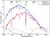 |
Fig. 1 Extracted R1000R grism spectrum of WASP-43 (red) and its reference star (blue). The spectra are not corrected for instrumental response or flux calibrated. Some stellar (black) and atmospheric O2 telluric features are shown (green). The V, R, I, and z sloan filters are also plotted in an arbitrary scale to show the wavelength coverage of the spectrum. |
Several apertures for the optimal extraction of the spectra were tested during the reduction process and the one that delivered the best results in terms of low scatter measured using the root mean square (rms) of the points outside of transit (after normalization) for the white light curve was selected. The results presented here for data set 5 were obtained using an aperture width of 50 pixels, which corresponds to 12.7 arcsec on the detector. This is 7 to 14 times the raw seeing during the observations.
The UT time of data acquisition was obtained using the recorded headers of the spectra indicating the opening and closing time of the shutter in order to compute the time of mid exposure. Then, we used the code written by Eastman et al. (2010)3 to compute the barycentric Julian date (BJD) in barycentric dynamical time using the mid exposure time for each of the spectra to produce the light curves analyzed here.
Figure 1 presents an example of an extracted spectrum of WASP-43 and the reference star used in the time series. The two spectra are not corrected for instrumental response nor are they flux calibrated.
3.2. Filter definition
The light curves were obtained using the numerical method known as Simpson’s rule (Press et al. 2002) to integrate the fluxes of each spectrum of the time series and take the ratio between the integrated flux of the target and the reference star. To explore the presence of atmospheric features in WASP-43b, we created several filters of different widths in wavelength domain.
In the case of the white light curve, the flux was integrated between 530 nm and 900 nm. Figure 2 presents the white light curve for data set 5 and Fig. 3 shows the white light curves for the previous GTC/OSIRIS sets.
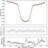 |
Fig. 2 Top panel: GTC/OSIRIS WASP-43b transit white light curve. The red line represents the best fit determined using our MCMC analysis. Middle panel: residuals of the fit. Bottom panel: full width at half maximum (FWHM) of WASP-43 in the spatial direction versus time, showing the seeing variations during the observations. |
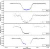 |
Fig. 3 GTC/OSIRIS white light curves for WASP-43b for data sets 1 to 4. Blue crosses in sets 1 and 4 show data that were taken when the telescope presented technical problems. |
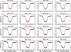 |
Fig. 4 Light curves obtained using the 25 nm filters for GTC set 5. The red line shows the best fit found by the MCMC analysis. |
In order to get the transmission spectrum of WASP-43b, the observed spectra of WASP-43 and its reference star were integrated using 25 nm filters a wavelength range between 530 nm and 900 nm, resulting in 16 light curves to be fitted (see Fig. 4). To test the robustness of the results found with the 25 nm filters, we produced 34 light curves using 10 nm filters with a wavelength range of 549.5–882 nm. The 10 nm bin centered at 589.6 nm has a width big enough to cover the Na i 588.9 and 589.5 nm doublet. In addition to these 25 nm and 10 nm bins, we produced nine curves using 18 nm filters to cover the region near the K i 766.5 and 769.9 nm doublet (wavelength range 702.0–855.5 nm).
To study the color signature of WASP-43 we defined two broad filters, one at the blue end of the observed spectra and one at the red end (530–680 nm and 800–950 nm, respectively). The filter coverage for the color signature is illustrated in the top panel of Fig. 7.
3.3. Light curve fitting
In order to get the transit parameters from the light curves (such as the planet-to-star radius ratio Rp/Rs) of set 5, we followed a Markov chain Monte Carlo (MCMC) Bayesian approach to get the distribution of probabilities of the fitted parameters and adopted the median of the distribution as the best fitted value (see Berta et al. 2012 and appendix for details).
To fit the white light curve, we assumed a circular orbit (eccentricity e = 0), fixed the orbital period to P = 0.81347459 days (taken from Blecic et al. 2014) and set as free parameters the planet-to-star radius ratio Rp/Rs, the quadratic limb darkening coefficients u1 and u2, the central time of the transit Tc, the orbital semi-major axis over stellar radius a/Rs, and the orbital inclination i.
To take into account the systematic effects induced by atmospheric extinction (and other effects observed in the curves obtained when we integrated the spectrum in wavelength), a third-degree polynomial with a time dependency was fitted to the data. In addition, a first-degree polynomial with a dependency on the measured full width at half maximum (FWHM) across the spatial direction of each spectrum was fitted to take into account the flux variability produced by changes in seeing during the observations. Although this last effect is not so evident in the white light curve of set 5, it affected more strongly the light curves obtained using narrower filters. To be self consistent with the analysis of curves presented here, we fitted this seeing dependency to all the obtained light curves.
Thus, the observed flux ratio was modeled by  (1)where
  is a synthetic transit model dependent on the transit parameters VT,
  polynomial dependent on time (t), and
  a polynomial with a seeing (s) dependency (in units of FWHM).
As a test, we computed the Bayesian Information Criterion (BIC; see Eq. (5)) for the white light curve to compare the use of a second- and a third-degree time-dependent polynomial (plus a linear function with a seeing dependency) to fit the systematic effects present in set 5. The BIC value for the third-degree polynomial was 74 while for the second-degree polynomial it was 70, meaning that the simpler model is slightly preferred, although the fit for the curve was better using the third-degree polynomial. As a final test, we fitted the 16 light curves produced using 25 nm filters using both parametrizations; the results were the same within the 1σ level of confidence. Since the choice of a second- or third-degree time-dependent polynomial did not affect our results, we decided to use the third-degree parametrization to fit all the light curves because it delivered a better fit to the systematic effects based on the rms of the residuals.
The procedure to fit the light curve was split into two step. Since out of the transit we have  , we first performed an MCMC simulation to obtain the coefficients of the third-degree time-dependent polynomial and the first-degree seeing dependent polynomial (and their corresponding 1σ error) using only the out-of-transit points. We used these values as a prior information to penalize the likelihood ℒ in order to fit the transit light curve model and the polynomials simultaneously in the next step of the fitting process.
In order to fit the white light curve and the functions to take into account the systematic effects, the second step started with a χ2 minimization. To generate the transit models we used a fast Python implementation of the Giménez (2006) code written by Hannu Parviainen4, which has been used in previous planetary studies (e.g., Murgas et al. 2012; Parviainen et al. 2013). As a starting point of the minimization we used the transit parameters of Gillon et al. (2012), the polynomial coefficients found in the first step, and for the limb darkening, the bolometric quadratic limb darkening coefficients of Claret (2000). For the limb darkening coefficients we used as a starting point of the fit the values of Claret (2000) computed for a star with a turbulent velocity of VT = 0 km s-1, log g = 4.5 cm/s2, Teff = 4500 K, and log (M/H) = 0.0 dex; these values are close to the values reported for WASP-43 by Hellier et al. (2011) and Gillon et al. (2012). We adopted the standard deviation of normalized residuals (SDNR), which is the rms of the points outside the transit after normalizing this baseline to unity, as the photometric error in the light curve. In the case of the white light curve of set 5, the SDNR of the points outside the transit was 543.7 ppm.
Once we had the best set of parameters that minimized the χ2 function, we used them as a starting point of the MCMC chains that computed the posterior probability distribution of the fitted parameters. There were a total of twelve fitted parameters: six transit parameters, five polynomial coefficients, and one scalar multiplying the rms of the out-of-transit points to find the best error of the light curve (see appendix). All twelve parameters were fitted simultaneously.
To run the MCMC chains, we chose the Python code emcee (Foreman-Mackey et al. 2013). This code provides a relatively fast, robust way of producing several independent chains. The different chains are created by slightly changing the solution that minimize the χ2 function. These different solutions will act as seeds to start the chains; that way we obtain a more robust result if all the chains (with different starting points) converge to the same probability distribution.
We used 300 independent chains (each one with twelve free parameters) and computed 3200 iterations per chain. In terms of iterations, this is the same as computing one chain 9.6 × 10⁵ times. To obtain the probability distribution from the chains, we left out the first 500 iterations as a burn-in period (the stage where the chains are still converging) and computed the cross-correlation length for each of the parameters. This way we only used independent samples from the chains to obtain the distributions. Then, each of the 300 chains with the selected independent samples, were merged into one to get the probability distribution of the fitted parameters. The final values and errors for the parameters were obtained by computing the percentiles of the distributions to get the median and standard deviation for each parameter.
For the filters of several widths used to produce different light curves, the fitting process was similar to the one used to fit the white light curve, with the difference that we fixed two of the geometric transit parameters (a/Rs, i) using the results of the white light curve fit. For the broadband filters, we used the Claret (2000) broadband quadratic limb darkening coefficients for the corresponding filters as a starting point for the minimization. For the smaller filters (10, 18, and 25 nm), we also used the Claret (2000) broadband quadratic limb darkening coefficients as a starting point to fit the light curve, changing the theoretical coefficient values with the corresponding wavelength of the center at the filters.
Figure 5 presents three curves with the transit removed from set 5 made with 25 nm filters and centered at 542.5, 767.5, and 867.5 nm, respectively. The red line shows the best fit for the time and seeing dependent polynomial found by the MCMC analysis. The seeing variations had a greater effect on the curves produced using the blue and red wavelength regions (see appendix). The strong improvement in the model fits when introducing the seeing dependence is indicative that even with a 12 arcsec slit width slit losses can still occur.
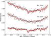 |
Fig. 5 Example of three light curves produced using the 25 nm filters for GTC set 5 with the transit removed and overplotted with a red line the best fit to take into account the systematic effects. The light curves at the red and blue end of the spectrum were more affected by flux losses caused by seeing variations. |
3.4. Red noise estimation
Time correlated noise, or red noise, can cause an underestimation of the errors in the fitted parameters of a light curve. To test for red noise in our data, we followed the procedure of Winn et al. (2008) which compares the predicted rms of the residuals of the fitted light curve versus the measured rms of the residuals of the curve binned in time. If the curve does not present red noise, the measured rms of the residuals when binning the light curve in time should follow the equation  (2)where σ1 is the rms of the residuals of the unbinned light curve, σN is the rms of the residuals of the curve binned in time, N is the number of points in the binned light curve, and M is the number of bins. We measured the rms of the residuals using M = 89 different bin sizes between 5 and 80 min with a step of 0.85 min and compared the measured rms versus the predicted σN. For each of the light curves we computed β = σmeasured/σN and adopted the median β value for the bins on a scale time of under 20 min as a multiplying factor to the errors found by the MCMC. In the cases where β < 1, we set β ≡ 1 meaning that the error in these light curves was set by the MCMC procedure. For the white light curve we derived a βWL = 1.5.
MCMC results of the white light transit curve of WASP-43b.
A test performed to the residuals of the fitted light curves showed that we were able to adjust the main sources of noise present in the data (see appendix). Hence, the use of this β factor to increase our uncertainties should be enough to compensate the possible underestimation of errors caused by red noise.
4. Results
4.1. White light curves and timing analysis
The white light curve and the best fitted model from the MCMC procedure are presented in the top panel of Fig. 2 and the obtained transit parameters are given in Table 1. To account for the red noise, the uncertainties presented in Table 1 correspond to the 1σ errors from the MCMC distributions multiplied by the factor β discussed in Sect. 3 (βWL = 1.5). The SDNR of the fit presented in the middle panel of Fig. 2 is 372.2 ppm. The integrated flux of the target was ≈1.7 × 10⁸ photons, with this number the photon noise was 79 ppm. Comparing the photon noise to the SDNR of the whitle light curve, we can conclude that the noise level in our curve is a factor of ~4.7 higher than the theoretical limit. Using the parameters found for the white light curve of set 5, we derived a transit duration of 74.7 ± 2.0 min.
Since this planet is expected to present some degree of orbital decay caused by tidal interactions between the star and the planet (Hellier et al. 2011), it is important to determine and monitor the orbital period with high accuracy and over several years to detect possible variations in this parameter. With that goal in mind, we use the five white light curves presented in this work to obtain the central time of transit. For the fitting we use the Transit Analysis Package (TAP, Gazak et al. 2012) which implements an MCMC method to fit Mandel & Agol (2002) transit models and also includes a wavelet method (Carter & Winn 2009) to estimate the level of red noise in the photometric curves.
We fitted a circular orbit to all five GTC transits, and fixed i, a/Rs, and the quadratic limb darkening coefficients (u1 and u2) to the values obtained from the fit of the white light curve using set 5. The transit parameter a/Rs is not expected to change significantly during the time interval of the observations. For each epoch we allow the central time of the transit to vary and the results, together with 1σ errors, are presented in Table 2. The uncertainties for the central time of set 5 found by TAP are compatible at the 1σ level to the value found by our MCMC fitting process multiplied by the computed β factor.
We compute the observed minus calculated (O–C) diagram (Fig. 6, top panel) of the central times of the transits of WASP-43b using the ephemeris equation and the 23 transit midtimes presented by Gillon et al. (2012) together with the Tc we obtained from the five GTC light curves. A clear deviation from the predicted times can be seen for the GTC epochs. This can be explained by the cumulative error in the ephemeris equation, specially in the value of the orbital period. To correct this, we fit a linear and a quadratic regression to the time residuals. Both linear and quadratic fits are weighted by the uncertainties in the central times of the transits.
Transit analysis package (TAP) fitted central time of transit for all the GTC/OSIRIS data sets reported here.
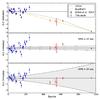 |
Fig. 6 Top panel: O–C diagram and linear and quadratic fits for GTC, Gillon et al. (2012) transits of WASP-43b. Middle panel: residuals of the linear fit to the data and 1σ uncertainties of fit (gray area). Bottom panel: residuals of the quadratic fit to the data and 1σ uncertainties of fit (gray area). |
After correcting for the linear trend, the updated linear ephemeris equation is  (3)where T0 = 2 455 528.8686144 ± 1.1 × 10⁻⁴ days and the resulting orbital period is P = 0.81347385 ± 1.5 × 10⁻⁷ days. The corrected O–C diagram is presented in the middle panel of Fig. 6. The rms of the timing residuals using the updated ephemeris equation is 37 s and
  of the linear fit is 5.1.
For the quadratic fit we use the same expression as Blecic et al. (2014),  (4)where T0 is a reference time, P the orbital period of the planet, N the number of transits since T0, and δP = ṖP with Ṗ a term describing the variation of the period.
The timing residual rms is 34 s if we use the quadratic regression fit (bottom panel, Fig. 6) with a  . The orbital period is P = 0.81347688 ± 8.6 × 10⁻⁷ days, the reference time is T0 = 2 455 528.8683108 ± 1.2 × 10⁻⁴ days, and Ṗ = −0.15 ± 0.06 s/year. Blecic et al. (2014) also found an indication of orbital decay with a Ṗ of − 0.65 ± 0.12 s/year, a factor 4.3 times bigger than the one found in our analysis.
To compare the results of the linear and quadratic fit, we also computed the Bayesian information criterion (BIC),  (5)where k is the number of free parameters of the fit and NP is the number of data points. The criterion favors the quadratic fit (BIC = 110.4) over the linear fit (BIC = 139.3). The preference of a quadratic fit to the timing data was also found by Blecic et al. (2014).
Considering the work of Blecic et al. (2014), this is the second study that suggests that there might be orbital decay in this particular planetary system. The period and orbital decay reported in Blecic et al. is a result based on the Tc from Gillon et al. (2012), their secondary transits from Spitzer, and amateur observations. We attribute the difference with our results to the different treatment of uncertainties in the reported central times to the method used to estimate the red noise and our longer baseline of timing observations. While Gillon et al. and Blecic et al. used time averaging methods, we have used the wavelet method which in principle delivers more conservative estimations of uncertainties (see Carter & Winn 2009, Sect. 4).
We tested this difference by simultaneously fitting three complete transits of WASP-43b reported by Gillon et al. (2012) using TAP. We found that the uncertainties we obtain are 1.5–2.0 times larger than the values originally reported. Similar results have been obtained when comparing the wavelet with time averaging methods (Hoyer et al. 2012, 2013).
The confirmation of orbital decay could help to constrain the stellar dissipation factor  (e.g. Rasio et al. 1996; Matsumura et al. 2010) and establish the survival time of the planet. Confirmation for WASP-43b needs to be done by a dedicated study of timing variations with a longer time baseline and a more uniform data analysis, hence the detection of orbital decay in this system remains an open question.
4.2. Color signature
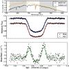 |
Fig. 7 Color signature of WASP-43. Top panel: spectrum of WASP-43 and reference star showing the regions where the blue and red filters were defined (gray area). Middle panel: blue and red light curves after correcting for systematic effects and best model fit. Bottom panel: color (blue-red) showing the color signature of WASP-43, the green line represents the difference of the fitted models for the blue and red filters. |
Simultaneous multicolor photometry of planetary transits has some very interesting applications such as the identification of false positives in searches for exoplanets and limb darkening studies of the host star (see Tingley 2004; Tingley et al. 2006; Colón et al. 2012a, and references therein).
As a planet transits the stellar disk it occults part of the stellar light and, due to the limb darkening effect, it will block more red light during the ingress and egress than during the middle of the transit. With simultaneous photometry in a blue and a red band it is possible to measure this effect by using the color blue-red measured during the transit.
As can be seen from in the bottom panel of Fig. 7, the effect of the color measurement (blue-red) of the transit creates horn-like structures in the ingress and egress of the transit. This effect is small, in this specific case with a peak near 1800 ppm. We also produced the blue and red light curves using the same broadband filters for the data sets 1 to 4; however, since these observations were not complete we did not fit a transit model. As shown in Fig. 8, we detect the same horn-like signature in several of the old GTC data sets. The overplotted model was taken from data set 5 and is consistent with the previous GTC observations.
The fitted limb darkening coefficients for the blue and red curves are u1Blue = 0.6057 ± 0.057, u2Blue = 0.1493 ± 0.071, u1Red = 0.3128 ± 0.056, and u2Red = 0.2415 ± 0.066. The coefficients of the blue curve are close to the Claret (2000) values for the R Johnson filter u1R = 0.6029 and u2R = 0.1418, while the coefficients for the red curve are slightly different from the values of Claret (2004) for the z sloan filter: u1z = 0.3834 and u2z = 0.227.
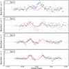 |
Fig. 8 Color signature of WASP-43: the same filters as Fig. 7, top panel, but using the old GTC data sets and overplotting the best fit for set 5 with a red line. Blue crosses in sets 1 and 4 show data that were taken when the telescope presented technical problems. |
4.3. Transmission spectroscopy
Figure 9 presents the results of the analysis using the 25 nm filters for the wavelength range of 530–900 nm. Table 3 presents the results of the measured Rp/Rs for each light curve, the corresponding 1σ uncertainties found by the MCMC, and the β factors to take into account the red noise for each curve.
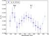 |
Fig. 9 Transmission spectrum of WASP-43b; the horizontal bars represent the wavelength width of the filters, the vertical error bar show the 1σ uncertainties found by the MCMC procedure after multiplying by the β factors to take into account the red noise. The last two points shown in light blue are probably affected by fringing. |
Rp/Rs, 1σ uncertainties from the MCMC analysis and β factors for the light curves produced using the 25 nm filters.
The first four bins present a maximum peak in the filter centered at 567.5 nm. Between 600 nm and 870 nm, the transmission spectrum presents a trend of an increase in the measured ratio Rp/Rs towards the red part of the spectrum (between 600 nm and 720 nm) and then the depth of the transit decreases until 880 nm. These trends observed with the 25 nm filters were also found in a test made with wider filters of 75 nm in width. We speculate that the increase in Rp/Rs between 620 nm and 720 nm and the posterior decrease redward of 720 nm may be consistent with a planet temperature in the range 1500–2000 K and the presence of molecular absorption due to VO and TiO, as shown by the isothermal model computations of Fortney et al. (2010), which assumed chemical equilibrium. This temperature range agrees with the values derived by Blecic et al. (2014) and Wang et al. (2013). According to the model spectra of Fortney et al. (2010), the presence of oxides make it harder to isolate the K i doublet with data of low spectral resolution; this is consistent with our finding. Detection of TiO and VO at optical wavelengths has also been claimed for HD 209458b (Désert et al. 2008), which has a warm dayside brightness temperature of 1320 ± 80 K (Crossfield et al. 2012).
The last two bins in the redder part of the spectrum centered at 892.5 nm and 917.5 nm present a higher Rp/Rs when compared to the adjacent filters; these bins could be more affected than the rest of the spectrum by fringing, although fringing patterns are not visible in our data. According to GTC staff5, fringing affects only at a 5% level for wavelengths λ > 930 nm and at less than 1% for wavelengths λ < 900 nm, but given the high precisions that transmission spectroscopy requires, it could be an important source of noise for red wavelengths when using the GTC R1000R grism.
To test the results obtained with 25 nm filters and to search for possible atmospheric features that the use of broad filters may have overlooked, we proceeded to create light curves using narrower filters in the regions near the Na i doublet, the K i doublet and the region between these two features where some telluric signals are located.
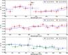 |
Fig. 10 Transmission spectrum of WASP-43b. The horizontal bars represent the width of the filters used to bin the spectrum and the vertical error bars represent the errors found by the MCMC procedure and the β factors to take into account the red noise. The gray line shows the extracted spectrum of WASP-43 in an arbitrary scale. Top panel: zoom to the Na i doublet region showing the results of the 25 nm (blue points) and 10 nm (red points) width filters; middle panel: same for the region between the Na and K lines; bottom panel: K i doublet region showing the 25 nm and 18 nm filter results. |
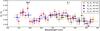 |
Fig. 11 Transmission spectrum of WASP-43b showing all the wavelength bins used in this study. The horizontal bars represent the wavelength width of the filters, the vertical error bars show the 1σ uncertainties found by the MCMC procedure after multiplying by the β factors to take into account the red noise. |
Figure 10, top panel, presents the comparison between the results using the light curves obtained with the 25 nm and 10 nm width filters for the region near the Na i doublet (see Table 4). We can see that the 10 nm width filter that possess the same center as the Na i doublet hints to an excess in the measured Rp/Rs when compared to the adjacent redder filters: however, the filters in the blue region next to the same line present a similar level of planetary radius to the one found in the Na feature. Using only the filter centered at 599.5 nm next to the Nai doublet, the difference between these two filters is Δ(Rp/Rs)Na−599.5 = (2.75 ± 0.84) × 10-3; if we use the filter centered at 579.5 nm we find a less significant excess of Δ(Rp/Rs)Na−579.5 = (1.53 ± 0.90) × 10-3. If we compute the weighted average (Rp/Rs) using the bins centered at 579.5 nm and 599.5 nm, we have (Rp/Rs)Avg = 0.16022 ± 4.51 × 10⁻⁴. Using this average value, Δ(Rp/Rs)Na−Avg = (2.18 ± 0.74) × 10-3, a 2.9σ significance excess. Assuming a stellar radius of Rs = 0.667 R⊙ (Gillon et al. 2012), this excess in Na could be traced back to an atmospheric height of Δ(Rp)Na−Avg = 1012 ± 344 Km.
Rp/Rs, 1σ uncertainties from the MCMC analysis and β factors for the light curves produced using the 10 nm filters near the Na i 588.9 nm and 589.5 nm doublet.
Rp/Rs, 1σ uncertainties from the MCMC analysis and β factors for the light curves produced using the 18 nm filters near the K i 766.5 nm and 769.9 nm doublet.
All these tests points to an excess in the measured planet-to-star radius ratio that could be produced by the atmosphere of WASP-43b, but our 2.9σ precision is not enough to claim an unambiguous detection. This tentative detection could be improved with new observations using, for example, the GTC/OSIRIS R1000B grism that covers a bluer part of the spectrum. Sodium has been detected in other exoplanets with slightly colder temperatures than WASP-43b like HD 209458b (Charbonneau et al. 2002), XO-2b (Sing et al. 2012) with a temperature of 1500 K (Machalek et al. 2009), and HD 189733b (Redfield et al. 2008) with an atmospheric temperature of 1340 ± 150 K (Lecavelier Des Etangs et al. 2008). The central panel of Fig. 10 shows an intermediate region between the Na i and K i doublet where we produced light curves using 10 nm filters. The planet-to-star radius ratio of the small filters are in agreement with the results found using 25 nm filters and present hints of an excess in Rp/Rs at the filters centered at 658 nm (near Hα) and 708 nm, but due to the errors in Rp/Rs we cannot claim a detection of the planet atmosphere in this region.
The bottom panel of Fig. 10 presents the wavelength region near K i doublet. The telluric absorption feature caused by O2 (see Fig. 1) is blended with the 766.5 and 769.9 nm potassium doublet at the resolution of our spectrum. One needs to be very careful not to confuse telluric variability from a possible planetary signature (see appendix). Thus, for this wavelength region, we chose a filter that was wider than the usual 10 nm filter used in the regions with shorter wavelengths in order to cover the entire oxygen and potassium lines. Taking the weighted average of the planet-to-star radius ratio of the two 18 nm of width filters adjacent to the K i doublet (747.0 nm and 783.0 nm) and using those bins as a pseudo-continuum, we found a difference between the line and the continuum of Δ(Rp/Rs)K−Avg = (0.755 ± 0.61) × 10-3, meaning that we do not detect a statistical significant excess in the measured Rp/Rs in the filter centered at the potassium doublet.
As a summary, Fig. 11 presents all the wavelength bins used to create the different light curves of WASP-43b. With our MCMC analysis and red noise estimation, the measured planet-to-star radius ratio agrees well for light curves created using filters of different widths in wavelength.
5. Conclusions and final remarks
In this work, we presented the results of GTC/OSIRIS long-slit spectroscopic observations of the extrasolar planet WASP-43b. Four partial transits taken on December 22, 2011; February 8, 2012; February 21, 2012; and April 18, 2012; and one full transit event observed on January 8, 2013 are analyzed. The observed wavelength range was 510–1040 nm and, in the case of the January 8, 2013 set, with a resolution of 374–841 at 751 nm.
Integrating the full range of wavelengths available in the observed spectrum of the target and its reference star, we produced a white light photometric curve. We fitted a transit model to data set 5 (full transit observations) and, using an MCMC analysis, we obtained transit parameters with their corresponding uncertainties that take into account the level of white and red noise in the photometric curve.
For each of the five GTC/OSIRIS WASP-43b data sets we fit the central time of the observed individual transits. Combining these results with previous observations made by Gillon et al. (2012), we see a decrease in time in the O–C versus epoch diagram. We attributed this trend to a cumulative error in the period determination ephemeris and proceeded to fit a linear and quadratic function to determine a new period. Using a linear fit, we find a new orbital period of P = 0.81347385±1.5 × 10⁻⁷ days. As reported by Blecic et al. (2014), the O–C data are better fitted using a quadratic function, with this parametrization we find an orbital period of P = 0.81347688±8.6 × 10⁻⁷ days and a change in the period of Ṗ = −0.15 ± 0.06 s/year. The Ṗ that we reported here is smaller than the one found by Blecic et al. (2014). Based on this discrepancy, a dedicated study of the transit timing of this system made over several years needs to be carried out in order to confirm the orbital decay of this particular planet.
Using blue and red light curves, we detected the classical horn-like structures representative of the color signature of WASP-43. We confirmed the color signature detection using the old GTC data sets. This shows the potential of performing multicolor studies using long-slit spectroscopy and transiting planets.
We also present here the transmission spectrum of WASP-43b using filters of 25, 18, and 10 nm in width. With the wider filters we observed a possible excess in Rp/Rs near the position of the Na i doublet, a trend of increasing planet-to-star radius ratio from blue to red wavelengths between 600 nm and 720 nm, and a decreasing Rp/Rs between 720 nm and 880 nm. The increase in Rp/Rs values between 620 nm and 720 nm and the decrease in Rp/Rs redward of 720 nm may be consistent with the temperature of WASP-43b and the presence of VO and TiO predicted by atmospheric models.
For the region near the Na i 588.9 nm and 589.5 nm doublet, we found an excess in Rp/Rs using filters of 10 nm in width. Taking the average of the Rp/Rs of the two adjacent filters as a continuum, we obtained a difference of Δ(Rp/Rs)Na−Avg = (2.18 ± 0.74) × 10-3, meaning that the excess is detected with 2.9σ of confidence. The regions in the blue part of the Na i doublet were more affected by flux losses due to seeing variations. In the region between 640 nm and 760 nm, we observed an increase in the measured planet-to-star radius ratio until the spectrum reaches the potassium doublet.
We probed the wavelength region near the K i doublet (766.5 nm, 769.9 nm) using filters of 18 nm in width. We do not detect a significant excess in the planet-to-star radius ratio at the position of the potassium doublet. After the K i doublet and until 855 nm, the bins follow a trend of a decreasing planet-to-star radius ratio.
According to the models of Fortney et al. (2010) sodium and potassium features are strong at planetary temperatures between 1000 and 1500 K, close to the brightness temperature found by Blecic et al. (2014) of T = 1684 ± 24 K and T = 1485 ± 24 K for the 3.6 μm and 4.5 μm Spitzer bands. Our data points to an excess in the measured planet-to-star radius in the Na i doublet and no detection of an excess in the K i doublet, which would make WASP-43b a planet with atmospheric characteristics similar to HD 209458b.
Online material
Appendix A: Extraction of the spectrum, data modeling, and red noise
Appendix A.1: Data reduction
During the data analysis of this work we found that the Rp/Rs measured in the filters centered at the potassium doublet were sensitive to the removal of bad pixels and/or cosmic rays. The IRAF routine used to extract the spectrum, APALL, presents the option of removing and replacing deviant pixels. The user can choose the threshold level at which to replace the pixels that present a lower sensitivity (bad pixels) or high values caused by cosmic rays. Since the O2 telluric feature is fairly deep, a lower threshold limit wrongfully identified the pixel that was near the minimum flux of the absorption line as a deviant pixel and replaced that pixel value. This occurred more or less randomly for both target and reference stars in the time series due to the changes in the depth of the telluric line caused by atmospheric variability. This effect produced extra noise in the light curve computed using a wavelength width of 25 and 18 nm around the K doublet.
The extra noise produced by the cleaning algorithm created a deeper and noisier transit in that filter and, with our MCMC, a spurious detection of potassium in WASP-43b. This problem was fixed by reducing the data several times, fine tuning the threshold level of rejection in order to detect and remove bad pixels and cosmic rays, but not replacing the values of the deepest points in the O2 absorption line. This delivered a higher quality light curve centered near the oxygen telluric line that presented a similar noise level to that seen in the curves of the adjacent wavelength regions.
It is also important to correctly parametrize the model to correct any flux variation that is correlated with some of the observational parameters like the seeing. In our first attempt to fit the data we did not consider seeing as a source of noise in the measured flux ratio between the target and reference star; that caused the MCMC to compute very large error bars in the measured Rp/Rs in the filters computed in the blue part of the spectrum and a flat transmission spectrum between 750 nm and 870 nm.
Figure A.1 shows a comparison of the results obtained using two different threshold levels to remove bad pixels and cosmic rays: a 6.5σ shown in red and the final 10σ rejection limit in blue. Both results were obtained without correcting for seeing variations and present a flat transmission spectrum in the red region next to the K doublet, unlike the results presented here in Figs. 9 and 10.
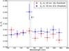 |
Fig. A.1 Comparison of results of the measured Rp/Rs around the potassium doublet using different threshold levels to remove bad pixels and cosmic rays, and no seeing correction in the light curve fitting process. A lower threshold level could produce a spurious detection of an excess in the planet-to-star radius ratio near a deep telluric line as shown by blue squares. The blue and red data points do not present the trend in decreasing Rp/Rs between 750 nm and 870 nm as unlike the results shown in Figs. 9 and 10. |
 |
Fig. A.2 Correlation plot showing the posterior distribution of the parameters fitted to the white light curve of WASP-43b. |
Appendix A.2: Data analysis
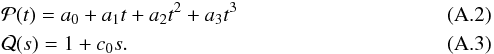
As we explained in Sect. 3.3, we fitted a transit model adding two polynomials to take into account the time and seeing dependent systematic effects present in the data,  (A.1)where is a synthetic transit model dependent on the transit parameters VT. For the white light curve VT = (Rp/Rs,u1,u2,Tc,a/Rs,i) with Rp/Rs the planet-to-star radius ratio, (u1,u2) the quadratic limb darkening coefficients, Tc the central time of the transit, a/Rs the semi-major axis over stellar radius, and i the orbital inclination;
  is a time-dependent polynomial, and
  a seeing dependent polynomial:
For the MCMC fitting procedure we followed a similar approach as Berta et al. (2012) and used as likelihood ℒ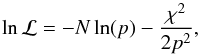 (A.4)where N is the number of points in the curve and p a coefficient to normalize the χ2. The function χ2 compares the data points with the model
 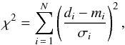 (A.5)where di is the data point, mi the model point, and σi the error in the measurement which in our case was assumed to be the SDNR of the points outside the transit.
The probability priors used for each parameter are presented in Table A.1. The use of a normal prior for the polynomial parameters to take into account the systematic effects was adopted using the information of the MCMC analysis performed using the points outside the transit.
Type of probability priors used in the analysis.
Figure A.2 presents a correlation plot for the posterior distribution of all the parameters used to fit the white light curve. The parameters that are more correlated with the planet-to-star radius ratio are the limb darkening coefficient u2, the semi-major axis over stellar radius a/Rs, and the orbital inclination i.
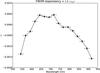 |
Fig. A.3 Seeing coefficient c0 as function of wavelength. The flux losses produced by seeing variations were stronger at both the blue and red ends of the detector. |
Figure A.3 shows the variation of the coefficient c0 used to fit the seeing variations according to Eq. (A.3). The coefficient
varies across wavelength, with a greater dependency on FWHM at both ends of the wavelength range of the detector.
Appendix A.3: Red noise analysis
To compare our error estimation with TAP (Gazak et al. 2012), we performed an analysis of the residuals of the fitted light curves using our MCMC method. The TAP method is based on the paper of Carter & Winn (2009) and computes the red noise contribution in the light curves. Their method is applied when the square of the Fourier transform of the residuals ( ) follow a power law
  (A.6)with A a constant, f the Fourier frequency, and γ the exponent of the power law. If γ = 0 we are in the presence of white noise; if γ = 1.0, pink noise; and if γ = 2.0, red noise.
We computed for the white light curve (see Fig. A.4) and the curves produced using the filters of 75 nm and 25 nm in width. In all the cases the residuals followed a power law with γ ≲ 0.3, indicating that with our fitting procedure the residuals are dominated by white noise. We can also conclude that this γ ≲ 0.3 regime is far from the assumed noise level of TAP (with γ = 1.0), meaning that in this particular case TAP could be overestimating the uncertainties. Since our fitting procedure is close to the white noise regime, we think that our estimation is more accurate than using TAP for this specific data set.
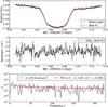 |
Fig. A.4 Red noise analysis. Top panel: white light curve of WASP-43b and best fit. Middle panel: residuals of the white light curve (curve after subtracting the best fit). Bottom panel: square of the Fourier transform of the residuals. A fit of the form A/fγ yields an exponent value of γ = 0.302; according to Carter & Winn (2009) this means that the major noise source in this curve is white noise. |
Acknowledgments
Based on observations made with the Gran Telescopio Canarias (GTC), installed in the Spanish Observatorio del Roque de los Muchachos of the Instituto de Astrofísica de Canarias, in the island of La Palma. S.H. acknowledges financial support from the Spanish Ministry of Economy and Competitiveness (MINECO) under the 2011 Severo Ochoa Program MINECO SEV-2011-0187. All the figures presented here were made using Matplotlib (Hunter 2007).
References
- Bean, J. L., Miller-Ricci Kempton, E., & Homeier, D. 2010, Nature, 468, 669 [NASA ADS] [CrossRef] [PubMed] [Google Scholar]
- Bean, J. L., Désert, J.-M., Kabath, P., et al. 2011, ApJ, 743, 92 [NASA ADS] [CrossRef] [Google Scholar]
- Bean, J. L., Désert, J.-M., Seifahrt, A., et al. 2013, ApJ, 771, 108 [NASA ADS] [CrossRef] [Google Scholar]
- Berta, Z. K., Charbonneau, D., Désert, J.-M., et al. 2012, ApJ, 747, 35 [NASA ADS] [CrossRef] [Google Scholar]
- Birkby, J. L., Capetta, M., Cruz, P., et al. 2014, MNRAS, submitted [Google Scholar]
- Blecic, J., Harrington, J., Madhusudhan, N., et al. 2014, ApJ, 781, 116 [NASA ADS] [CrossRef] [Google Scholar]
- Carter, J. A., & Winn, J. N. 2009, ApJ, 704, 51 [NASA ADS] [CrossRef] [Google Scholar]
- Cepa, J., Aguiar, M., Escalera, V. G., et al. 2000, in SPIE Conf. Ser. 4008, eds. M. Iye, & A. F. Moorwood, 623 [Google Scholar]
- Charbonneau, D., Brown, T. M., Noyes, R. W., & Gilliland, R. L. 2002, ApJ, 568, 377 [NASA ADS] [CrossRef] [Google Scholar]
- Claret, A. 2000, A&A, 363, 1081 [NASA ADS] [Google Scholar]
- Claret, A. 2004, A&A, 428, 1001 [NASA ADS] [CrossRef] [EDP Sciences] [Google Scholar]
- Colón, K. D., Ford, E. B., & Morehead, R. C. 2012a, MNRAS, 426, 342 [NASA ADS] [CrossRef] [Google Scholar]
- Colón, K. D., Ford, E. B., Redfield, S., et al. 2012b, MNRAS, 419, 2233 [NASA ADS] [CrossRef] [Google Scholar]
- Crossfield, I. J. M., Knutson, H., Fortney, J., et al. 2012, ApJ, 752, 81 [NASA ADS] [CrossRef] [Google Scholar]
- Dawson, R. I., & Fabrycky, D. C. 2010, ApJ, 722, 937 [NASA ADS] [CrossRef] [Google Scholar]
- Désert, J.-M., Vidal-Madjar, A., Lecavelier Des Etangs, A., et al. 2008, A&A, 492, 585 [NASA ADS] [CrossRef] [EDP Sciences] [Google Scholar]
- Eastman, J., Siverd, R., & Gaudi, B. S. 2010, PASP, 122, 935 [NASA ADS] [CrossRef] [Google Scholar]
- Foreman-Mackey, D., Hogg, D. W., Lang, D., & Goodman, J. 2013, PASP, 125, 306 [CrossRef] [Google Scholar]
- Fortney, J. J., Shabram, M., Showman, A. P., et al. 2010, ApJ, 709, 1396 [NASA ADS] [CrossRef] [Google Scholar]
- Gazak, J. Z., Johnson, J. A., Tonry, J., et al. 2012, Adv. Astron., 2012 [Google Scholar]
- Gillon, M., Triaud, A. H. M. J., Fortney, J. J., et al. 2012, A&A, 542, A4 [NASA ADS] [CrossRef] [EDP Sciences] [Google Scholar]
- Giménez, A. 2006, A&A, 450, 1231 [NASA ADS] [CrossRef] [EDP Sciences] [Google Scholar]
- Hebb, L., Collier-Cameron, A., Loeillet, B., et al. 2009, ApJ, 693, 1920 [NASA ADS] [CrossRef] [Google Scholar]
- Hellier, C., Anderson, D. R., Collier Cameron, A., et al. 2009, Nature, 460, 1098 [NASA ADS] [CrossRef] [Google Scholar]
- Hellier, C., Anderson, D. R., Collier Cameron, A., et al. 2011, A&A, 535, L7 [NASA ADS] [CrossRef] [EDP Sciences] [Google Scholar]
- Hoyer, S., Rojo, P., & López-Morales, M. 2012, ApJ, 748, 22 [NASA ADS] [CrossRef] [Google Scholar]
- Hoyer, S., Lopez-Morales, M., Rojo, P., et al. 2013, MNRAS, 434, 46 [NASA ADS] [CrossRef] [Google Scholar]
- Hunter, J. D. 2007, Comput. Sci. Eng., 9, 90 [Google Scholar]
- Lecavelier Des Etangs, A., Pont, F., Vidal-Madjar, A., & Sing, D. 2008, A&A, 481, L83 [NASA ADS] [CrossRef] [Google Scholar]
- Léger, A., Rouan, D., Schneider, J., et al. 2009, A&A, 506, 287 [NASA ADS] [CrossRef] [EDP Sciences] [MathSciNet] [Google Scholar]
- Machalek, P., McCullough, P. R., Burrows, A., et al. 2009, ApJ, 701, 514 [NASA ADS] [CrossRef] [Google Scholar]
- Mandel, K., & Agol, E. 2002, ApJ, 580, L171 [NASA ADS] [CrossRef] [Google Scholar]
- Matsumura, S., Peale, S. J., & Rasio, F. A. 2010, ApJ, 725, 1995 [NASA ADS] [CrossRef] [Google Scholar]
- McArthur, B. E., Endl, M., Cochran, W. D., et al. 2004, ApJ, 614, L81 [NASA ADS] [CrossRef] [Google Scholar]
- Murgas, F., Pallé, E., Cabrera-Lavers, A., et al. 2012, A&A, 544, A41 [NASA ADS] [CrossRef] [EDP Sciences] [Google Scholar]
- Parviainen, H., Deeg, H. J., & Belmonte, J. A. 2013, A&A, 550, A67 [NASA ADS] [CrossRef] [EDP Sciences] [Google Scholar]
- Press, W. H., Teukolsky, S. A., Vetterling, W. T., & Flannery, B. P. 2002, Numerical recipes in C++: the art of scientific computing [Google Scholar]
- Rappaport, S., Levine, A., Chiang, E., et al. 2012, ApJ, 752, 1 [NASA ADS] [CrossRef] [Google Scholar]
- Rasio, F. A., Tout, C. A., Lubow, S. H., & Livio, M. 1996, ApJ, 470, 1187 [NASA ADS] [CrossRef] [Google Scholar]
- Redfield, S., Endl, M., Cochran, W. D., & Koesterke, L. 2008, ApJ, 673, L87 [NASA ADS] [CrossRef] [MathSciNet] [Google Scholar]
- Sing, D. K., Désert, J.-M., Fortney, J. J., et al. 2011, A&A, 527, A73 [NASA ADS] [CrossRef] [EDP Sciences] [Google Scholar]
- Sing, D. K., Huitson, C. M., Lopez-Morales, M., et al. 2012, MNRAS, 426, 1663 [NASA ADS] [CrossRef] [Google Scholar]
- Snellen, I. A. G., Albrecht, S., de Mooij, E. J. W., & Le Poole, R. S. 2008, A&A, 487, 357 [NASA ADS] [CrossRef] [EDP Sciences] [Google Scholar]
- Tingley, B. 2004, A&A, 425, 1125 [NASA ADS] [CrossRef] [EDP Sciences] [Google Scholar]
- Tingley, B., Thurl, C., & Sackett, P. 2006, A&A, 445, L27 [NASA ADS] [CrossRef] [EDP Sciences] [Google Scholar]
- Tingley, B., Palle, E., Parviainen, H., et al. 2011, A&A, 536, L9 [NASA ADS] [CrossRef] [EDP Sciences] [Google Scholar]
- Wang, W., van Boekel, R., Madhusudhan, N., et al. 2013, ApJ, 770, 70 [NASA ADS] [CrossRef] [Google Scholar]
- Winn, J. N., Holman, M. J., Torres, G., et al. 2008, ApJ, 683, 1076 [NASA ADS] [CrossRef] [Google Scholar]
- Winn, J. N., Matthews, J. M., Dawson, R. I., et al. 2011, ApJ, 737, L18 [NASA ADS] [CrossRef] [Google Scholar]
All Tables
Transit analysis package (TAP) fitted central time of transit for all the GTC/OSIRIS data sets reported here.
Rp/Rs, 1σ uncertainties from the MCMC analysis and β factors for the light curves produced using the 25 nm filters.
Rp/Rs, 1σ uncertainties from the MCMC analysis and β factors for the light curves produced using the 10 nm filters near the Na i 588.9 nm and 589.5 nm doublet.
Rp/Rs, 1σ uncertainties from the MCMC analysis and β factors for the light curves produced using the 18 nm filters near the K i 766.5 nm and 769.9 nm doublet.
All Figures
|
Fig. 1 Extracted R1000R grism spectrum of WASP-43 (red) and its reference star (blue). The spectra are not corrected for instrumental response or flux calibrated. Some stellar (black) and atmospheric O2 telluric features are shown (green). The V, R, I, and z sloan filters are also plotted in an arbitrary scale to show the wavelength coverage of the spectrum. |
| In the text | |
|
Fig. 2 Top panel: GTC/OSIRIS WASP-43b transit white light curve. The red line represents the best fit determined using our MCMC analysis. Middle panel: residuals of the fit. Bottom panel: full width at half maximum (FWHM) of WASP-43 in the spatial direction versus time, showing the seeing variations during the observations. |
| In the text | |
|
Fig. 3 GTC/OSIRIS white light curves for WASP-43b for data sets 1 to 4. Blue crosses in sets 1 and 4 show data that were taken when the telescope presented technical problems. |
| In the text | |
|
Fig. 4 Light curves obtained using the 25 nm filters for GTC set 5. The red line shows the best fit found by the MCMC analysis. |
| In the text | |
|
Fig. 5 Example of three light curves produced using the 25 nm filters for GTC set 5 with the transit removed and overplotted with a red line the best fit to take into account the systematic effects. The light curves at the red and blue end of the spectrum were more affected by flux losses caused by seeing variations. |
| In the text | |
|
Fig. 6 Top panel: O–C diagram and linear and quadratic fits for GTC, Gillon et al. (2012) transits of WASP-43b. Middle panel: residuals of the linear fit to the data and 1σ uncertainties of fit (gray area). Bottom panel: residuals of the quadratic fit to the data and 1σ uncertainties of fit (gray area). |
| In the text | |
|
Fig. 7 Color signature of WASP-43. Top panel: spectrum of WASP-43 and reference star showing the regions where the blue and red filters were defined (gray area). Middle panel: blue and red light curves after correcting for systematic effects and best model fit. Bottom panel: color (blue-red) showing the color signature of WASP-43, the green line represents the difference of the fitted models for the blue and red filters. |
| In the text | |
|
Fig. 8 Color signature of WASP-43: the same filters as Fig. 7, top panel, but using the old GTC data sets and overplotting the best fit for set 5 with a red line. Blue crosses in sets 1 and 4 show data that were taken when the telescope presented technical problems. |
| In the text | |
|
Fig. 9 Transmission spectrum of WASP-43b; the horizontal bars represent the wavelength width of the filters, the vertical error bar show the 1σ uncertainties found by the MCMC procedure after multiplying by the β factors to take into account the red noise. The last two points shown in light blue are probably affected by fringing. |
| In the text | |
|
Fig. 10 Transmission spectrum of WASP-43b. The horizontal bars represent the width of the filters used to bin the spectrum and the vertical error bars represent the errors found by the MCMC procedure and the β factors to take into account the red noise. The gray line shows the extracted spectrum of WASP-43 in an arbitrary scale. Top panel: zoom to the Na i doublet region showing the results of the 25 nm (blue points) and 10 nm (red points) width filters; middle panel: same for the region between the Na and K lines; bottom panel: K i doublet region showing the 25 nm and 18 nm filter results. |
| In the text | |
|
Fig. 11 Transmission spectrum of WASP-43b showing all the wavelength bins used in this study. The horizontal bars represent the wavelength width of the filters, the vertical error bars show the 1σ uncertainties found by the MCMC procedure after multiplying by the β factors to take into account the red noise. |
| In the text | |
|
Fig. A.1 Comparison of results of the measured Rp/Rs around the potassium doublet using different threshold levels to remove bad pixels and cosmic rays, and no seeing correction in the light curve fitting process. A lower threshold level could produce a spurious detection of an excess in the planet-to-star radius ratio near a deep telluric line as shown by blue squares. The blue and red data points do not present the trend in decreasing Rp/Rs between 750 nm and 870 nm as unlike the results shown in Figs. 9 and 10. |
| In the text | |
|
Fig. A.2 Correlation plot showing the posterior distribution of the parameters fitted to the white light curve of WASP-43b. |
| In the text | |
|
Fig. A.3 Seeing coefficient c0 as function of wavelength. The flux losses produced by seeing variations were stronger at both the blue and red ends of the detector. |
| In the text | |
|
Fig. A.4 Red noise analysis. Top panel: white light curve of WASP-43b and best fit. Middle panel: residuals of the white light curve (curve after subtracting the best fit). Bottom panel: square of the Fourier transform of the residuals. A fit of the form A/fγ yields an exponent value of γ = 0.302; according to Carter & Winn (2009) this means that the major noise source in this curve is white noise. |
| In the text | |
Current usage metrics show cumulative count of Article Views (full-text article views including HTML views, PDF and ePub downloads, according to the available data) and Abstracts Views on Vision4Press platform.
Data correspond to usage on the plateform after 2015. The current usage metrics is available 48-96 hours after online publication and is updated daily on week days.
Initial download of the metrics may take a while.