| Issue |
A&A
Volume 563, March 2014
|
|
|---|---|---|
| Article Number | A41 | |
| Number of page(s) | 14 | |
| Section | Planets and planetary systems | |
| DOI | https://doi.org/10.1051/0004-6361/201322374 | |
| Published online | 03 March 2014 | |
Online material
Appendix A: Extraction of the spectrum, data modeling, and red noise
Appendix A.1: Data reduction
During the data analysis of this work we found that the Rp/Rs measured in the filters centered at the potassium doublet were sensitive to the removal of bad pixels and/or cosmic rays. The IRAF routine used to extract the spectrum, APALL, presents the option of removing and replacing deviant pixels. The user can choose the threshold level at which to replace the pixels that present a lower sensitivity (bad pixels) or high values caused by cosmic rays. Since the O2 telluric feature is fairly deep, a lower threshold limit wrongfully identified the pixel that was near the minimum flux of the absorption line as a deviant pixel and replaced that pixel value. This occurred more or less randomly for both target and reference stars in the time series due to the changes in the depth of the telluric line caused by atmospheric variability. This effect produced extra noise in the light curve computed using a wavelength width of 25 and 18 nm around the K doublet.
The extra noise produced by the cleaning algorithm created a deeper and noisier transit in that filter and, with our MCMC, a spurious detection of potassium in WASP-43b. This problem was fixed by reducing the data several times, fine tuning the threshold level of rejection in order to detect and remove bad pixels and cosmic rays, but not replacing the values of the deepest points in the O2 absorption line. This delivered a higher quality light curve centered near the oxygen telluric line that presented a similar noise level to that seen in the curves of the adjacent wavelength regions.
It is also important to correctly parametrize the model to correct any flux variation that is correlated with some of the observational parameters like the seeing. In our first attempt to fit the data we did not consider seeing as a source of noise in the measured flux ratio between the target and reference star; that caused the MCMC to compute very large error bars in the measured Rp/Rs in the filters computed in the blue part of the spectrum and a flat transmission spectrum between 750 nm and 870 nm.
Figure A.1 shows a comparison of the results obtained using two different threshold levels to remove bad pixels and cosmic rays: a 6.5σ shown in red and the final 10σ rejection limit in blue. Both results were obtained without correcting for seeing variations and present a flat transmission spectrum in the red region next to the K doublet, unlike the results presented here in Figs. 9 and 10.
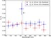 |
Fig. A.1
Comparison of results of the measured Rp/Rs around the potassium doublet using different threshold levels to remove bad pixels and cosmic rays, and no seeing correction in the light curve fitting process. A lower threshold level could produce a spurious detection of an excess in the planet-to-star radius ratio near a deep telluric line as shown by blue squares. The blue and red data points do not present the trend in decreasing Rp/Rs between 750 nm and 870 nm as unlike the results shown in Figs. 9 and 10. |
| Open with DEXTER | |
 |
Fig. A.2
Correlation plot showing the posterior distribution of the parameters fitted to the white light curve of WASP-43b. |
| Open with DEXTER | |
Appendix A.2: Data analysis
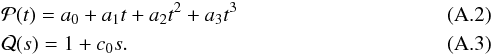
As we explained in Sect. 3.3, we fitted a transit model adding two polynomials to take into account the time and seeing dependent systematic effects present in the data,  (A.1)where
  is a synthetic transit model dependent on the transit parameters VT. For the white light curve VT = (Rp/Rs,u1,u2,Tc,a/Rs,i) with Rp/Rs the planet-to-star radius ratio, (u1,u2) the quadratic limb darkening coefficients, Tc the central time of the transit, a/Rs the semi-major axis over stellar radius, and i the orbital inclination;
  is a time-dependent polynomial, and
  a seeing dependent polynomial:
For the MCMC fitting procedure we followed a similar approach as Berta et al. (2012) and used as likelihood ℒ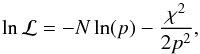 (A.4)where N is the number of points in the curve and p a coefficient to normalize the χ2. The function χ2 compares the data points with the model
 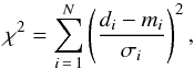 (A.5)where di is the data point, mi the model point, and σi the error in the measurement which in our case was assumed to be the SDNR of the points outside the transit.
The probability priors used for each parameter are presented in Table A.1. The use of a normal prior for the polynomial parameters to take into account the systematic effects was adopted using the information of the MCMC analysis performed using the points outside the transit.
Type of probability priors used in the analysis.
Figure A.2 presents a correlation plot for the posterior distribution of all the parameters used to fit the white light curve. The parameters that are more correlated with the planet-to-star radius ratio are the limb darkening coefficient u2, the semi-major axis over stellar radius a/Rs, and the orbital inclination i.
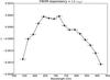 |
Fig. A.3
Seeing coefficient c0 as function of wavelength. The flux losses produced by seeing variations were stronger at both the blue and red ends of the detector. |
| Open with DEXTER | |
Figure A.3 shows the variation of the coefficient c0 used to fit the seeing variations according to Eq. (A.3). The coefficient
varies across wavelength, with a greater dependency on FWHM at both ends of the wavelength range of the detector.
Appendix A.3: Red noise analysis
To compare our error estimation with TAP (Gazak et al. 2012), we performed an analysis of the residuals of the fitted light curves using our MCMC method. The TAP method is based on the paper of Carter & Winn (2009) and computes the red noise contribution in the light curves. Their method is applied when the square of the Fourier transform of the residuals ( ) follow a power law
  (A.6)with A a constant, f the Fourier frequency, and γ the exponent of the power law. If γ = 0 we are in the presence of white noise; if γ = 1.0, pink noise; and if γ = 2.0, red noise.
We computed for the white light curve (see Fig. A.4) and the curves produced using the filters of 75 nm and 25 nm in width. In all the cases the residuals followed a power law with γ ≲ 0.3, indicating that with our fitting procedure the residuals are dominated by white noise. We can also conclude that this γ ≲ 0.3 regime is far from the assumed noise level of TAP (with γ = 1.0), meaning that in this particular case TAP could be overestimating the uncertainties. Since our fitting procedure is close to the white noise regime, we think that our estimation is more accurate than using TAP for this specific data set.
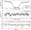 |
Fig. A.4
Red noise analysis. Top panel: white light curve of WASP-43b and best fit. Middle panel: residuals of the white light curve (curve after subtracting the best fit). Bottom panel: square of the Fourier transform of the residuals. A fit of the form A/fγ yields an exponent value of γ = 0.302; according to Carter & Winn (2009) this means that the major noise source in this curve is white noise. |
| Open with DEXTER | |
© ESO, 2014
Current usage metrics show cumulative count of Article Views (full-text article views including HTML views, PDF and ePub downloads, according to the available data) and Abstracts Views on Vision4Press platform.
Data correspond to usage on the plateform after 2015. The current usage metrics is available 48-96 hours after online publication and is updated daily on week days.
Initial download of the metrics may take a while.