| Issue |
A&A
Volume 563, March 2014
|
|
|---|---|---|
| Article Number | A103 | |
| Number of page(s) | 12 | |
| Section | Planets and planetary systems | |
| DOI | https://doi.org/10.1051/0004-6361/201321039 | |
| Published online | 17 March 2014 | |
Constraining physics of very hot super-Earths with the James Webb Telescope. The case of CoRot-7b
1 LESIA, UMR 8109 CNRS, Observatoire de Paris, UVSQ, Université Paris-Diderot, 5 place J. Janssen, 92195 Meudon, France
e-mail: benjamin.samuel@obspm.fr
2 Laboratoire de Météorologie Dynamique, Université Paris 6, Paris, France
3 IAS, CNRS (UMR 8617), Université Paris-Sud, Orsay, France
4 LUTH, Observatoire de Paris, CNRS, Université Paris Diderot, 5 place Jules Janssen, 92190 Meudon, France
5 Canadian Institute for Theoretical Astrophysics, University of Toronto, 60 St Georges Street, Toronto ON M5S 3H8, Canada
Received: 3 January 2013
Accepted: 18 December 2013
Context. Transit detection from space using ultra-precise photometry led to the first detection of super-Earths with solid surfaces: CoRot-7b and Kepler-10b. Because they lie only a few stellar radii from their host stars, these two rocky planets are expected to be extremely hot.
Aims. Assuming that these planets are in a synchronous rotation state and receive strong stellar winds and fluxes, previous studies have suggested that they must be atmosphere-free and that a lava ocean is present on their hot dayside. In this article, we use several dedicated thermal models of the irradiated planet to study how observations with NIRSPEC on the James Webb Space Telescope (JWST) could further confirm and constrain, or reject the atmosphere-free lava ocean planet model for very hot super-Earths.
Methods. Using CoRoT-7b as a working case, we explore the consequences on the phase-curve of a non tidal-locked rotation, with the presence/absence of an atmosphere, and for different values of the surface albedo. We then simulate future observations of the reflected light and thermal emission from CoRoT-7b with NIRSPEC-JWST and look for detectable signatures, such as time lag, of those peculiarities. We also study the possibility to retrieve the latitudinal surface temperature distribution from the observed SED.
Results. We demonstrate that we should be able to constrain several parameters after observations of two orbits (42 h) thanks to the broad range of wavelengths accessible with JWST: i) the Bond albedo is retrieved to within ±0.03 in most cases. ii) The lag effect allows us to retrieve the rotation period within 3 h of a non phase-locked planet, whose rotation would be half the orbital period; for longer period, the accuracy is reduced. iii) Any spin period shorter than a limit in the range 30–800 h, depending on the thickness of the thermal layer in the soil, would be detected. iv) The presence of a thick gray atmosphere with a pressure of one bar, and a specific opacity higher than 10-5 m-2 kg-1 is detectable. v) With spectra up to 4.5 μm, the latitudinal temperature profile can be retrieved to within 30 K with a risk of a totally wrong solution in 5% of the cases. This last result is obtained for a signal-to-noise ratio around 5 per resel, which should be reached on Corot-7 after a total exposure time of ~70 h with NIRSPEC and only three hours on a V = 8 star.
Conclusions. We conclude that it should thus be possible to distinguish the reference situation of a lava ocean with phase-locking and no atmosphere from other cases. In addition, obtaining the surface temperature map and the albedo brings important constraints on the nature or the physical state of the soil of hot super-Earths.
Key words: planets and satellites: atmospheres / planet-star interactions / planets and satellites: physical evolution / planets and satellites: fundamental parameters / planets and satellites: composition / planets and satellites: surfaces
© ESO, 2014
1. Introduction
During the last decade, the development of high precision photometry, particularly from space, led to one of the most exciting, albeit expected, accomplishment: the first detection of massive rocky planets, or the so-called super-Earths (SE). Despite their large masses, the terrestrial nature of these super-Earths has been confirmed by the measure of their mean densities by combining both transit and radial velocity observations. Surprisingly, the first two objects that are observed compatible with a rocky composition, CoRoT-7b (Léger et al. 2009; Queloz et al. 2009; Hatzes et al. 2011) and Kepler-10b (Batalha et al. 2011), appear to be similar in radius (1.68 ± 0.09 and 1.42 ± 0.03 R⊕), mass (7.42 ± 1.21 and 4.56 ± 1.2 M⊕), and environment (they both orbit around a main sequence G star with a very short period roughly equal to 0.85 day). However, their formation is far from being understood. In particular, whether they could have formed in situ or should have migrated to this close orbit or whether they formed as rocky planets or as gas giants whose gaseous envelope subsequently evaporated (Leitzinger et al. 2011) remains unclear.
Considering the magnitude of the energy dissipation induced by the unusually strong tides, this kind of rocky objects should most likely be phase-locked in a very short timescale (<1 My). Furthermore, the extreme UV fluxes and stellar winds received by the planet ensure an efficient atmospheric escape. As a result, if an atmosphere is present, it is probably very thin and in condensation/sublimation equilibrium with the molten surface, although the maximum possible pressure of such an atmosphere is still debated (Schaefer & Fegley 2009; Léger et al. 2011, hereafter L11; Castan & Menou 2011; Kite et al. 2011).
Different parameters used for each model.
According to L11, Mura et al. (2011), and Rouan et al. (2011), the direct expected consequences on the planet surface properties are as follow:
-
A violent thermal gradient between the day/night hemispheres(2500–3000 K versus 50 K)because of the absence of thermal surface redistribution.
-
A large lava ocean on the day side, where the temperature exceeds the rock fusion temperature.
-
A cometary-like tail trailing the planet (Mura et al. 2011). These tails have already been detected for Mercury (e.g. Potter et al. 2002) and possibly for HD 209458 b (Vidal-Madjar et al. 2003). Depending on the atmospheric molecular composition, this tail can be observable. Constraints on the molecules present in the atmosphere of exoplanets have already been inferred from observations with the VLT (Guenther et al. 2011).
To get a better understanding of the extreme nature of this new class of objects, we need more observations. In particular, estimations of the albedo and of the surface fraction occupied by the lava ocean could constrain the composition and the structure of the crust of the planet. The challenging point lies in the difficulty of the direct observation of the emitted/reflected light from these objects because of their very small radius and of the extremely high contrast with respect to the star they orbit. However, Rouan et al. (2011) and Samuel (2011) have shown, respectively, on the example of Kepler-10b and CoRoT-7b, that the modulation of the planetary emitted flux due to the phase effect should be detectable in a near future with the James Webb Space Telescope (JWST). With that in mind, we decided to explore the variety of phase curves that an observer based in the Earth neighborhood would see during the orbit of the considered SE in different physical situations. We decided to focus on the case of CoRoT-7b as a typical example of a very hot SE around a sun-like star. One could easily extend this study with the same method to any other very hot SE, while adapting the properties of the system as the star and the planetary radia, their masses, the magnitude of the star, the orbital period, and so on.
2. Goal
In this article, our goal is thus to estimate how precisely future observations could help to constrain the physical properties of the surface and atmosphere of very hot SE. More specifically, we question the possibility of exploiting the reflection/thermal emission phase curves of very hot SE if they are taken with the accuracy that is anticipated for the JWST. Indeed, this space observatory will be equipped with the largest telescope ever launched in space (6.5 m diameter) and will have, among its various instruments, a near-infrared (IR) spectrometer (NIRSpec) with a 0.6–5 μm spectral range that fits very well with this kind of observations.
In particular, we adress in Sects. 5.1–5.3 the three following problems:
-
How precisely can we infer the surface albedo of the planet? Canwe distinguish a synchronously rotating planet (as expected)from a more rapidly rotating one? Can we estimate the rotationperiod of the planet?
-
Can we infer the presence of an atmosphere, and what is the minimum detectable surface pressure?
-
Can we infer the planetary temperature map by inverting a low resolution spectrum obtain with NIRSpec on JWST?
The range of parameters visited for this study is summarized in the Table 1. To avoid having too many free parameters, we consider CoRoT-7b as a prototype hot SE and carry on the analysis in this study case only. Furthermore, we focus on broadband photometry, so the composition of the rock (Hu et al. 2012) or the observation of molecules in a cometary tail, which requires high spectral resolution, is not examined.
3. Physics and models
In this section, we describe the various physical processes that we have taken into account in the physical model of the planet. Because it is based on simple and conservative assumptions, we consider the Léger et al. (2011) model of an atmosphere-free, tidally-locked planet as being the reference model, and we start by describing its properties in more detail. Then, we discuss the consequences of relaxing some of these constraints.
3.1. The fiducial model: phase-locked, low albedo, atmosphere-free, and lava ocean model
As described in L11, when the planet is tidally locked and has no atmosphere, the surface temperature is in thermal equilibrium and is given at each position (defined by its zenithal angle θ) by 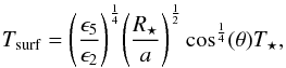 (1)where R⋆ and a are the radius of the SE and the star-planet distance, respectively. The ϵ5 and ϵ2 are the emissivities of the planetary surface in the wavelength range of a black body emission at (resp.) 5250 K and 2200 K. If we assume these two values to be very close (ϵ2 = ϵ5 ≡ ϵ; L11), which is equivalent to assuming that the albedo, A = 1 − ϵ, is constant over the whole visible/IR wavelength range, Tsurf is independent of the albedo of the planet ground.The study of L11 showed that such a situation would lead to a large lava ocean, which is mainly composed of alumina: the most volatile chemicals species must have evaporated and re-condensed over the ocean shores. Assuming an alumina ocean composition, we can derive the extension of the liquid-lava ocean with the shore that corresponds to the melting temperature isotherm.
Now, if we assign any value to ϵ2 = ϵ5 ≡ ϵ ≡ 1 − A, we can derive the planet to star flux ratio at any wavelength and any time along CoRoT-7b orbit. Based on the measurement of Earth lava, L11 assumes a low albedo on CoRoT-7b, but it is a surprise that Kepler-10b seems to show an unexpectedly high Bond albedo of about 0.5 (Batalha et al. 2011; Rouan et al. 2011). The visible light from the host star is more efficiently reflected, but on the other hand, the thermal emission must be less intense, as the albedo is the complementary of the emissivity. If we measure these two effects by observing the phase curve at different wavelengths, we must be able to estimate the albedo value.
3.2. Non synchronous rotation
Although tidal locking is the equilibrium rotation that is reached by a fluid object subjected to tidal dissipation on a circular orbit (Hut 1980), many physical processes can lead to a non synchronous rotation, even when tidal friction is strong. For instance, if a third body in the system (i.e. CoRoT-7c for example) is close and/or massive enough to perturb CoRoT-7b orbit, the planet may not be in a perfectly circularized orbit, which could result in a pseudo-synchronous (faster) planetary rotation. Furthermore, if the solid planet exhibits a permanent asymmetry, it could also be trapped in a spin orbit resonance like Mercury, especially if some eccentricity is present (Makarov et al. 2012). We only consider a coplanar spin-orbit in all this situations.
When this non synchronous rotation is considered, we use the duration of the day as a parameter to define it. This is the exact analog to the solar day that lasts 24 h on Earth. In the following, we use the “day” to quantify the rotation of the planet, because it is the important time scale for an irradiated point at the surface of the planet. When we use the expression rotation period, we refer to the day duration.
To model the temperature map, we need to take into account the thermal inertia of the ground. For the sake of simplicity, this is done by assuming that diffusion is efficient only within an inertia layer of limited depth where temperature is homogeneous. In principle, the thickness of this inertia layer depends on the rotation speed of the planet. As in any diffusion phenomenon, one can assume that the depth of the heat penetration must be proportional to the square root of the heating duration. As the day is shorter (insolated time), then the thinner the rocky inertia layer will be. If we consider of a rocky material with a diffusivity D ~ 1.2 × 10⁻⁶ m2 s-1) and heating with the periodicity P, we can estimate the heat penetration depth by 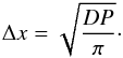 (2)However, to not mix the effect of the depth of the inertia layer with the effect of the rotation period, we prefer to estimate directly the inertia layer size. For a typical day of 20.5 h (the orbital period of CoRoT-7b), we derive a depth of about 15 cm. Thus, we consider the three following heat penetration depths: 2.5 cm, 25 cm, and 2.5 m. This covers the expected range for this parameter, while covering the case of materials with much higher/lower diffusivities. Once this depth is chosen, the thermal inertia of the layer is parametrized by the specific heat of rock (which we assume to depend linearly on the logarithm of the temperature from ~50 to ~2 × 10³ J Kg-1 K-1 from 70–2500 K; Adkins 1983). A more precise estimation of the thermal structure of the floor would necessitate a particular study which is out of the scope of this work.
When the temperature reaches the liquefaction/solidification threshold, it is held fixed until the whole material in the inertia layer is molten/solidified. The latent heat used for this transition is 4 × 10⁵ J kg-1. The duration to melt/solidify the inertia layer depends on the latent heat, the intensity of the incoming stellar flux, and the thickness of the rocky layer.
 |
Fig. 1 Temperature variation at different latitudes of a non phase-locked CoRoT-7b, with a hypothetical day of 10.2 h (half the orbital period of the planet). As the planet is rotating, we can use the time or the longitude on the abscissa. Here, the zero on the time axis corresponds to noon. Each curve represents the temperature at a given latitude (from 0 to 85, with a step of 5°). The plateau at Tfusion = 2300 K is due to the extra energy needed to overpass the latent heat at the threshold of the melting temperature. We can interpret this graph like this for a point which is at low latitude: the rock melts around 1.5 h before noon and so the lava ocean appears; it fully goes back to solid state more than 2 h after noon. The extension of the lava ocean is ± 60° in latitude. |
3.3. Atmospheric redistribution
A dense atmosphere can dramatically change the temperature map of the planet. For example, the temperature difference between the day side and the night side is almost 10 K on Venus and on the Earth, it is 300 K on the Moon or 600 K on Mercury! In the case of very hot SE, the presence of a dense global atmosphere would lead to the redistribution of the heat by advection motion of the gas: the temperature contrast of a few thousands of Kelvin which is expected in the Leger et al. model, could be strongly reduced. Of course, such a scenario would requires us to explain how an atmosphere can survive the combination of a strong wind and of an extremely intense UV field, but this cannot be totally excluded.
Our simulations of a planet with atmosphere have been performed using the LMD generic global climate Model (GCM) specifically developed for the study of extrasolar planets (Wordsworth et al. 2010, 2011; Leconte et al. 2013) and paleoclimates (Wordsworth et al. 2013; Forget et al. 2013). The model uses the 3D dynamical core of the LMDZ 3 GCM (Hourdin et al. 2006), which is based on a finite-difference formulation of the classical primitive equations of meteorology. A spatial resolution of 64 × 64 × 20 in longitude, latitude, and altitude was used for the simulations.
Because the composition and mass of the putative atmosphere remains mostly unconstrained to date, we use a very simple approach and consider only a gray gas. This simple approach is further supported because spectroscopy of complex molecules is poorly known for the high temperatures reached on CoRoT-7b. Considering that our purpose is to see whether or not the atmosphere’s impact on the phase curve would betray its presence, this case is conservative, since, as shown by Selsis et al. (2011), any molecular spectral feature in the spectrum would more easily reveal the atmosphere.
Once a unique specific opacity (κ in m2/kg) has been chosen1 and we have defined the bands in which the flux is computed2, the model uses the same two-stream algorithm developed by Toon et al. (1989) to solve the plane parallel Schwarzschild equation of radiative transfer in previous studies. Thanks to the linearity of the radiative transfer equation, the contribution of the thermal emission and downwelling stellar radiation can be treated separately, even in the same spectral channel. Thermal emission is treated with the hemispheric mean approximation and absorption of the downwelling stellar radiation is treated with collimated beam approximation.
With respect to the other physical parameters, we consider an highly idealized case. We do not account for any condensible species in the atmosphere and, accordingly, do not consider any radiatively active aerosols. The surface is considered flat with a constant albedo of A = 1 − ϵ = 0.3. Turbulent coupling with the surface in the planetary boundary layer is handled by using the parametrization of Mellor & Yamada (1982) and convective adjustement is performed whenever the atmosphere is found to be buoyantly unstable.
Given these assumption, and that planetary parameters are known, we are left with only two free parameters: namely, the specific gas opacity (κ) and the atmospheric column mass (m) or, equivalently, the atmosphere normal optical depth (τ) and the mean surface pressure (ps). Basically, these quantities are linked through  (3)and
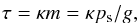 (4)where g is the gravity. Once these parameters are chosen, the model is run from a uniform state at rest until an equilibrium is reached in a statistical sense. Emission maps produced by the GCM are then processed by the tool described in the previous sections to simulate the phase curve and quantify the difference with atmosphere-free planet case.
4. From the model to the simulation of observations
4.1. Phase curve model and simulation of observations with JWST
From the temperature maps computed from the aforementioned model, we can derive the expected phase curve that an observer would measure from the vicinity of the Earth by integrating outgoing flux over the visible hemisphere. The expected planetary flux is the sum of the blackbody emission and the reflected light.
We consider several wavelengths, chosen to optimize the signal-to-noise ratio (S/N) of a supposed observation with the spectrograph NIRSpec on the JWST. The choice of this instrument allows us to investigate a large spectral range (0.6 to 5 μm) from the red, which is useful for characterizing the reflected light to the mid IR, where the thermal emission dominates. The spectral range is divided into five channels which is given in Table 2 (obtained by binning properly the spectrum) and allows us to study the phase curves as a function of the wavelength (Fig. 3).
Then, we use the exposure time calculator3 (Sosey et al. 2012) online tool for estimating the uncertainties on the modeled measurement (instrumental and photon noise); we chose an exposure duration of 72 s, which gives us a good timing for both the phase variations at the different wavelengths, and for the detection of the primary and secondary transits. The transits signature is modeled using the depth from by Léger et al. (2009). As we want to exploit the most precise phase-curve variations, we need at least one whole orbital period (20 h 30 min for CoRoT-7b) of observation. We simulate 41 h of continuous observation of the CoRoT-7 system (2 orbital period of the SE). In such conditions, the peak-to-peak amplitude of the phase curve is the most significant information for the observer and makes the estimation of the global albedo possible (Sect. 5.1.1). Figure 5 shows typical light-curves obtained by this method. A precise analysis of these phase-curve temporal variations is a more delicate task but can provide valuable information on the rotation of the planet and/or the surface temperature map (Sects. 5.1.2 and 5.3).
Note that the secondary transit depth match directly to the peak-to-peak amplitude of the phase curve variations because both the reflected light and the planet thermal emission are masked when the star hides the planet, except if the thermal emission of the night side of the planet is not negligible, in which the secondary transit can appear deeper than the phase curve amplitude value.
4.2. Inverse problem
To quantify the information contained in the light-curves, we used a simple method to explore the simulated data: we fit a modeled light-curve to the data and try to minimize a χ2 function, while browsing the whole parameter space considered (for example, the albedo-day duration space, when we explore the possibility of a non phase-locked situation). We then compare the best couple of parameters obtained with this method with the ones used to produce the simulated data set. We derive the uncertainties directly from the χ2 map (e.g. Fig. 6).
Finally, we try to answer the question: is this observed light-curve compatible with the phase-locked airless planet model? To that purpose, we compute the χ2 difference between the two curves as an estimator of the likelihood. We can then give a simple answer: the simulated situation is either distinguishable or not from the L11’s one.
The global results are presented in the following, as well as few specific exemples to illustrate our discussion.
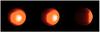 |
Fig. 2 Example of the thermal emission map of a non phase-locked SE at three consecutive values of the orbital phase. The asymmetry in longitude translates the thermal inertia of the ground, partly due to the latent heat when the melting of the rock occurs. |
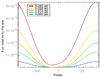 |
Fig. 3 Phase curves in different spectral bands for a non phase-locked CoRoT-7b with a hypothetical day of 10.2 h and an albedo of 0.1. From purple to red, wavelengths of resp. 0.8 μm, 1.125 μm, 1.375 μm, 1.75 μm, and 3.5 μm. The amplitude has been normalized by the stellar flux. As expected (II.4), the phase curve at a longer wavelength shows a clear delay with respect to the one at the shortest wavelength. The zero on the phase axis corresponds to the secondary transit (the observer-star-planet are aligned in this order). The transit and secondary transit signals are not modeled on this figure. |
5. Results
5.1. Retrieval of albedo and rotation
In this subsection, we consider only the airless case and focus on the quantification of the constraints put by light curves on the (albedo, rotation period) couple. To that purpose, we simulated noisy light curves for different values of the albedo and rotation period. For each given noisy light curve, we then mapped the value of χ2 for the whole (albedo, rotation period) parameter space. Examples of such χ2 maps are shown in Figs. 6 and 7. Contours in these maps show us what part of the parameter space can be ruled out for any given confidence level.
We extended this study to different situations with a variable heat penetration depth at the surface: the deeper the heat penetrates the planet crust, the more important the thermal inertia will be. This moderates the temperature variations and lengthen the associated delay. As a result, we see that larger heat penetration depth entails tighter constraints on the rotation period.
5.1.1. Albedo
To focus on the retrieval of the albedo, we first consider only fiducial models with a synchronously locked rotation. An example of a χ2 map for the case with an albedo of 0.3 is shown in Fig. 6. From this map, we can see that the retrieval of the albedo and rotation period is not correlated to each other. We can thus infer a 1σ error bar on the retrieved albedo.
The detailed results are given in Table 3. The albedo corresponding to the maximum confidence level are given for the different simulations. The simulated Bond albedo is allowed to vary from 0.1 to 0.7. We remind that we assume that the albedo is constant with a wavelength in the whole range. A finer hypothesis is discussed in Sect. 5.3. The accuracy on the retrieved albedo is better than 0.05, which is a satisfactory result if we consider that the estimated albedo of the rocky planets is a key factor to get information on the nature of the most superficial layer at the surface. For instance, we should be able to confirm with a much better accuracy the surprising high albedo derived for Kepler-10b (Rouan et al. 2011; Batalha et al. 2011).
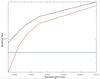 |
Fig. 4 Contribution to the phase curve variation of the reflected light (blue line), thermal emission (red) and total (black). In this example, we took an albedo value of 0.5, so that the reflected flux from the star is higher than the emitted thermal flux from the planet only at wavelengths lower than 1000 nm. |
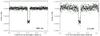 |
Fig. 5 Simulated light curves corresponding to two extreme wavelengths of the observation using JWST-Nirspec. In the left panel, the ideal light-curve (solid green line) expected at 800 nm and the same with the added noise (black cross). The same symbol and color code are used in the right panel for a wavelength of 3.5 μm. |
5.1.2. The planet rotation
When the rotation is not synchronized, the planetary surface receives a variable stellar intensity during the day, and its temperature evolves with time. As on Earth, the maximum temperature does not occur exactly when the star is at its zenith (at noon) but at a short time later: because of its thermal inertia, the ground temperature still increases until the absorbed incoming stellar flux becomes lower than the power lost by thermal emission. Furthermore, if the rock temperature exceeds Tfusion, then the ground will be momentarily melted, and the latent heat will be an additional parameter that changes the thermal inertia. In these conditions, we can get an ephemeral lava ocean that appear and disappear periodically at the same hour everyday, provided that cooling is fast enough, as illustrated in Fig. 1.
Finally, one can notice that a given point of a non phase-locked planet sees its temperature increase as the stellar light intensity increases during the “morning”. Then it cools down during the “afternoon” by emitting radiations (~σT4), but the temperature decreases more and more slowly (as T4 decreases very quickly), making an asymmetric temperature evolution with respect to noon.
A non synchronous planet with a finite thermal inertia thus shows a signature of its rotation in its thermal emission phase curve. The maximum of the IR phase curve does not occur at the same time than for the reflected light. This produces a peculiar signature that would indicate a non synchronized rotation of the planet (see Figs. 2, 3). Since the contrast between the phase-curves (at different wavelength) depends on the albedo, the accuracy of the rotation determination depends on this parameter.
As a result, there is always a rotation period below which the thermal phase curve is too distorted to be confounded with the one of the phase locked planet (to a given confidence level). This lower rotation period (at 1σ) is also given in Table 3. In the case where the thermal inertia is low (heat is exchanged only in the first 2.5 cm of the ground), one cannot differentiate a phase-locked planet from a rotating planet with a 20 h period. On the other hand, the larger (and more realistic) the inertia-layer thickness we use from 25 to 250 cm, the larger this minimum rotation period is. As visible in Fig. 6, (simulated albedo of 0.3 and a thermal exchange thickness of the surface of 2.5 m), we see that we can discriminate a rotating planet with a 200 h period from a phase-locked one with a confidence level of 99%.
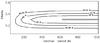 |
Fig. 6 χ2 map showing the compatibility between the observations of a phase-locked CoRoT-7b with a 0.3 Bond albedo and a family of models with various possible albedos and rotation periods, with an inertia-layer thickness of 25 cm. The different contours correspond to the regions where the confidence level for the phase-locked model is 90%, 99%, and 99.99% in the two-parameter space. The gray rectangle corresponds to usual 1σ incertainties (68% confidence level) when we independently study each one of the parameters, while the other is kept constant. |
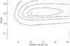 |
Fig. 7 χ2 map comparing a simulated observation of a rotating CoRoT-7b with a 0.3 Bond albedo to a family of models with various albedos, rotation periods, and an inertia-layer thickness of 25 cm. The cross is at the location of the best fitted model in the albedo–period space, and the star marks the position of the initial model (albedo =0.3 and rotation period =10.25 h =1/2 orbital period of CoRoT-7b). |
It can also be noted that we can see a clear correlation between the admissible range of rotation period and the albedo, even if the albedo value is always well constrained: for the lowest Bond albedo values, a larger range of rotation period is excluded. For a 250 cm inertia-layer thickness, an albedo of 0.1 allows us to exclude the rotating planet scenario for a period lower than 840 h (i.e. almost 42 orbital periods of CoRoT-7b). In the same conditions with an albedo of 0.5, this limit is nearly 550 h (27 orbital periods). Finally, we notice a few outliers in these results that do not follow these global trends. This is probably due to statistical deviations in the random noise sample of our simulations, since each result corresponds to one single simulation.
Going further, we tried to quantify the accuracy with which the rotation period of a non synchronous planet could be retrieved from the light curve. Table 1 shows the rotation period limits below which we can significantly distinguish a rotating planet from a phase-locked one. We can deduce that we would be able to estimate a most probable value for the day duration, if the observed planet was showing a short rotation period, which is a day duration shorter than those limits.
Simulated observations with NIRSpec of a phase-locked CoRoT-7b, followed by a phase-curve fitting.
Again, we clearly find that the thickness of the inertia layer strongly influences the ability to retrieve the rotation period. We also notice that the more the phase-curve is singular as the planet rotates upon itself faster and the easier the determination of the period is. In very favorable cases (low albedo, short rotation period and large inertia layer thickness), we can precisely constrain the rotation period and the albedo of the simulated planet. An example of such a case is given in Fig. 7. The albedo is 0.3, the rotation period (day) is 10.25 h long (1/2 orbital period) and the heat penetration depth is 2.5 m. The best fit gives a Bond albedo of  and a rotation period of
  h. In this particular case, it would be easy to precisely deduce the rotation period of the planet and the albedo; the phase-locked scenario could be rejected with a confidence level of 13σ.
Note that we did not consider a high global temperature of the planet, as the possible mechanism we propose to explain a non phase-locked planet should imply4. If it was the case, this could allow us to observe even more easily a potential signature of this situation, with a secondary transit significantly deeper than the phase-curves peak-to-peak amplitude, due to a lower day-night thermal contrast. In this state of mind, Selsis et al. (2013) have recently explored the effect of the tidal heating on the light curves in more tricky situations, such as excentric orbits, spin-orbit resonances, and planets in pseudo-synchronized rotation.
5.2. Atmospheric signature
We now try to assess the possibility of detecting the presence of an atmosphere from the analysis of the phase curves. To avoid mixing different effects, we consider only the phase-locked case. While the presence of a significant atmosphere of silicates in equilibrium with the magma does not seem to be favored (L11), one cannot totally rule out yet the possibility of a non condensable gas being released by the magma ocean, or created by photochemical processes (Schaefer & Fegley 2009; Castan & Menou 2011). For example, the presence of gaseous N2 is not thermodynamically impossible on the day side but also on the night side since the triple point is around 63 K and 13 kPa, when we expect a temperature between 50 K and 75 K in the coldest region (even without atmospheric redistribution). If the flux of the non condensable species released by the different processes can compensate the atmospheric escape, we would be in presence of an atmosphere in an out of equilibrium but steady state situation. In any event, it is worth trying to quantify the constraints on the presence of a potential atmosphere that could be put by observations of phase curves, from an observational point of view.
5.2.1. Simulations
In a first set of simulations, we ran the model for surface pressures of 10 mbar, 100 mbar, and 1bar and kept κ constant to have an optical depth of 10-3, 10-2, and 10-1 respectively. This represents an optically thin case. As expected, the principal effect of the atmosphere is to smooth the initial surface temperature contrasts between the two hemispheres of the planet. At high altitude, hot air is transported from the day to the night side where it can radiate some of its thermal energy.
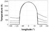 |
Fig. 8 Temperature at the equator of CoRoT-7b in the atmosphere-free case (solid black) compared to the 10, 100, and 1000 mb gray atmosphere cases (dotted, dashed, and solid gray curves, respectively). Substellar point is at longitude 0. The east/west asymmetry on the night side is due to the eastward winds at the equator. |
To estimate the impact of this redistribution on the light curve we computed a bolometric redistribution efficiency (η) defined as the ratio of the total luminosity (due to thermal emission) of the night side over the luminosity of the day side. This ratio should be near 0 for the atmosphere-free case and 1 if the emission is isotropic. As can be seen in Fig. 9, the redistribution efficiency has a low value of 0.1% for a 10mb surface pressure but rises up to 8% for a 1b atmosphere in an almost linear fashion. This low redistribution comes from the thermal timescale of the atmosphere that scales as T-3 and can be very short for such heavily irradiated planet as CoRoT-7b. Simulations of planets receiving a less intense insolation are indeed found to have a higher redistribution efficiency (Leconte et al., in prep.).
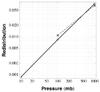 |
Fig. 9 Bolometric redistribution efficiency factor as a function of pressure computed as the luminosity of the night side over the luminosity of the day side for the thin case (κ = 1.5 × 10⁻⁵; solid black curve). For comparison, redistribution in the thicker case is shown (κ = 1.5 × 10⁻², yielding an optical depth of 10 for the 1bar case; dashed gray curve). |
We tested the impact of the optical depth at fixed surface pressure by changing the opacity. Our results suggest that changing the opacity is only a second order effect when compared to the pressure dependence of the redistribution. This is mainly because we use a completely gray model. Emission arises at the same level as absorption (typically at τ = 1) which is the main driver of the day-night temperature gradients. To first order, this should also be true in the real case because stellar insolation and thermal emission occur nearly in the same spectral regions at the high temperatures reached on the dayside. Therefore upper atmospheric levels are very hot; they have a short radiative timescale and cool efficiently before reaching the night side through transport mechanisms (like winds). As a consequence, the optical depth does not directly affect the heat redistribution but changes the amplitude of the phase curve: the thermal contrast increase with the opacity of the atmosphere.
Finally, before assessing the detectability of an atmosphere directly from our synthetic light curves, we computed a spectral redistribution as the luminosity of the night side over the luminosity of the day side in each band of the model (where we have added one band to cover the reddest part of the spectrum where low temperatures night side regions emit strongly). This gives us an understanding of which channels carries the strongest atmospheric signature. Figure 10 shows us that this redistribution is much more difficult to observe for wavelength shorter than 5 microns (less than 10% for the 1b case) while the atmosphere can efficiently smooth luminosity contrasts in the far infrared.
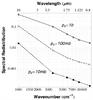 |
Fig. 10 Spectral thermal redistribution efficiency factor as a function of the wavenumber or wavelength,which is computed as the luminosity of the night side over the luminosity of the day side in each band for the thin case (κ = 1.5 × 10⁻⁵). The three different pressures are shown (10 mb: dotted; 100 mb: dashed; 1b: solid). The last band on the left (far IR) is not observable with JWST. |
Taking into account the noise level expected with JWST, we have modeled the effect of the atmosphere on the phase curves and compared it to the atmosphere-free model. The difference becomes significant at a level that crosses the 3σ threshold just below 1 bar when we take κ = 1.5 × 10⁻⁵. If we assume a higher opacity, we find situations more and more favorable from the detection point of view. As shown in Fig. 11, downwelling stellar radiation is more efficiently absorbed and thermalized before reaching the surface when the optical depth increases. As a result, less energy is reflected in the blue part of the spectrum (hence the shallower phase curve in this part of the spectrum) and more is re-emitted thermally in the red part where the planet to star brightness ratio is higher. The atmosphere lowers the bond albedo of the planet when the optical depth is significant, and this amplifies the day-night thermal emission contrast. On the other hand, the heat transport efficiency grows and leads to the warming of the coldest part of the planet surface for higher atmospheric pressures. When opacity and pressure are increasing, this leads to two effects on the amplitude of the phase curves: since both the day and night thermal flux varies in the same direction, the day-night contrast does not change strongly and the phase curves are shifted toward higher value.
In the high pressure and high opacity cases, one can note that, the symmetry of the phase curves is broken, attesting to the effect of (eastward) jets that transport heat, thus offering another signature of the presence of an atmosphere. As a consequence, the observer sees a higher flux from the planet in the interval of time between the transit and the secondary transit (positive phase) than during the period that follows the secondary transit and precedes the primary one (negative phase).
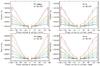 |
Fig. 11 In these graphics, the five dashed lines represent the phase curve expected for a phase-locked atmosphere-free CoRoT-7b with an albedo of 0.3 in the five channels from 0.8 μm (blue) to 3.5 μm (red). The solid lines represent different situations with a grey atmosphere. The relative flux is plotted as a function of the phase, and the zero phase reference is defined as the primary transit position. The parameters for the atmosphere are: top left: P = 100 mb, κ = 1.5 × 10⁻⁵; top right: P = 1b, κ = 1.5 × 10⁻⁵; bottom left: P = 100 mb, κ = 1.5 × 10⁻³; bottom right: P = 1b, κ = 1.5 × 10⁻³. The IR flux from the cold regions is strongly correlated to the pressure, due to the heat transportation by the atmosphere. The opacity plays a role on the flux from the warmer part of the surface: as the atmosphere becomes more opaque, the substellar region becomes warmer; and the thermal flux is higher when these regions are in front of the observer (around phase 180). |
5.2.2. Discussion
In the most favorable situations, we conclude in a positive way on the possibility to distinguish between the presence or the lack of an atmosphere on CoRoT-7b (or on very hot super-Earths in equivalent conditions): if the pressure is about 1 bar or more and the specific opacity is higher than 10-5. The lava ocean model proposed by L11 does not predict such an atmosphere and the JWST should help to confirm this assumption.
What would be the next step to improve the capability to detect the signature of an atmosphere?
First, we did not include any spectral features in the gas absorption spectrum because of the lack of constraints on the atmospheric composition. This is consistent in that thermal emission and stellar radiation spectral domains are almost confounded on the day side. However, the presence of opaque and transparent window regions could directly be seen in the emission spectrum (Selsis et al. 2011). In addition, we note that the stellar light could always heat the lower altitude regions through transparent spectral windows which would allow the upper part of the atmosphere to be cooler and thus to have a more homogeneous horizontal temperature distribution, as explained before. The emission would then be more homogenous in the opaque regions of the spectrum than in the transparent ones (Selsis et al. 2011).
Second, the latter would not only carry sensible but also latent heat if condensable species are present in the atmosphere (silicates for example). As this process can be very efficient even when the amount of condensible gas transported is very small, it could greatly enhance the redistribution efficiency with respect to the one we have calculated. However, considering the lack of constraints on the source and composition of the atmosphere, this issue is beyond the scope of this study.
Even if an atmosphere with a surface pressure between 10 and 100 mb can reach the nightside temperature above the temperature of the freezing point of water, note that these does not mean that such highly irradiated planets are habitable because of the strong positive radiative feedback of water vapor. To really assess the possibility of water stability at the surface, inclusion of the water cycle, as in Leconte et al. (2013), is mandatory.
5.3. Surface temperature distribution.
In the previous sections, we have shown that the future JWST observations will allow us to retrieve global properties of the planet (in particular, albedo and rotation rate) from the light curves. However, we had to assume a specific physical model to infer temperature maps from a given set of these global parameters. In the following section, we relax this assumption, and make an attempt to quantify how the temperature map itself can be retrieved from the observations.
5.3.1. Procedure
To that purpose, we use the following hypotheses:
-
We assume that the photometric data are obtained us-ing the future JWST NIRSPEC instrument with a propersmoothing in the spectral domain so as to synthesizea set of bandpass filters with a given S/N. We used theexposure-time-estimator (ETC) available onthe web for the evaluation of fluxes and noise. In the model, theminimum wavelength and the maximum wavelength are ad-justable and the number of synthesized filters is adjusted so as tohave Δλ/λ = 0.2. We look for the set of parameter values that allow us to retrieve the actual temperature distribution accurately enough at the lowest cost in terms of observing time.
-
Any actual temperature distribution along a meridian (whose polar axis is the star direction) can be described with a fair approximation by T(z), a polynomial expression of fourth degree, with respect to z, the zenith angle of the star direction. This angle is measured from the substellar point and increases toward the terminator. We indeed found that a polynomial expression of fourth degree can fit the radiative equilibrium temperature with an accuracy better than 10-3. If the temperature is redistributed through some other physical processes and tends to be homogeneous, then the polynomial fit should of course still be valid. This assumption reduces the number of free parameters in the fitting procedure to five (the coefficients of the polynomial). We, however, also studied the case where a break in the temperature distribution arises because of the presence of the lava ocean and of a possible difference in the emissivity ratio ϵIR/ϵvis between the lava material and the solid ground.
The procedure we used is as follows. We first model the temperature distribution of the planet assuming that it is phase-locked and that the temperature at its surface is simply the one given by solving the radiative equilibrium equation for a given albedo. Our model for the irradiation takes into account the finite angular extension of the star. The formulation is the one described in Léger et al. (2010). This is the basic temperature distribution we wish to inverse.
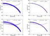 |
Fig. 12 Four examples of temperature distribution retrieval from realistic observations of the planet spectrum using the JWST-NIRSPEC instrument. For each case, 20 trials were done (blue curves). The temperature distribution to be retrieved corresponds to the red curve. The label indicates the conditions in terms of S/N (at the longest wavelength) and of wavelength range. In a few cases, one notes that one or two catastrophic solutions are found. For a S/N = 20 and a wavelength range extending to 4.5 μm, the accuracy on the retrieval of the initial distribution is good (<10 K), and no catastrophic solution is found. |
Then we compute the overall spectrum of the planet as seen from a distant observer. This provides the fluxes in the set of synthetized filters. To assess the importance of the thermal infrared, we have considered two cases, where the overall wavelength range is 0.7–3 μm and 0.7–4.5 μm.
The noise is added according to JWST prescriptions to obtain the desired S/N. Finally, a Powell procedure is used to find the temperature curve, as described by a fourth degree polynomial that produces the best fitting spectrum.
5.3.2. Results
After a few trials, it appeared that the retrieved temperature distribution was often fairly close from the initial one, except for a few cases where the result was catastrophically different. In some cases, for example, the temperature was increasing with solar zenith angle instead of decreasing as it should (see Fig. 12). In general, there is no intermediate situation: a fit is either fairly good (say better than 10 per cent everywhere) or frankly unacceptable (worse than 500 K difference in a significant part of the curve).
We conclude that the requirement on the S/N is finally less based on the accuracy of the retrieved temperature than on the probability to obtain a catastrophic solution for which there is no way to validate it without excluding non physical solutions or by redoing the measurement sequence. We show four examples of temperature inversion for different sets of parameters in Fig. 12, where the S/N and the wavelength range were changed. We give the median error on the retrieved temperature5 and the fraction of catastrophic solution (on 20 trials) for different values of the parameters in Table 4. Even with a medium S/N of 7.5 and provided that the used wavelength range extends up to 4.5 μm, the temperature distribution at the surface of the planet could be retrieved with an accuracy of typically 30 K and a low risk of unreasonable solutions.
Let us now consider the case where the ratio ϵIR/ϵvis differs between the lava surface and the solid ground. We compute the equilibrium temperature by making an additional but physical assumption: the rocky part cannot be hotter than the lava ocean at its bank. Indeed, if (ϵIR/ϵvis)lava > (ϵIR/ϵvis)rock when azimuth is larger than the one of the lava ocean bank, the theoretical equilibrium temperature of the rocky ground would be higher than the melting temperature: in that case, we force it to be at the melting temperature. In doing so, we assume that there is a mix of solid and liquid as long as the rock equilibrium temperature is not below the melting temperature. In Fig. 13, we show two examples where the procedure of retrieving the temperature curve is applied with (ϵIR/ϵvis)lava larger or smaller than (ϵIR/ϵvis)rock. If the retrieved temperature curve is acceptable in the first case, obviously, the break at the bank can hardly be restored by the fourth order polynomial expression in the second case, and the fraction of catastrophic solutions is increased. At this stage, we do not try to go further and use two polynomial expressions one for each medium (lava or rock), but one can easily envision it when necessary.
If we retain that a modest S/N = 5 is sufficient to retrieve the latitudinal temperature profile provided that the wavelength range extends up to 4.5 μm, then we can estimate the time required to obtain it by using the JWST Exposure Time Calculator in the case of Corot-7b (K = 9.8) to be around 70 h. This time could be split in several periods of ~3 h to catch the planet close to to the secondary transit where it offers the largest emitting surface toward the observer. It can be anticipated that future missions (TESS, PLATO) could detect a planet analog to Corot-7b around brighter stars and that the work will be easier in that case. For a G2V star of magnitude K = 6 (V = 8) for instance, the JWST ETC gives an integration time of 9000 s (2.5 h) that would be more easily acceptable given the anticipated competition for observing time.
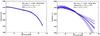 |
Fig. 13 Examples of two situations where (eIR/evis)lava is either larger (left) or smaller (right) than (eIR/evis)rock. The temperature curve is correctly retrieved in the first case while it is clearly not as accurate in the second case where a large fraction (30%) of solutions are of catastrophic type. |
6. Conclusions
In the context of an increasing number of detected very hot super-Earths, such as Corot-7b or Kepler-10b, we have explored whether future observations with the instrument NIRSpec on JWST would allow us to constrain their surface properties. In particular, we have studied how the presence of a dense atmosphere or of a non synchronous rotation of the planet could be inferred from multiwavelength light curves. We also studied to which accuracy one could retrieve the value of the surface Bond albedo and the temperature distribution using the SED between 0.8 and 3.5 μm.
We developed a model of the thermal behavior of the planet surface by assuming that a lava lake is maintained around the substellar point and by considering various cases of heat penetration and albedo. This is done to estimate the time lag of the thermal emission when the planet is not phase-locked and observed all along its orbit. We also modeled the effect of a putative atmosphere at various pressures on the surface temperature using an GCM specifically developed for the study of extrasolar planets. We finally examined how the actual distribution of temperature along a meridian could be retrieved from the observed SED by assuming a polynomial distribution with latitude.
Median error on the temperature for different values of the S/N (from 5 to 20) and for two maximum wavelengths (3 and 4.5 μm).
Thanks to the broad range of wavelengths accessible with JWST and provided that a S/N around 5 per resel is reached after a total exposure time of ~70 h, we are generally able to constrain several of those parameters with a fair accuracy:
-
The Bond albedo is retrieved to within ±0.03 in most cases.
-
Thanks to the asymmetry of the light curve due to the lag effect, the rotation period of a non phase-locked planet is retrieved with an accuracy of 3 h when the rotation is fast, or half the orbital period. For a longer period, the accuracy is reduced.
-
The shortest period compatible with observation of a phase-locked planet is in the range 30–800 h depending on the thickness of the heat penetration layer. This means that any rotation period shorter than this limit would be detectable.
-
We should be able to detect the presence of a gray atmosphere, provided it is thick enough: with a pressure of one bar and an specific opacity higher than 10-5 m-2 kg-1.
-
The latitudinal temperature profile can be retrieved with an accuracy of 10 to 50 K depending on the S/N obtained with NIRSPEC (20 to 5 assumed). We note that the risk of a totally wrong solution is not excluded but is at maximum of 5% for a S/N of 5 and a wavelength range extending to 4.5 μm.
Note that the four first results would still be valid if the exposure time was to be reduced to two complete orbital periods (i.e., 42 h).
These results show that we could test the most current hypothesis of phase-locking and of an atmosphere-free planet for planets similar to Corot-7b and confirm or reject the lava ocean model of L11 by using NIRSPEC-JWST spectra. A precise determination of the albedo and temperature distribution of the planet surface appears also doable, giving the possibility to constrain more precise models of the planet structure and properties. The possible discovery of very hot exolanets around stars brighter than Corot-7 or Kepler-10 would offer better opportunities to test those predictions: for instance, a more affordable integration time of only several hours would be needed for a V = 8 solar-type star.
Of course, one cannot exclude that our model is too simplistic and/or that the effects we did not envision could change some of the conclusions on the feasibility. For instance, the hypothesis concerning a constant albedo, which is independent of wavelength, the nature and the phase (lava or solid) of the soil or, even more so, the hypothesis concerning a gray gas on the atmosphere may seriously affect the amplitude of the time lag effect we predict if the actual situation is significantly different. On the other hand, we consider the two results on the mean abedo derivation and on the possibility to retrieve the latitudinal temperature profile to a large extent as rather solid.
The access to the phase curves simultaneously in visible and near IR seems to be a promising source of information that will provide useful constraints on the very hot super-Earths surfaces and in general on hot exoplanets.
Even a slight non synchronization of the spin-orbit could lead to a global strong warming of the planet and could possibly lead to a fully melted planet (Franck Selsis, priv. comm.). But in this case, once the rock is liquid, the energy dissipation due to the tidal forces should decrease strongly so that the most superficial layer (which radiates the energy flux to space) could then come back to a solid state, forming a crust. The thickness of the crust would be such that an equilibrium of power is reached between some tidal dissipation within the crust, the diffusion of the heat of the melted subsurface and the outward radiation. The important point is that the planet surface could then have a solid surface, and a low tidal dissipation power. We did not conduct a full physical evaluation of this situation, and of course one will have to check if the time constant to return to equilibrium (i.e. phase-locked rotation) is sufficiently long so that there is a chance to observe the transition phase.
References
- Adkins, C. J. 1983, Equilibrium Thermodynamics (Cambridge, UK: Cambridge University Press) [Google Scholar]
- Batalha, N. M., Borucki, W. J., Bryson, S. T., et al. 2011, ApJ, 729, 27 [NASA ADS] [CrossRef] [Google Scholar]
- Castan, T., & Menou, K. 2011, ApJ, 743, L36 [NASA ADS] [CrossRef] [Google Scholar]
- Forget, F., Wordsworth, R., Millour, E., et al. 2013, Icarus, 222, 81 [NASA ADS] [CrossRef] [Google Scholar]
- Guenther, E. W., Cabrera, J., Erikson, A., et al. 2011, A&A, 525, A24 [NASA ADS] [CrossRef] [EDP Sciences] [Google Scholar]
- Hatzes, A. P., Fridlund, M., Nachmani, G., et al. 2011, ApJ, 743, 75 [NASA ADS] [CrossRef] [Google Scholar]
- Hourdin, F., Musat, I., Bony, S., et al. 2006, Climate Dynamics, 27, 787 [Google Scholar]
- Hu, R., Ehlmann, B. L., & Seager, S. 2012, ApJ, 752, 7 [NASA ADS] [CrossRef] [Google Scholar]
- Hut, P. 1980, A&A, 92, 167 [NASA ADS] [Google Scholar]
- Kite, E. S., Gaidos, E., & Manga, M. 2011, ApJ, 743, 41 [NASA ADS] [CrossRef] [Google Scholar]
- Leconte, J., Forget, F., Charnay, B., et al. 2013, A&A, 554, A69 [NASA ADS] [CrossRef] [EDP Sciences] [Google Scholar]
- Léger, A., Rouan, D., Schneider, J., et al. 2009, A&A, 506, 287 [NASA ADS] [CrossRef] [EDP Sciences] [MathSciNet] [Google Scholar]
- Léger, A., Grasset, O., Fegley, B., et al. 2011, Icarus, 213, 1 [NASA ADS] [CrossRef] [Google Scholar]
- Leitzinger, M., Odert, P., Kulikov, Y. N., et al. 2011, Planet. Space Sci., 59, 1472 [NASA ADS] [CrossRef] [Google Scholar]
- Makarov, V. V., Berghea, C., & Efroimsky, M. 2012, ApJ, 761, 83 [NASA ADS] [CrossRef] [Google Scholar]
- Mellor, G. L., & Yamada, T. 1982, Rev. Geophys. Space Phys., 20, 851 [NASA ADS] [CrossRef] [Google Scholar]
- Mura, A., Wurz, P., Schneider, J., et al. 2011, Icarus, 211, 1 [NASA ADS] [CrossRef] [Google Scholar]
- Potter, A. E., Killen, R. M., & Morgan, T. H. 2002, Meteorit. Planet. Sci., 37, 1165 [NASA ADS] [CrossRef] [Google Scholar]
- Queloz, D., Bouchy, F., Moutou, C., et al. 2009, A&A, 506, 303 [NASA ADS] [CrossRef] [EDP Sciences] [Google Scholar]
- Rouan, D., Deeg, H. J., Demangeon, O., et al. 2011, ApJ, 741, L30 [NASA ADS] [CrossRef] [Google Scholar]
- Samuel, B. 2011, Ph.D. Thesis, Université Paris-Sud 11, France [Google Scholar]
- Schaefer, L., & Fegley, B. 2009, ApJ, 703, L113 [NASA ADS] [CrossRef] [Google Scholar]
- Selsis, F., Wordsworth, R. D., & Forget, F. 2011, A&A, 532, A1 [NASA ADS] [CrossRef] [EDP Sciences] [Google Scholar]
- Selsis, F., Maurin, A.-S., Hersant, F., et al. 2013, A&A, 555, A51 [NASA ADS] [CrossRef] [EDP Sciences] [Google Scholar]
- Sosey, M., Hanley, C., Laidler, V., et al. 2012, in Astronomical Data Analysis Software and Systems XXI, eds. P. Ballester, D. Egret, & N. P. F. Lorente, ASP Conf. Ser., 461, 221 [Google Scholar]
- Toon, O. B., McKay, C. P., Ackerman, T. P., & Santhanam, K. 1989, J. Geophys. Res., 94, 16287 [NASA ADS] [CrossRef] [Google Scholar]
- Vidal-Madjar, A., Lecavelier des Etangs, A., Désert, J.-M., et al. 2003, Nature, 422, 143 [NASA ADS] [CrossRef] [PubMed] [Google Scholar]
- Wordsworth, R. D., Forget, F., Selsis, F., et al. 2010, A&A, 522, A22 [NASA ADS] [CrossRef] [EDP Sciences] [Google Scholar]
- Wordsworth, R. D., Forget, F., Selsis, F., et al. 2011, ApJ, 733, L48 [NASA ADS] [CrossRef] [Google Scholar]
- Wordsworth, R., Forget, F., Millour, E., et al. 2013, Icarus, 222, 1 [NASA ADS] [CrossRef] [Google Scholar]
All Tables
Simulated observations with NIRSpec of a phase-locked CoRoT-7b, followed by a phase-curve fitting.
Median error on the temperature for different values of the S/N (from 5 to 20) and for two maximum wavelengths (3 and 4.5 μm).
All Figures
|
Fig. 1 Temperature variation at different latitudes of a non phase-locked CoRoT-7b, with a hypothetical day of 10.2 h (half the orbital period of the planet). As the planet is rotating, we can use the time or the longitude on the abscissa. Here, the zero on the time axis corresponds to noon. Each curve represents the temperature at a given latitude (from 0 to 85, with a step of 5°). The plateau at Tfusion = 2300 K is due to the extra energy needed to overpass the latent heat at the threshold of the melting temperature. We can interpret this graph like this for a point which is at low latitude: the rock melts around 1.5 h before noon and so the lava ocean appears; it fully goes back to solid state more than 2 h after noon. The extension of the lava ocean is ± 60° in latitude. |
| In the text | |
|
Fig. 2 Example of the thermal emission map of a non phase-locked SE at three consecutive values of the orbital phase. The asymmetry in longitude translates the thermal inertia of the ground, partly due to the latent heat when the melting of the rock occurs. |
| In the text | |
|
Fig. 3 Phase curves in different spectral bands for a non phase-locked CoRoT-7b with a hypothetical day of 10.2 h and an albedo of 0.1. From purple to red, wavelengths of resp. 0.8 μm, 1.125 μm, 1.375 μm, 1.75 μm, and 3.5 μm. The amplitude has been normalized by the stellar flux. As expected (II.4), the phase curve at a longer wavelength shows a clear delay with respect to the one at the shortest wavelength. The zero on the phase axis corresponds to the secondary transit (the observer-star-planet are aligned in this order). The transit and secondary transit signals are not modeled on this figure. |
| In the text | |
|
Fig. 4 Contribution to the phase curve variation of the reflected light (blue line), thermal emission (red) and total (black). In this example, we took an albedo value of 0.5, so that the reflected flux from the star is higher than the emitted thermal flux from the planet only at wavelengths lower than 1000 nm. |
| In the text | |
|
Fig. 5 Simulated light curves corresponding to two extreme wavelengths of the observation using JWST-Nirspec. In the left panel, the ideal light-curve (solid green line) expected at 800 nm and the same with the added noise (black cross). The same symbol and color code are used in the right panel for a wavelength of 3.5 μm. |
| In the text | |
|
Fig. 6 χ2 map showing the compatibility between the observations of a phase-locked CoRoT-7b with a 0.3 Bond albedo and a family of models with various possible albedos and rotation periods, with an inertia-layer thickness of 25 cm. The different contours correspond to the regions where the confidence level for the phase-locked model is 90%, 99%, and 99.99% in the two-parameter space. The gray rectangle corresponds to usual 1σ incertainties (68% confidence level) when we independently study each one of the parameters, while the other is kept constant. |
| In the text | |
|
Fig. 7 χ2 map comparing a simulated observation of a rotating CoRoT-7b with a 0.3 Bond albedo to a family of models with various albedos, rotation periods, and an inertia-layer thickness of 25 cm. The cross is at the location of the best fitted model in the albedo–period space, and the star marks the position of the initial model (albedo =0.3 and rotation period =10.25 h =1/2 orbital period of CoRoT-7b). |
| In the text | |
|
Fig. 8 Temperature at the equator of CoRoT-7b in the atmosphere-free case (solid black) compared to the 10, 100, and 1000 mb gray atmosphere cases (dotted, dashed, and solid gray curves, respectively). Substellar point is at longitude 0. The east/west asymmetry on the night side is due to the eastward winds at the equator. |
| In the text | |
|
Fig. 9 Bolometric redistribution efficiency factor as a function of pressure computed as the luminosity of the night side over the luminosity of the day side for the thin case (κ = 1.5 × 10⁻⁵; solid black curve). For comparison, redistribution in the thicker case is shown (κ = 1.5 × 10⁻², yielding an optical depth of 10 for the 1bar case; dashed gray curve). |
| In the text | |
|
Fig. 10 Spectral thermal redistribution efficiency factor as a function of the wavenumber or wavelength,which is computed as the luminosity of the night side over the luminosity of the day side in each band for the thin case (κ = 1.5 × 10⁻⁵). The three different pressures are shown (10 mb: dotted; 100 mb: dashed; 1b: solid). The last band on the left (far IR) is not observable with JWST. |
| In the text | |
|
Fig. 11 In these graphics, the five dashed lines represent the phase curve expected for a phase-locked atmosphere-free CoRoT-7b with an albedo of 0.3 in the five channels from 0.8 μm (blue) to 3.5 μm (red). The solid lines represent different situations with a grey atmosphere. The relative flux is plotted as a function of the phase, and the zero phase reference is defined as the primary transit position. The parameters for the atmosphere are: top left: P = 100 mb, κ = 1.5 × 10⁻⁵; top right: P = 1b, κ = 1.5 × 10⁻⁵; bottom left: P = 100 mb, κ = 1.5 × 10⁻³; bottom right: P = 1b, κ = 1.5 × 10⁻³. The IR flux from the cold regions is strongly correlated to the pressure, due to the heat transportation by the atmosphere. The opacity plays a role on the flux from the warmer part of the surface: as the atmosphere becomes more opaque, the substellar region becomes warmer; and the thermal flux is higher when these regions are in front of the observer (around phase 180). |
| In the text | |
|
Fig. 12 Four examples of temperature distribution retrieval from realistic observations of the planet spectrum using the JWST-NIRSPEC instrument. For each case, 20 trials were done (blue curves). The temperature distribution to be retrieved corresponds to the red curve. The label indicates the conditions in terms of S/N (at the longest wavelength) and of wavelength range. In a few cases, one notes that one or two catastrophic solutions are found. For a S/N = 20 and a wavelength range extending to 4.5 μm, the accuracy on the retrieval of the initial distribution is good (<10 K), and no catastrophic solution is found. |
| In the text | |
|
Fig. 13 Examples of two situations where (eIR/evis)lava is either larger (left) or smaller (right) than (eIR/evis)rock. The temperature curve is correctly retrieved in the first case while it is clearly not as accurate in the second case where a large fraction (30%) of solutions are of catastrophic type. |
| In the text | |
Current usage metrics show cumulative count of Article Views (full-text article views including HTML views, PDF and ePub downloads, according to the available data) and Abstracts Views on Vision4Press platform.
Data correspond to usage on the plateform after 2015. The current usage metrics is available 48-96 hours after online publication and is updated daily on week days.
Initial download of the metrics may take a while.