| Issue |
A&A
Volume 562, February 2014
|
|
|---|---|---|
| Article Number | A91 | |
| Number of page(s) | 16 | |
| Section | Galactic structure, stellar clusters and populations | |
| DOI | https://doi.org/10.1051/0004-6361/201322531 | |
| Published online | 12 February 2014 | |
The RAVE survey: the Galactic escape speed and the mass of the Milky Way
1
Leibniz-Institut für Astrophysik Potsdam (AIP),
An der Sternwarte
16, 14482
Potsdam,
Germany
e-mail:
tilmann.piffl@physics.ox.ac.uk
2
Rudolf Peierls Centre for Theoretical Physics, 1 Keble Road,
Oxford
OX1 3NP,
UK
3
Institute for Astronomy, University of Cambridge,
Madingley Road,
Cambridge
CB3 0HA,
UK
4
Dept. of Astronomy and Astrophysics, Villanova University,
800 E Lancaster
Ave, Villanova,
PA
19085,
USA
5
Observatoire astronomique de Strasbourg, Université de Strasbourg,
CNRS, UMR 7550, 11 rue de l’Université, 67000
Strasbourg,
France
6
Sydney Institute for Astronomy, University of Sydney, School of
Physics A28, NSW,
2088,
Australia
7
Astronomisches Rechen-Institut, Zentrum für Astronomie der
Universität Heidelberg, Mönchhofstr. 12–14, 69120
Heidelberg,
Germany
8
Research School of Astronomy and Astrophysics, Australian National
University, Cotter Rd.,
ACT
2611
Weston,
Australia
9
Jeremiah Horrocks Institute, University of Central Lancashire,
Preston,
PR1 2HE,
UK
10
Kapteyn Astronomical Institute, University of Groningen,
PO Box 800,
9700 AV
Groningen, The
Netherlands
11
National Institute of Astrophysics INAF, Astronomical Observatory
of Padova, 36012
Asiago,
Italy
12
Senior CIfAR Fellow, University of Victoria,
Victoria BC,
V8P 5C2,
Canada
13
Department of Physics, Macquarie University, NSW,
2109
Sydney,
Australia
14
Research Centre for Astronomy, Astrophysics and Astrophotonics,
Macquarie University, NSW,
2109
Sydney,
Australia
15
Australian Astronomical Observatory, PO Box 296,
NSW 1710
Epping,
Australia
16
Mullard Space Science Laboratory, University College London,
Holmbury St Mary,
Dorking, RH5 6NT, UK
17
Australian Astronomical Observatory, PO Box 915,
NSW 1670
North Ryde,
Australia
18
Department of Physics & Astronomy, Johns Hopkins
University, Baltimore, MD
21218,
USA
19
University of Ljubljana, Faculty of Mathematics and Physics,
Jadranska 19,
1000
Ljubljana,
Slovenia
20
Center of excellence space-si, Askerceva 12,
1000
Ljubljana,
Slovenia
Received:
23
August
2013
Accepted:
12
November
2013
We made new estimates of the Galactic escape speed at various Galactocentric radii using the latest data release of the RAdial Velocity Experiment (RAVE DR4). Compared to previous studies we have a database that is larger by a factor of 10, as well as reliable distance estimates for almost all stars. Our analysis is based on statistical analysis of a rigorously selected sample of 90 high-velocity halo stars from RAVE and a previously published data set. We calibrated and extensively tested our method using a suite of cosmological simulations of the formation of Milky Way-sized galaxies. Our best estimate of the local Galactic escape speed, which we define as the minimum speed required to reach three virial radii R340, is 533+54-41 km s-1 (90% confidence), with an additional 4% systematic uncertainty, where R340 is the Galactocentric radius encompassing a mean overdensity of 340 times the critical density for closure in the Universe. From the escape speed we further derived estimates of the mass of the Galaxy using a simple mass model with two options for the mass profile of the dark matter halo: an unaltered and an adiabatically contracted Navarro, Frenk & White (NFW) sphere. If we fix the local circular velocity, the latter profile yields a significantly higher mass than the uncontracted halo, but if we instead use the statistics for halo concentration parameters in large cosmological simulations as a constraint, we find very similar masses for both models. Our best estimate for M340, the mass interiorto R340 (dark matter and baryons), is 1.3+0.4-0.3 × 10¹² M⊙ (corresponds to M200 = 1.6+0.5-0.4 × 10¹² M⊙). This estimate is in good agreement with recently published, independent mass estimates based on the kinematics of more distant halo stars and the satellite galaxy Leo I.
Key words: Galaxy: general / Galaxy: fundamental parameters / Galaxy: kinematics and dynamics / Galaxy: structure / Galaxy: halo
© ESO, 2014
1. Introduction
In recent years quite a large number of studies concerning the mass of our Galaxy have been published. This parameter is of particular interest, because it provides a test of the current cold dark matter paradigm. There is now convincing evidence (e.g., Smith et al. 2007) that the Milky Way (MW) exhibits a similar discrepancy between luminous and dynamical mass estimates as already found in the 1970’s for other galaxies. A robust measurement of this parameter is needed to place the Milky Way in a cosmological framework. Furthermore, detailed knowledge of the mass and the mass profile of the Galaxy is crucial for understanding and modeling the dynamic evolution of the MW satellite galaxies (e.g., Kallivayalil et al. 2013, for the Magellanic clouds) and the Local Group (van der Marel et al. 2012b,a).
Generally, it can be observed that mass estimates based on stellar kinematics yield low values ≲1012 M⊙ (Smith et al. 2007; Xue et al. 2008; Kafle et al. 2012; Deason et al. 2012; Bovy et al. 2012), while methods exploiting the kinematics of satellite galaxies or statistics of large cosmological dark matter simulations find higher values (Wilkinson & Evans 1999; Li & White 2008; Boylan-Kolchin et al. 2011; Busha et al. 2011; Boylan-Kolchin et al. 2013). There are some exceptions, however. For example, Przybilla et al. (2010) find a rather high value of 1.7 × 10¹² M⊙ when taking the star J1539+0239 into account. This is hyper-velocity star approaching the MW. Gnedin et al. (2010) find a similar value using Jeans modeling of a stellar population in the outer halo. On the other hand, Vera-Ciro et al. (2013) estimate a most likely MW mass of 0.8 × 10¹² M⊙ by analyzing the Aquarius simulations (Springel et al. 2008) in combination with semi-analytic models of galaxy formation. Watkins et al. (2010) report an only slightly higher value based on the line-of-sight velocities of satellite galaxies (see also Sales et al. 2007), but when they include proper motion estimates they again find a higher mass of 1.4 × 10¹² M⊙. Using a mixture of stars and satellite galaxies, Battaglia et al. (2005, 2006) also find a low mass below 1012 M⊙. McMillan (2011) find an intermediate mass of 1.3 × 10¹² M⊙, including constraints from photometric data. A further complication comes from the definition of the total mass of the Galaxy which is different for different authors and so a direct comparison of the quoted values has to be made with care. Finally, there is an independent, strong upper limit for the Milky Way mass coming from Local Group timing arguments that estimate the total mass of the combined mass of the Milky Way and Andromeda to 3.2 ± 0.6 × 10¹² M⊙ (van der Marel et al. 2012b).
In this work we attempt to estimate the mass of the MW through measuring the escape speed at several Galactocentric radii. In this we follow up on the studies by Leonard & Tremaine (1990), Kochanek (1996), and Smith et al. (2007, S07, hereafter). The latter work made use of an early version of the RAdial Velocity Experiment (RAVE; Steinmetz et al. 2006), a massive spectroscopic stellar survey that finished its observational phase in April 2013, and the almost complete set of data will soon be publicly available in the fourth data release (Kordopatis et al. 2013). This tremendous data set forms the foundation of our study.
The escape speed measures the depth of the potential well of the Milky Way and therefore
contains information about the mass distribution outside the radius for which it is
estimated. It thus constitutes a local measurement connected to the very outskirts of our
Galaxy. In the absence of dark matter and a purely Newtonian gravity law, we would expect a
local escape speed of  km s-1, assuming the local standard of rest VLSR to
be 220 km s-1 and neglecting the small fraction of visible mass outside the solar
circle (Fich & Tremaine 1991). However, the
estimates in the literature are much greater than this value, starting with a minimum value
of 400 km s-1 (Alexander 1982) to the
currently most precise measurement by S07, who find [498, 608] km s-1 as a 90%
confidence range.
km s-1, assuming the local standard of rest VLSR to
be 220 km s-1 and neglecting the small fraction of visible mass outside the solar
circle (Fich & Tremaine 1991). However, the
estimates in the literature are much greater than this value, starting with a minimum value
of 400 km s-1 (Alexander 1982) to the
currently most precise measurement by S07, who find [498, 608] km s-1 as a 90%
confidence range.
The paper is structured as follows. In Sect. 2 we introduce the basic principles of our analysis. Then we go on (Sect. 3) to describe how we use cosmological simulations to obtain a prior for our maximum likelihood analysis and thereby calibrate our method. After presenting our data and the selection process in Sect. 4, we obtain estimates on the Galactic escape speed in Sect. 5. The results are extensively discussed in Sect. 6, and mass estimates for our Galaxy are obtained and compared to previous measurements. Finally, we conclude and summarize in Sect. 7.
2. Methodology
The basic analysis strategy applied in this study was initially introduced by Leonard & Tremaine (1990) and later extended by
S07. They assumed that the stellar system could be described by an ergodic distribution
function (DF) f(E) that satisfied f → 0
as E → Φ, the local value of the gravitational potential
Φ(r). Then the density of stars in velocity space will be
a function n(ν) of speed ν and tend to zero as
ν→ νesc = (2Φ)1/2. Leonard & Tremaine (1990) proposed that the asymptotic behavior
of n(ν) could be modeled as  (1)for
ν< νesc, where k is a parameter. We
should therefore be able to obtain an estimate of νesc from a local sample of
stellar velocities. S07 used a slightly different functional form,
(1)for
ν< νesc, where k is a parameter. We
should therefore be able to obtain an estimate of νesc from a local sample of
stellar velocities. S07 used a slightly different functional form,  (2)that can be derived if
f(E) ∝ Ek
is assumed, but, as we see in Sect. 3, results from
cosmological simulations are approximated better by Eq. (1).
(2)that can be derived if
f(E) ∝ Ek
is assumed, but, as we see in Sect. 3, results from
cosmological simulations are approximated better by Eq. (1).
Currently, the most accurate velocity measurements are line-of-sight velocities, νlos, obtained from spectroscopy via the Doppler effect. These measurements have typical uncertainties of a few km s-1, which is an order of magnitude smaller than the typical uncertainties on tangential velocities obtained from the proper motions currently available. Leonard & Tremaine (1990) have already showed with simulated data that because of this, estimates from radial velocities alone are as accurate as estimates that use proper motions as well. The measured velocities νlos have to be corrected for the solar motion to enter a Galactocentric rest frame. These corrected velocities we denote with ν∥.
Following Leonard & Tremaine (1990), we can
infer the distribution of ν∥ by integrating over all perpendicular directions:
 (3)again
for | ν∥| < νesc. Here δ
denotes the Dirac delta function and
(3)again
for | ν∥| < νesc. Here δ
denotes the Dirac delta function and  represents a unit vector along the line of sight.
We do not expect that our approximation for the velocity DF is valid over the whole range of velocities, but only at the high velocity tail of the distribution. We therefore impose a lower limit νmin for the stellar velocities. A further important requirement is that the stellar velocities come from a population that is not rotationally supported, because such a population is clearly not described by an ergodic DF. In the case of stars in the Galaxy, this means that we have to select for stars of the Galactic stellar halo component.
We now apply the following approach to the estimation of νesc. We adopt the
likelihood function  (4)and
determine the likelihood of our catalog of stars that have
| ν∥| > νmin for various choices of
νesc and k, then we marginalize the likelihood over the
nuisance parameter k and determine the true value of νesc as the
speed that maximizes the marginalized likelihood.
(4)and
determine the likelihood of our catalog of stars that have
| ν∥| > νmin for various choices of
νesc and k, then we marginalize the likelihood over the
nuisance parameter k and determine the true value of νesc as the
speed that maximizes the marginalized likelihood.
2.1. Non-local modeling
Structural parameters of the baryonic components of our Galaxy model.
Leonard & Tremaine (1990) (and in a similar form also S07) used Eq. (3) and the maximum likelihood method to obtain constraints on νesc and k in the solar neighborhood. This rests on the assumptions that the stars whose velocities are used are confined to a volume that is small compared to the size of the Galaxy and thus that νesc is approximately constant in this volume.
In this study we go a step further and take the individual positions of the stars into
account. We do this in two slightly different ways: (1) one can sort the data into
Galactocentric radial distance bins and analyze them independently. (2) Alternatively, all
velocities in the sample are rescaled to the escape speed at the Sun’s position,
 (5)where
r0 is the position vector of the Sun. For the
gravitational potential, Φ(r), model assumptions have to be
made. This approach makes use of the full capabilities of the maximum likelihood method to
deal with unbinned data and thereby exploit all the information available.
(5)where
r0 is the position vector of the Sun. For the
gravitational potential, Φ(r), model assumptions have to be
made. This approach makes use of the full capabilities of the maximum likelihood method to
deal with unbinned data and thereby exploit all the information available.
We compare the two approaches using the same mass model: a Miyamoto & Nagai (1975) disk and a Hernquist (1990) bulge for the baryonic components, and for the dark matter halo an original or an adiabatically contracted NFW profile (Navarro et al. 1996; Mo et al. 1998). As structural parameters of the disk and the bulge, we use common values that were also used by S07 and Xue et al. (2008) and are given in Table 1. Apart from its virial mass the NFW profile has the (initial) concentration parameter c as a free parameter. In most cases we fix c by requiring the circular speed at the solar radius, νcirc(R0), to be equal to the local standard of rest, VLSR (after a possible contraction of the halo). As a result our simple model only has one free parameter, its virial mass. For our results from the first approach using Galactocentric bins, we alternatively apply a prior for c taken from the literature to reduce our dependence on the somewhat uncertain value of the local standard of rest.
2.2. General behavior of the method
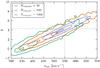 |
Fig. 1 Maximum likelihood parameter pairs computed from mock velocity samples of different sizes. The dotted lines denote the input parameters of the underlying velocity distribution. The contour lines denote positions where the number density fell to 0.9, 0.5, and 0.05 times the maximum value. |
To learn more about the general reliability of our analysis strategy, we created random velocity samples drawn from a distribution according to Eq. (3) with νesc = 550 km s-1 and k = 4.3. For each sample we computed the maximum likelihood values for νesc and k. Figure 1 shows the resulting parameter distributions for three different sample sizes: 30, 100, and 1000 stars. Five thousand samples were created for each value. One immediately recognizes a strong degeneracy between νesc and k, and the method tends to find parameter pairs with too low a escape speed. This behavior is easy to understand if one considers the asymmetric shape of the velocity distribution. The position of the maximum likelihood pair strongly depends on the highest velocity in the sample – if the highest velocity is relatively low, the method will favor too low a escape speed. This demonstrates the need for additional knowledge about the power index k as already noticed by S07.
3. Constraints for k from cosmological simulations
Almost all of the recent estimates of the Milky Way mass have made use of cosmological simulations (e.g., Smith et al. 2007; Xue et al. 2008; Busha et al. 2011; Boylan-Kolchin et al. 2013). In particular, those estimates that rely on stellar kinematics (Smith et al. 2007; Xue et al. 2008) make use of the realistically complex stellar velocity distributions provided by numerical experiments. In this study we also follow this approach. S07 used simulations to show that the velocity distributions indeed reach all the way up to the escape speed, but more importantly, from the simulated stellar kinematics, they derived priors on the power-law index k. This was fundamental for their study on account of the strong degeneracy between k and the escape speed shown in Fig. 1 because there were not enough data to break this degeneracy. As we show later, despite our larger data set, we still face the same problem. However, with the advanced numerical simulations available today, we can do a much more detailed analysis.
In this study we make use of the simulations by Scannapieco et al. (2009). This suite of eight simulations comprises resimulations of the extensively studied Aquarius halos (Springel et al. 2008), including gas particles using a modified version of the Gadget-3 code including star formation, supernova feedback, metal-line cooling, and the chemical evolution of the interstellar medium. The initial conditions for the eight simulations were randomly selected from a dark-matter-only simulation of a much larger volume. The only selection criteria were a final halo mass similar to what is measured for the mass of the Milky Way and no other massive galaxy in the vicinity of the halo at redshift zero. We adopted the naming convention for the simulation runs (A – H) from Scannapieco et al. (2009). The initial conditions of simulation C were also used in the Aquila comparison project (Scannapieco et al. 2012). The galaxies have virial masses between 0.7–1.6 × 10¹² M⊙ and span a wide range of morphologies, from galaxies with a significant disk component (e.g., simulations C and G) to pure elliptical galaxies (simulation F). The mass resolution is 0.22–0.56 × 10⁶ M⊙. For a detailed description of the simulations, we refer the reader to Scannapieco et al. (2009, 2010, 2011). Details regarding the simulation code can be found in Scannapieco et al. (2005, 2006) and also in Springel (2005).
An important aspect of the Scannapieco et al. (2009) sample is that the eight simulated galaxies have a broad variety of merger and accretion histories, thereby providing a more or less representative sample of Milky Way-mass galaxies formed in a ΛCDM universe (Scannapieco et al. 2011). Our set of simulations is thus useful for the present study, since it gives us information on the evolution of various galaxies, including all the necessary cosmological processes acting during the formation of galaxies and at relatively high resolution.
Virial radii, masses, and velocities after rescaling the simulations to have a circular speed of 220 km s-1 at the solar radius R0 = 8.28 kpc.
Also, we note that the same code has been successfully applied to the study of dwarf galaxies (Sawala et al. 2011, 2012), using the same set of input parameters. Despite a mismatch in the baryon fraction (common to almost all simulations of this kind), the resulting galaxies exhibited structures and stellar populations consistent with observations, proving that the code is able to reproduce the formation of galaxies of different masses in a consistent way. Considering that the outer stellar halo of massive galaxies form from smaller accreted galaxies, that we do not need to fine-tune the code differently for different masses once more proves the reliability of the simulation code and its results.
To allow a better comparison to the Milky Way we rescale the simulations to have a circular
speed at the solar radius, R0 = 8.28 kpc, of 220
km s-1 by the following transformation: 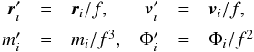 (6)where
mi and Φi are the
mass and the gravitational potential energy of the ith star particle in the
simulations. The resulting masses, M340, radii,
R340, and velocities, V340, as
well as the scaling factors, are given in Table 2.
Throughout this work we use a Hubble constant H = 73
km s-1 Mpc-1 and define the virial radius to contain a mean matter
density 340 ρcrit, where
ρcrit = 3H2/8πG
is the critical energy density for a closed universe1.
The above transformations do not alter the simulation results since they preserve the
numerical value of the gravitational constant G governing the stellar
motions, the mass density field ρ(r) that
governs the gas motions, and the numerical star formation recipe. Only the supernova
feedback recipe does not scale in the same way, but since our scaling factors
f are close to unity, this is not a major concern.
(6)where
mi and Φi are the
mass and the gravitational potential energy of the ith star particle in the
simulations. The resulting masses, M340, radii,
R340, and velocities, V340, as
well as the scaling factors, are given in Table 2.
Throughout this work we use a Hubble constant H = 73
km s-1 Mpc-1 and define the virial radius to contain a mean matter
density 340 ρcrit, where
ρcrit = 3H2/8πG
is the critical energy density for a closed universe1.
The above transformations do not alter the simulation results since they preserve the
numerical value of the gravitational constant G governing the stellar
motions, the mass density field ρ(r) that
governs the gas motions, and the numerical star formation recipe. Only the supernova
feedback recipe does not scale in the same way, but since our scaling factors
f are close to unity, this is not a major concern.
Since the galaxies in the simulations are not isolated systems, we have to define a limiting distance above which we consider a particle to have escaped its host system. We set this distance to 3R340 and set the potential to zero at this radius, which results in distances between 430 and 530 kpc in the simulations. This choice is an educated guess, and our results are not sensitive to small changes, because the gravitational potential changes only weakly with radius at these distances, and in addition, the resulting escape speed is only proportional to the square root of the potential. However, we must not choose too low a value, because otherwise we underestimate the escape speed encoded in the stellar velocity field. On the other hand, we must set the cut-off in a regime where the potential is not yet dominated by neighboring (clusters of) galaxies. Our choice is, in addition, close to half of the distance of the Milky Way and its nearest massive neighbor, the Andromeda galaxy. We test our choice further below. With this definition of the cut-off radius, we obtain local escape speeds at R0 from the center between 475 and 550 km s-1.
Now we select a population of star particles belonging to the stellar halo component. In many numerical studies, the separation of the particles into disk and bulge/halo populations is done using a circularity parameter that is defined as the ratio between the particle’s angular momentum in the z-direction2 and the angular momentum of a circular orbit either at the particle’s current position (Scannapieco et al. 2009, 2011) or at the particle’s orbital energy (Abadi et al. 2003). A threshold value is then defined to divide disk and bulge/halo particles. We opt for the very conservative value of 0, which means that we only take counter-rotating particles. Practically speaking, this is equivalent to selecting all particles with a positive tangential velocity with respect to the Galactic center. This choice allows us to do exactly the same selection as we will do later with the real observational data, for which we have to use a very conservative value because of the larger uncertainties in the proper motion measurements.
For similar reasons, we also keep only particles in our sample that have Galactocentric distances between 4 and 12 kpc, which reflects the range of values of the stars in the RAVE survey that we use for this study. This further ensures that we exclude particles belonging to the bulge component.
Finally, we set the distance R0 of the observer from the Galactic center to be 8.28 kpc, choose an azimuthal position φ0, and compute the line-of-sight velocity ν∥ ,i for each particle in the sample. We furthermore know the exact potential energy Φi of each particle and therefore their local escape speed νesc,i is easily computed.
We do this for four different azimuthal positions separated from each other by 90°. The positions were chosen such that the inclination angle with respect to a possible bar is 45°. The corresponding samples are analyzed individually and also combined. These samples are practically statistically independent even though a particle could enter two or more samples. However, because we restrict ourselves the line-of-sight component of the velocities, only in the unlikely case that a particle is located exactly on the line-of-sight between two observer positions, it would gain an incorrect double weight in the combined statistical analysis.
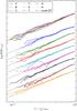 |
Fig. 2 Normalized velocity distributions of the stellar halo population in our eight simulations plotted as a function of 1−ν∥/νesc. Only counter-rotating particles that have Galactocentric distances r between 4 and 12 kpc are considered to select for halo particles (see Sect. 3.1) and to match the volume observed by the RAVE survey. To allow a comparison, each velocity was divided by the escape speed at the particle’s position. Different colors indicate different simulations, and for each simulation the ν∥ distribution is shown for four different observer positions. The top bundle of curves shows the mean of these four distributions for each simulation plotted on top of each other to allow a comparison. The profiles are shifted vertically in the plot for better visibility. The gray lines illustrate Eq. (3) with power-law index k = 3. |
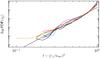 |
Fig. 3 Same as the top bundle of lines in Fig. 2 but
plotted as a function of |

Figure 2 shows the velocity-space density of star particles as a function of 1−ν∥/νesc, and we see that, remarkably, these plots have a reasonably straight section at the highest speeds, just as Leonard & Tremaine (1990) hypothesized. The slopes of these rectilinear sections scatter around k = 3 as we see later.
We also considered the functional form proposed by S07 for the velocity DF; that is,
 . Figure 3 tests this DF with the simulation data. The curvature
implies that this DF does not represent the simulation data as well as the formula proposed
by Leonard & Tremaine (1990).
. Figure 3 tests this DF with the simulation data. The curvature
implies that this DF does not represent the simulation data as well as the formula proposed
by Leonard & Tremaine (1990).
If we fit Eq. (3) to the velocity distributions while fixing k to 3, we recover the escape speeds within 6%. This confirms our choice of the cut-off radius for the gravitational potential, 3R340, that was used during the definition of the escape speeds.
3.1. The velocity threshold
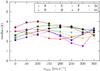 |
Fig. 4 Median values of the likelihood distributions of the power-law index k as a function of the applied threshold velocity νmin. |
We now try to find the best value for the lower threshold velocity νmin. S07 had to use a high threshold value for their radial velocities of 300 km s-1, because the threshold had an additional purpose, namely to select stars from the non-rotating halo component. If one can identify these stars by other means, the velocity threshold can be lowered significantly. This adds more stars to the sample, thereby putting our analysis on a broader basis. If the stellar halo had the shape of an isotropic Plummer (1911) sphere, the threshold could be set to zero, because for this model the S07 version of our approximated velocity distribution function would be exact. However, for other DFs we need to choose a higher value to avoid regions where our approximation breaks down. Again, we use the simulations to select an appropriate value.
We compute the likelihood distribution of k in each simulation using
different velocity thresholds using the likelihood estimator  (7)Figure 4 plots the median values of the likelihood distributions
as a function of the threshold velocity. We see a trend toward increasing
k for νmin ≲ 150 km s-1 and roughly random
behavior above. For low values of νmin, simulation G does not follow the
general trend. This simulation is the only one in the sample that has a dominating bar in
its center (Scannapieco & Athanassoula
2012), which could contain counter-rotating stars. Given this fact, a likely
explanation for its peculiar behavior is that with a low value for the velocity threshold,
bar particles start entering the sample, thereby altering the velocity distribution.
(7)Figure 4 plots the median values of the likelihood distributions
as a function of the threshold velocity. We see a trend toward increasing
k for νmin ≲ 150 km s-1 and roughly random
behavior above. For low values of νmin, simulation G does not follow the
general trend. This simulation is the only one in the sample that has a dominating bar in
its center (Scannapieco & Athanassoula
2012), which could contain counter-rotating stars. Given this fact, a likely
explanation for its peculiar behavior is that with a low value for the velocity threshold,
bar particles start entering the sample, thereby altering the velocity distribution.
Simulation E exhibits a dip around νmin ≃ 300 km s-1. A spatially dispersed stellar stream of significant mass is counter-orbiting the galaxy and is entering the sample at one of the observer positions. This is also clearly visible in Fig. 2 as a bump in one of the velocity distributions between 0.2 and 0.3. Furthermore, this galaxy has a rapidly rotating spheroidal component (Scannapieco et al. 2009).
The galaxy in Simulation C has a satellite galaxy very close by. We exclude all star particles in a radius of 3 kpc around the satellite center from our analysis, but there will still be particles entering our samples that originate in this companion and which do not follow the general velocity DF.
All three cases are unlikely to apply for our Milky Way. Our galaxy hosts a much shorter bar, and up to now no signatures of a massive stellar stream were found in the RAVE data (Seabroke et al. 2008; Williams et al. 2011; Antoja et al. 2012). However, it is very interesting to see how our method performs in these rather extreme cases.
We adopt threshold velocities νmin = 200 km s-1 and 300 km s-1. Both are far enough from the regime where we see systematic evolution in the k values (νmin ≤ 150 km s-1). For the higher value, we can drop the criterion for the particles to be counter-rotating because we can expect the contamination by disk stars to be negligible (S07) and thus partly compensate for the reduced sample size.
3.1.1. An optimal prior for k
From Fig. 4 it seems clear that the different
simulated galaxies do not share exactly the same k, but cover a
considerable range of values. Thus in the analysis of the real data we have to consider
this whole range. We fix the extent of this range by requiring that it delivers optimal
results for all four observer positions in all eight simulated galaxies, so we applied
our analysis to the simulated data by computing the posterior probability distribution
 (8)where
L was defined in Eq. (4), and
(8)where
L was defined in Eq. (4), and  is the
ith rescaled line-of-sight velocity as defined in Eq. (5). We define the median of
p(νesc),
is the
ith rescaled line-of-sight velocity as defined in Eq. (5). We define the median of
p(νesc),  , as the best
estimate. For a comparison of the estimates between different simulations, we consider
the normalized estimate
, as the best
estimate. For a comparison of the estimates between different simulations, we consider
the normalized estimate  with
νesc,true as the true local escape speed in the
simulation. By varying kmin and
kmax, we identify those values that minimize the scatter
in the sample of 32
with
νesc,true as the true local escape speed in the
simulation. By varying kmin and
kmax, we identify those values that minimize the scatter
in the sample of 32  values and at the
same time leave the median of the sample close to unity. We find very similar intervals
for both threshold velocities and adopt the interval
values and at the
same time leave the median of the sample close to unity. We find very similar intervals
for both threshold velocities and adopt the interval
 (9)Reassuringly,
this is very close to the lower part of the interval found by S07 (2.7–4.7) using a
different set of simulations. The scatter of the values is less
than 3.5% (1σ) for both velocity thresholds. This scatter cannot be
completely explained by the statistical uncertainties of the estimates, so there seems
to be an additional uncertainty intrinsic to our analysis technique itself. We try to
quantify this in the next section.
(9)Reassuringly,
this is very close to the lower part of the interval found by S07 (2.7–4.7) using a
different set of simulations. The scatter of the values is less
than 3.5% (1σ) for both velocity thresholds. This scatter cannot be
completely explained by the statistical uncertainties of the estimates, so there seems
to be an additional uncertainty intrinsic to our analysis technique itself. We try to
quantify this in the next section.
3.1.2. Realistic tests
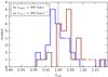 |
Fig. 5 Distribution of |

One important test for our method is whether it still yields correct results if we have imperfect data and a non-isotropic distribution of lines of sights. To simulate typical RAVE measurement errors we attached random Gaussian errors on the parallaxes (distance-1), radial velocities, and the two proper motion values with standard deviations of 30%, 3 km s-1 and 2 mas, respectively. We computed the angular positions of each particle (for a given observer position) and selected only those particles that fell into the approximate survey geometry of the RAVE survey. The latter we define by declination δ < 0° and Galactic latitude | b| > 15°.
Figure 5 shows the resulting distributions of
for the two
velocity thresholds. Again, the width of the distributions cannot be solely explained by
the statistical uncertainties computed from the likelihood distribution, but an
additional uncertainty of ≃4% is required to explain the data in a Gaussian
approximation. The distribution for νmin = 300 km s-1 in addition
exhibits a shift to higher values by ≃3%. Due to the low number statistics the
significance of the shift is unclear (~3σ). As we see in Sect. 5, compared to the statistical uncertainties arising
when we analyze the real data it would presents a minor contribution to the overall
uncertainty and we neglect the shift for this study.
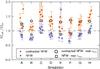 |
Fig. 6 Ratios of the estimated and real virial masses in the eight simulations. For each
simulation, four mass estimates are plotted based on four azimuthal positions of
the Sun in the galaxy. The symbols with error bars represent the estimates based
on the median velocities |

We can go a step further and try to recover the masses of the simulated galaxies using the escape speed estimates. To do this we use the original mass profile of the baryonic components of the galaxies to model our knowledge about the visual parts of the Galaxy and impose an analytic expression for the dark matter halo. As we will do for the real analysis, we try two models: an unaltered and an adiabatically contracted NFW sphere. We adjust the halo parameters, the virial mass M340 and the concentration c, to match both boundary conditions, the circular speed, and the escape speed at the solar radius. Figure 6 plots the ratios of the estimated masses and the real virial masses taken from the simulations directly. The adiabatically contracted halo on average overestimates the virial mass by 25%, while the pure NFW halo systematically understates the mass by about 15%. For both halo models we find examples that obtain a very good match with the real mass (e.g., simulation B for the contracted halo and simulation H for the pure NFW halo). However, the cases where the contracted halo yields better results coincide with those cases where the escape speed was underestimated. The colored symbols in Fig. 6 mark the mass estimates obtained using the exact escape speed computed from the gravitational potential in the simulation directly. This reveals that the mass estimates from the two halo models effectively bracket the real mass as expected. We also recover the masses of the three simulations C, E, and G that show peculiarities in their velocity distributions. Only for simulation E and one azimuthal observer position do we completely fail to recover the mass. In this case there is a prominent stellar stream moving along the line of sight.
4. Data
4.1. The RAVE survey
The major observational data for this study comes from the fourth data release (DR4) of RAVE, a massive spectroscopic stellar survey conducted using the 6dF multi-object spectrograph on the 1.2-m UK Schmidt Telescope at the Siding Springs Observatory (Australia). A general description of the project can be found in the data release papers: Steinmetz et al. (2006), Zwitter et al. (2008), Siebert et al. (2011), and Kordopatis et al. (2013). The spectra are measured in the Ca ii triplet region with a resolution of R = 7000. To provide an unbiased velocity sample, the survey selection function was kept as simple as possible: it is magnitude limited (9 < I < 12) and has a weak color cut of J − Ks > 0.5 for stars near the Galactic disk and the bulge.
In addition to the very precise line-of-sight velocities, νlos, several other stellar properties could be derived from the spectra. Effective temperature Teff, surface gravity log g, and metallicity [M/H] of the stars were estimated several times using different analysis techniques (Zwitter et al. 2008; Siebert et al. 2011; Kordopatis et al. 2011). Breddels et al. (2010), Zwitter et al. (2010), Burnett et al. (2011), and Binney et al. (2013) independently used these estimates to derive spectro-photometric distances for a large fraction of the stars in the survey. Matijevič et al. (2012) performed a morphological classification of the spectra and in this way identified binaries and other peculiar stars. Finally Boeche et al. (2011) developed a pipeline to derive individual chemical abundances from the spectra.
The DR4 contains information for nearly 500 000 spectra of more than 420 000 individual stars. The target catalog was also cross-matched with other databases to be augmented with additional information, such as apparent magnitudes and proper motions. For this study we adopted the distances provided by Binney et al. (2013)3 and the proper motions from the UCAC4 catalog (Zacharias et al. 2013).
4.2. Sample selection
The wealth of information in the RAVE survey presents an ideal foundation for our study. Since S07 the amount of available spectra has grown by a factor of 10, and stellar parameters have become available. The number of high-velocity stars has unfortunately not increased by the same factor, which is most likely because RAVE concentrated more on lower Galactic latitudes where the relative abundance of halo stars – which can have these high velocities – is much lower.
We use only high-quality observations by selecting only stars that fulfill the following criteria:
-
the stars must be classified as “normal” according to the classification by Matijevič et al. (2012),
-
the Tonry-Davis correlation coefficient computed by the RAVE pipeline measuring the quality of the spectral fit (Steinmetz et al. 2006) must be larger than 10,
-
the radial velocity correction due to calibration issues (cf. Steinmetz et al. 2006) must be smaller than 10 km s-1,
-
the signal-to-noise ratio (S/N) must be over 25,
-
the stars must have a distance estimate by Binney et al. (2013),
-
the star must not be associated with a stellar cluster.
The first requirement ensures that the star’s spectrum can be well fitted with a synthetic spectral library and excludes, among other things, spectral binaries. The last criterion removes the giant star (RAVE-ID J101742.6-462715), in particular, from the globular cluster NGC 3201 that would have otherwise entered our high-velocity samples. Stars in gravitationally self-bound structures like globular clusters are clearly not covered by our smooth approximation of the velocity distribution of the stellar halo. We further excluded two stars (RAVE-IDs J175802.0-462351 and J142103.5-374549) because of their peculiar location in the Hertzsprung-Russell diagram4 (cf. Fig. 9, upper panel).
In some cases RAVE observed the same target multiple times. In this case we adopt the measurements with the highest S/N, except for the line-of-sight velocities, νlos, where we use the mean value. The median S/N of the high-velocity stars used in the analysis is 56.
We then convert the precisely measured νlos into the Galactic rest frame using
the following formula:  (10)We define the local
standard of rest, VLSR, to be 220 km s-1, and for
the peculiar motion of the Sun, we adopt the values given by Schönrich et al. (2010): U⊙ = 11.1
km s-1, V⊙ = 12.24 km s-1, and
W⊙ = 7.25 km s-1.
(10)We define the local
standard of rest, VLSR, to be 220 km s-1, and for
the peculiar motion of the Sun, we adopt the values given by Schönrich et al. (2010): U⊙ = 11.1
km s-1, V⊙ = 12.24 km s-1, and
W⊙ = 7.25 km s-1.
As mentioned in Sect. 2 we need to construct a halo sample and we do this in the same way as for the simulation data. We compute the Galactocentric tangential velocities, νφ, of all stars in a Galactocentric cylindrical polar coordinate system using the line-of-sight velocities, proper motions, distances, and the angular coordinates of the stars. For the distance between the Sun and the Galactic center we use the value R0 = 8.28 kpc (Gillessen et al. 2009). We perform a full uncertainty propagation using the Monte-Carlo technique with 2000 resamplings per star to obtain the uncertainties in νφ. As already done for the simulations we discard all stars with positive median estimate of νφ and also those for which the upper end of the 95% confidence interval of νφ reaches above 100 km s-1 to obtain a pure stellar halo sample. This is important because a contamination by stars from the rapidly rotating disk component(s) would invalidate our assumptions made in Sect. 2. Only for this step do we make use of proper motions.
We use the measurements from the UCAC4 catalog (Zacharias et al. 2013) and avoid entries that are flagged as (projected) double star in UCAC4 itself or in one of the additional source catalogs that are used for the proper motion estimate. In such cases we perform the Monte-Carlo analysis with a flat distribution of proper motions between –50 and 50 mas yr-1, both in right ascension, α and declination, δ.
In principle, we could also use a metallicity criterion to select halo stars. There are several reasons why we did not opt for this. First, we want to be able to reproduce our selection in the simulations. Unfortunately, the simulated galaxies are all too metal-poor compared to the Milky Way (Tissera et al. 2012) and are thus not very reliable in this aspect. This is particularly important in the context of the findings by Schuster et al. (2012), who identified correlations between kinematics and metal abundances in the stellar halo that might be related to different origins of the stars (in-situ formation or accretion). However, despite the unrealistic metal abundances, the formation of the stellar halo is modeled realistically in the simulations including all aspects of accretion and in-situ star formation. In the simulated velocity distributions (Fig. 2), we do not detect any characteristic features that would indicate that the duality of the stellar halo as found by Schuster et al. (2012) is relevant for our study. Second, we would have to apply a very conservative metallicity threshold in order to avoid contamination by metal-poor disk stars. Because of this our sample size would not significantly increase using a metallicity criterion instead of a kinematic one.
It is worth mentioning that the star with the highest ν∥ = −448.8 km s-1 in the sample used by S07 (RAVE-ID: J151919.7-191359) did not enter our samples, because it was classified as having problems with the continuum fitting by Matijevič et al. (2012). S07 showed via re-observations that the velocity measurement is reliable, however, the star did not get a distance estimate from Binney et al. (2013). Zwitter et al. (2010) estimate a distance of 9.4 kpc, which owing to its angular position (l,b) = (344.6°,31.4°), would place the star behind and above the Galactic center. The star thus clearly violates the assumption by S07 to deal with a locally confined stellar sample and potentially leads to an overestimate of the escape speed. For the sake of a homogeneous data set, we ignored the alternative distance estimate by Zwitter et al. (2010) and discarded the star.
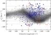 |
Fig. 7 Rescaled radial velocities, |


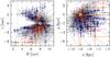 |
Fig. 8 Locations of the stars in our high-velocity sample in the
R-z-plane (left panel) and the
x-y-plane (right panel) as
defined in Fig. 7. Blue and orange symbols
represent RAVE stars and B00 stars, respectively. The error bars show 68% confidence
regions (~1σ). Gray contours show the full RAVE catalog, and the
position of the Sun is marked by a white “⊙”. The dashed lines in both panels mark
locations of constant Galactocentric radius |

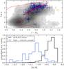 |
Fig. 9 Upper panel: distribution of our high-velocity stars as defined in Fig. 7 in a Hertzsprung-Russell diagram (symbols with blue error bars). For comparison the distribution of all RAVE stars (gray contours) and an isochrone of a stellar population with an age of 10 Gyr and a metallicity of −1 dex (red line) is also shown. The two green symbols represent two stars that were excluded from the samples because of their peculiar locations in this diagram. Lower panel: metallicity distribution of our high-velocity sample (blue histogram). The black histogram shows the metallicity distribution all RAVE stars. |
Figure 7 depicts the velocities
 of all RAVE stars
as a function of Galactic longitude l and the two velocity thresholds
νmin = 200 and 300 km s-1. By selecting for a counter-rotating
(halo) population we automatically select against the general sinusoidal trend of the RAVE
stars in this diagram. Figure 8 illustrates the
spatial distribution of our high-velocity sample. As a result of RAVE avoiding the low
Galactic latitudes, stars with small Galactocentric radii are high above the Galactic
plane. Furthermore, because RAVE is a southern hemisphere survey, the stars in the catalog
are not symmetrically distributed around the Sun. The stars in our high-velocity sample
are mostly giant stars with a metallicity distribution centered at −1.25 dex as can be
seen in Fig. 9.
of all RAVE stars
as a function of Galactic longitude l and the two velocity thresholds
νmin = 200 and 300 km s-1. By selecting for a counter-rotating
(halo) population we automatically select against the general sinusoidal trend of the RAVE
stars in this diagram. Figure 8 illustrates the
spatial distribution of our high-velocity sample. As a result of RAVE avoiding the low
Galactic latitudes, stars with small Galactocentric radii are high above the Galactic
plane. Furthermore, because RAVE is a southern hemisphere survey, the stars in the catalog
are not symmetrically distributed around the Sun. The stars in our high-velocity sample
are mostly giant stars with a metallicity distribution centered at −1.25 dex as can be
seen in Fig. 9.
4.3. Including other literature data
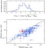 |
Fig. 10 Upper panel: distribution of the differences of the distance modulus estimates, μ, by B00 and Binney et al. (2013), divided by their combined uncertainty for a RAVE-B00 overlap sample of 68 stars. With σBeers = 1.3 mag we find a spread of 1σ in the distribution with the median shifted by 0.6σ ≃ 0.9 mag. The gray curve shows a shifted normal distribution. The two red data points mark two stars which were also entering our high-velocity samples. Lower panel: direct comparison of the two distance estimates with 1 − σ error bars. The solid gray line represents equality, while the dashed-dotted line marks equality after reducing the B00 distances by a factor of 1.5. |
To increase our sample sizes we have also considered other publicly available and kinematically unbiased data sets. We used the sample of metal-poor dwarf stars collected by Beers et al. (2000, B00 hereafter). The authors also provided the full 6D phase space information including photometric parallaxes. We updated the proper motions by cross-matching with the UCAC4 catalog (Zacharias et al. 2013). We found new values for 2011 stars using the closest counterparts within a search radius of 5 arcsec. For ten stars we found two sources in the UCAC4 catalog closer than 5 arcsec, so discarded these stars. There were a further five cases where two stars in the B00 catalog have the same closest neighbor in the UCAC4 catalog. All these ten stars were discarded as well. Finally, we kept only those stars with uncertainties in the line-of-sight velocity measurement below 15 km s-1.
There is a small overlap of 123 stars with RAVE, 68 of which have a parallax estimate, ϖ, by Binney et al. (2013) with σ(ϖ) < ϖ. By chance two of these stars entered our high-velocity samples. This, on first glance, very unlikely event is not so surprising if we consider our selection for halo stars, the strong bias towards metal-poor halo stars of the B00 catalog, and the significant completeness of the RAVE survey >50% in the brighter magnitude bins (Kordopatis et al. 2013).
To compare the two distance estimates, we convert all distances, d, into distance moduli, μ = 5log (d/10 pc), because both estimates are based on photometry, so the error distribution should be approximately5 symmetric in this quantity. We find that σBeers should be about 1.3 mag for the weighted differences (Fig. 10, upper panel) to have a standard deviation of unity. B00 quote an uncertainty of 20% on their photometric parallax estimates, while our estimate corresponds to roughly 60%. We adopt our more conservative value and emphasize that this uncertainty is only used during the selection of counter-rotating halo stars.
We further find a systematic shift by a factor fdist = 1.5
(δμ = 0.9 mag) between the two distance estimates, in the sense that
the B00 distances are greater. Since more information was taken into account to derive the
RAVE distances we consider them more reliable. To have consistent distances, we decrease
all B00 distances by  and use these calibrated values in our further analysis.
The data set with the currently most accurately estimated 6D phase space coordinates is the Geneva-Copenhagen survey (Nordström et al. 2004) providing Hipparcos distances and proper motions, as well as precise radial velocity measurements. However, this survey is confined to a very small volume around the Sun and is therefore even more strongly dominated by disk stars than the RAVE survey. We find only two counter-rotating stars in this sample with | ν∥| > 200 km s-1, as well as two (co-rotating) stars with | ν∥| > 300 km s-1. For the sake of homogeneity in our sample we neglect these measurements.
5. Results
5.1. Comparison to Smith et al. (2007)
As a first check we did an exact repetition of the analysis applied by S07 to see whether
we get a consistent result. This is interesting because strong deviations could point to
possible biases in the data due to, say, the slightly increased survey footprint of the
sky. RAVE contains 76 stars fulfilling the criteria, which is an increase by a factor 5 (3
if we take the 19 stars from the B006 catalog into
account). The median values of the distributions are effectively the same (537
km s-1 instead of 544 km s-1), and the uncertainties resulting
from the 90% confidence interval ([504,574]) are reduced by a factor 0.6 (0.7) for the
upper (lower) margin. If we assume that the precision is proportional to the square root
of the sample size, we expect a decrease in the uncertainties of a factor
 .
.
With the distance estimates available now, we know that this analysis rests on the
incorrect assumption that we are dealing with a local sample. If we apply a distance cut
dmax = 2.5 kpc onto the data we obtain a sample of 15 RAVE
stars and 16 stars from the B00 catalog, and we compute a median estimate of
 km s-1. A lower value is expected because the distance criteria mainly
removes stars from the inner Galaxy where stars generally have higher velocities. The
reason for this is that RAVE is a southern hemisphere survey and therefore observes mostly
the inner Galaxy.
km s-1. A lower value is expected because the distance criteria mainly
removes stars from the inner Galaxy where stars generally have higher velocities. The
reason for this is that RAVE is a southern hemisphere survey and therefore observes mostly
the inner Galaxy.
5.2. The local escape speed
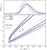 |
Fig. 11 Likelihood distributions of parameter pairs νesc,k (lower panel). The positions of the maximum likelihood pairs are marked with the symbols “×” for the V200 samples and “+” for the V300 samples. Contour lines mark the locations where the likelihood dropped to 10% and 1% of the maximum value. The upper panel shows the likelihood distributions marginalized over the most likely k-interval [2.3, 3.7]. |
As described as option (2) in Sect. 2.1, we can
estimate for all stars in the catalogs what their radial velocity would be if they were
situated at the position of the Sun. We then create two samples using the new velocities.
For the first sample we select all stars with rescaled velocities
 km s-1. S07 shows that such a high velocity threshold predominantly yields
halo stars. The resulting sample contains 53 stars (34 RAVE stars), and we refer to it as
V300. The second sample has a lower velocity threshold of 200 km s-1, but stars
are preselected, in analogy to the simulation analysis, considering only stars classified
as “halo” (Sect. 4.2). This sample we call V200, and
it contains 86 stars (69 RAVE stars). Most of the stars are located closer to the Galactic
center than the Sun and thus the correction mostly leads to decreased velocity values. In
both samples, about 7% of the stars have repeat observations. The maximum difference
between two velocity measurements is 2.5 km s-1.
km s-1. S07 shows that such a high velocity threshold predominantly yields
halo stars. The resulting sample contains 53 stars (34 RAVE stars), and we refer to it as
V300. The second sample has a lower velocity threshold of 200 km s-1, but stars
are preselected, in analogy to the simulation analysis, considering only stars classified
as “halo” (Sect. 4.2). This sample we call V200, and
it contains 86 stars (69 RAVE stars). Most of the stars are located closer to the Galactic
center than the Sun and thus the correction mostly leads to decreased velocity values. In
both samples, about 7% of the stars have repeat observations. The maximum difference
between two velocity measurements is 2.5 km s-1.
The resulting likelihood distribution in the (νesc,k) parameter plane is shown in the lower panel of Fig. 11. The maximum likelihood pairs for the different samples agree very well, except for the pair constructed from RAVE-only V300 sample, which is located near νesc ≃ 410 km s-1 and k ≃ 0. In all cases a clear degeneracy between k and the escape speed is visible. This was already seen by S07 and reflects that a similarly curved form of the velocity DF over the range of radial velocities available by different parameter pairs.
Median and 90% confidence limits from different analysis strategies.
We go further and compute the posterior probability DF for νesc, p(νesc) using Eq. (8), which effectively means that we marginalize over the optimized k-interval derived in Sect. 3.1.1. For the medians of these distributions, we obtain higher values than the maximum likelihood value for all samples. This behavior is consistent with our findings in Sect. 2.2 where we showed that the maximum likelihood analysis tends to yield pairs with too low values for k and νesc. These median values can be found in Table 3 (“Localized”).
5.3. Binning in Galactocentric distance
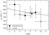 |
Fig. 12 Escape speed estimates and 90% confidence intervals in Galactocentric radial bins. The solid black line shows our best-fitting model. Only the filled black data points were used in the fitting process. The red data point illustrates the result of our “localized” approach. |
For halo stars with original | ν∥| ≥ 200 km s-1, we are able to fill several bins in Galactocentric distance r and thereby perform a spatially resolved analysis as described as option (1) in Sect. 2.1. We chose six overlapping bins with a radial width of 2 kpc between 4 and 11 kpc. This bin width is larger than the uncertainties of the projected radius estimates for almost all our sample stars (cf. Fig. 8). The number of stars in the bins are 11, 28, 44, 52, 35, and 8. The resulting median values (again after marginalizing over the optimal k-interval) of the posterior PDF and the 90% confidence intervals are plotted in Fig. 12. The values near the Sun are in very good agreement with the results of the previous section. We find a rather flat escape-speed profile except for the outmost bins, which contain very few stars, though, and thus have large confidence intervals.
6. Discussion
6.1. Influence of the input parameters
The 90% confidence intervals provided by our analysis technique only reflect the statistical uncertainties resulting from the finite number of stars in our samples. In this section we consider systematic uncertainties. In Sect. 3.1.2 we already showed that our adopted interval for the power-law index k introduces a systematic scatter of about 4%.
A further source of uncertainties comes from the motion of the Sun relative to the Galactic center. While the radial and vertical motion of the Sun is known to very high precision, several authors have come to different conclusions about the tangential motion, V⊙ (e.g., Reid & Brunthaler 2004; Bovy et al. 2012; Schönrich 2012). In this study we used the standard value for VLSR = 220 km s-1 and the V⊙ = 12.24 km s-1 from Schönrich et al. (2010). We repeated the whole analysis using VLSR = 240 km s-1 and compared the resulting escape speeds with the values of our standard analysis (cf. the lower part of Table 3). The magnitudes of the deviations are statistically not significant, but we find systematically lower estimates of the local escape speed for the higher value of VLSR. The shift is close to 20 km s-1 and thus comparable to the difference ΔVLSR. This can be understood if we consider that most stars in the RAVE survey and also in our samples are observed at negative Galactic longitudes and thus against the direction of Galactic rotation (see Fig. 7). In this case correcting the measured heliocentric line-of-sight velocities with a higher solar tangential motion leads to lower ν∥ which eventually reflects into the escape speed estimate. This systematic dependency is induced by the half-sky nature of the RAVE survey, while this effect might cancel out for an all-sky survey. In contrast, the exact value of R0 does not influence our results, as long as it is kept within the range of proposed values around 8 kpc.
The quantity with the largest uncertainties used in this study is the heliocentric distance of the stars. In Sect. 4.3 we found a systematic difference between the distances derived for the RAVE stars and for the stars in the B00 catalog. Such systematic shifts can arise for various reasons: e.g., different sets of theoretical isochrones, systematic errors in the stellar parameter estimates, or different extinction laws. Again we repeated our analysis, this time with all distances increased by a factor 1.5, practically moving to the original distance scale of B00. Again we find a systematic shift to lower local escape speeds of the same order as for the alternative value of VLSR.
We finally also tested the influence of the Galaxy model we use to rescale the stellar velocities according to their spatial position. We changed the disk mass to 6.5 × 10¹⁰ M⊙ and decreased the disk scale radius to 2.5 kpc, in this way preserving the local surface density of the standard model. The resulting differences in the corrected velocities are below 1%, and no measurable difference in the escape speed estimates was found, illustrating the robustness of our methods to reasonable changes in the Galaxy parameters.
6.2. A critical view of the input assumptions
Our analysis stands and falls with the reliability of our approximation of the velocity DF given in Eq. (1). The conceptual underpinning of this approximation is very weak for four reasons:
-
In many analytic equilibrium models of stellar systems at any spatial point, there is a non-zero probability density of finding a star right up to the escape speed νesc at that point, and zero probability at higher speeds. For example, the Jaffe (1983) and Hernquist (1990) models have this property but King-Michie models (King 1966) do not: in these models the probability density falls to zero at a speed that is less than the escape speed. There is thus an important counterexample to the proposition that n(ν) first vanishes at ν= νesc.
-
All theories of galaxy formation, including the standard ΛCDM paradigm, predict that the velocity distribution becomes radially biased at high speed, so in the context of an equilibrium model, there must be significant dependence of the DF on the total angular momentum J in addition to E.
-
As Spitzer & Thuan (1972) pointed out, in any stellar system, as E → 0, the periods of orbits diverge. Consequently the marginally-bound part of phase space cannot be expected to be phase mixed. Specifically, stars that are accelerated to speeds just short of νesc by fluctuations in Φ in the inner system take arbitrarily long times to travel to apocenter and return to radii where we may hope to study them. As a result different mechanisms populate the outgoing and incoming parts of phase space at speeds ν~ νesc: while parts are populated by cosmic accretion (Abadi et al. 2009; Teyssier et al. 2009; Piffl et al. 2011), the outgoing part in addition is populated by slingshot processes (e.g., Hills 1988; Brown et al. 2005) and violent relaxation in the inner galaxy. It follows that we cannot expect the distribution of stars in this portion of phase space to conform to Jeans theorem, even approximately. Equation (1) is founded not just on Jeans theorem but on a very special form of it.
-
Counts of stars in the Sloan Digital Sky Survey (SDSS) have most beautifully demonstrated that the spatial distribution of high-energy stars is very non-smooth. The origin of these fluctuations in stellar density is widely acknowledged to be the impact of cosmic accretion, which ensures that at high energies the DF does not satisfy Jeans theorem.
From this discussion it should be clear that to obtain a credible relationship between the density of fast stars and νesc, we must engage with the processes that place stars in the marginally bound part of phase space. Fortunately, sophisticated simulations of galaxy formation in a cosmological context do just that. Figure 2 illustrates that Eq. (1) catches the general shape of the velocity DF very well. That we find a relatively small interval for the power-law index k that fits all simulated galaxies with their variety of morphologies argues for the appropriateness of the functional form by Leonard & Tremaine (1990).
The question remains whether the applied simulation technique influences the range of k-values we find, since all eight galaxy models were produced with the same simulation code. In particular, the numerical recipes for so-called sub-grid physics like star formation and stellar energy feedback can have a significant impact on the simulation result as recently demonstrated in the Aquila code comparison project (Scannapieco et al. 2012). However, the main differences were found in the formation of galaxy disks, while in this study we explicitly focus on the stellar halo that was built up from infalling satellite galaxies. Differing implementations of subgrid physics might change the amount of stellar and gas mass being brought in by small galaxies, but it appears unlikely that the phase-space structure of the Galactic halo will change significantly. This view is confirmed by the very similar k-interval found by S07 using simulations with a completely different implementation of subgrid physics.
6.3. Estimating the mass of the Milky Way
We now attempt to derive the total mass of the Galaxy using our escape speed estimates.
Doing this we exploit the fact that the escape speed is a measure of the local depth of
the potential well  . A critical
point in our methodology is the question whether the velocity distribution reaches up to
νesc or whether it is truncated at some lower value. S07 used their
simulations to show that the level of truncation in the stellar component cannot be more
than 10%. However, to test this they first had to define the local escape speed by fixing
a limiting radius beyond which a star is considered unbound. The authors state explicitly
that the choice of this radius as 3Rvir is rather arbitrary.
More stringent would be to state that the velocity distribution in the simulations point
to a limiting radius of ~3Rvir beyond which stars do not fall
back onto the galaxy or fall back only with significantly altered orbital energies, e.g.,
as part of an infalling satellite galaxy.
. A critical
point in our methodology is the question whether the velocity distribution reaches up to
νesc or whether it is truncated at some lower value. S07 used their
simulations to show that the level of truncation in the stellar component cannot be more
than 10%. However, to test this they first had to define the local escape speed by fixing
a limiting radius beyond which a star is considered unbound. The authors state explicitly
that the choice of this radius as 3Rvir is rather arbitrary.
More stringent would be to state that the velocity distribution in the simulations point
to a limiting radius of ~3Rvir beyond which stars do not fall
back onto the galaxy or fall back only with significantly altered orbital energies, e.g.,
as part of an infalling satellite galaxy.
It is not a conceptual problem to define the escape speed as the high end of the velocity
distribution in disregard of the potential profile outside the corresponding limiting
radius. Then it is important, however, to use the same limiting radius while deriving the
total mass of the system using an analytic profile. This means we have to redefine the
escape speed to  (11)where
Rmax = 3R340 seems to be an
appropriate value (cf. Sect. 3).
(11)where
Rmax = 3R340 seems to be an
appropriate value (cf. Sect. 3).
This leads to somewhat higher mass estimates. For example, S07 found an escape speed of 544 km s-1 and derived a halo mass of 0.85 × 10¹² M⊙ for an NFW profile, practically using Rmax = ∞. If one consistently applies Rmax = 3Rvir, the resulting halo mass is 1.05 × 10¹² M⊙, an increase by more than 20%. This is the reason our mass estimates are higher than those by S07 even though we find a similar escape speed. These values represent the masses of the dark matter halo alone, while in the remainder of this study we mean the total mass of the Galaxy when we refer to the virial mass M340. Keeping this in mind it is then straightforward to compute the virial mass corresponding to a certain local escape speed. As already mentioned, we use the simple mass model presented in Sect. 2.
In the case of the escape speed profile obtained via the binned data, the procedure
becomes slightly more elaborate. We have to compute the escape speeds at the centers of
the radial bins Ri and then take the
likelihood from the probability distributions
PDFRi(νesc) in
each bin. The product of all these likelihoods7 is
the general likelihood assigned to the mass of the model, i.e.,
 (12)The results of these mass
estimates are presented in Table 3. As already seen
in Fig. 6 for the simulations the adiabatically
contracted halo model always yields higher results than the unaltered halo.
(12)The results of these mass
estimates are presented in Table 3. As already seen
in Fig. 6 for the simulations the adiabatically
contracted halo model always yields higher results than the unaltered halo.
6.4. Fitting the halo concentration parameter
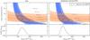 |
Fig. 13 Likelihood distribution resulting from our simple Galaxy model when we leave the halo concentration c (and therefore also VLSR) as a free parameter (blue area) for an NFW profile as halo model (left panel) and an adiabatically contracted NFW profile (right panel). The red contours arise when we add the constraints on c from cosmological simulations: the relation of the mean c for a given halo mass found by Macciò et al. (2008) is represented by the thick dashed orange line. The orange area illustrates the spread around the mean c values found in the simulations. The different shades in the blue and orange colored areas mark locations where the probability dropped to 10%, 1% of the maximum value as do the black contour lines for the combined likelihood distribution. Dotted gray lines connect locations with constant circular speed at the solar radius. |
Up to now we have assumed a fixed value for the local standard of rest, VLSR = 220 km s-1, to reduce the number of free parameters in our Galaxy model to one. Recently, several authors have found higher values for VLSR of up to 240 km s-1 (e.g., Bovy et al. 2012; Schönrich 2012). If we change the parametrization in the model and use the halo concentration c as a free parameter, we can compute the likelihood distribution in the (M340,c)-plane in the same way as described in the previous section. Figure 13 plots the resulting likelihood contours for an NFW halo profile (left panel) and the adiabatically contracted NFW profile (right panel).
Navarro et al. (1997) showed that the concentration parameter is strongly related to the mass and the formation time of a dark matter halo (see also Neto et al. 2007; Macciò et al. 2008; Ludlow et al. 2012). With this information we can constrain the range of likely combinations (M340,c) further. We use the relation for the mean concentration as a function of halo mass proposed by Macciò et al. (2008). For this we converted their relation for c200 to c340 to be consistent with our definition of the virial radius. There is significant scatter around this relation reflecting the variety of formation histories of the halos. This scatter is reasonably well fitted by a log-normal distribution with σlog c = 0.11 (e.g. Macciò et al. 2008; Neto et al. 2007). If we apply this as a prior to our likelihood estimation we obtain the black solid contours plotted in Fig. 13. In the adiabatically contracted case the concentration parameters we are quoting are the initial concentrations before the contraction. Only these are comparable to results obtained from dark matter-only simulations.
The maximum likelihood pair of values (marked by a black “+” in the figure) for the normal NFW halo is M340 = 1.37 × 10¹² M⊙ and c = 5, which implies a circular speed of 196 km s-1 at the solar radius. The adiabatically contracted NFW profile yields the same c but a somewhat lower mass of 1.22 × 10¹² M⊙. Here the resulting circular speed is only 236 km s-1.
If we marginalize the likelihood distribution along the c-axis we obtain
the one-dimensional posterior PDF for the virial mass. The median and the 90% confidence
interval we find to be  for
the unaltered halo profile. For the adiabatically contracted NFW profile we find
for
the unaltered halo profile. For the adiabatically contracted NFW profile we find
 in
both cases almost identical to the maximum likelihood value. It is worth noting that in
this approach, the adiabatically contracted halo model yields the lower mass estimate,
while the opposite was the case when we fixed the local standard of rest as done in the
previous section.
in
both cases almost identical to the maximum likelihood value. It is worth noting that in
this approach, the adiabatically contracted halo model yields the lower mass estimate,
while the opposite was the case when we fixed the local standard of rest as done in the
previous section.
There are several definitions of the virial radius used in the literature. In this study
we used the radius which encompasses a mean density of 340 times the critical density for
closure in the universe. If one adopts an overdensity of 200, the resulting masses
M200 increase to  M⊙
and
M⊙
and  M⊙
for the pure and the adiabatically contracted halo profiles, respectively. For an
overdensity of 340 Ω0 ~ 100 (Ω0 = 0.3 being the cosmic mean matter
density), as used, say, by Smith et al. (2007) or
Xue et al. (2008), the values even increase to
M⊙
for the pure and the adiabatically contracted halo profiles, respectively. For an
overdensity of 340 Ω0 ~ 100 (Ω0 = 0.3 being the cosmic mean matter
density), as used, say, by Smith et al. (2007) or
Xue et al. (2008), the values even increase to
 M⊙
and
M⊙
and  M⊙.
The corresponding virial radii are
M⊙.
The corresponding virial radii are  for
both halo profiles (R200 = 225 ± 20 kpc).
for
both halo profiles (R200 = 225 ± 20 kpc).
6.5. Relation to other mass estimates
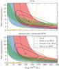 |
Fig. 14 Additional constraints on the parameter pairs (M340,c) coming from studies from the literature. The black contours are the same as in Fig. 13. Gnedin et al. (2010) measured the mass interior to 80 kpc from the GC, Xue et al. (2008) within 60 kpc and Kafle et al. (2012) inside 25 kpc. The yellow solid and dotted line separate models for which the satellite galaxy Leo I is on a bound orbit (below the lines) from those where it is unbound. |
As further constraints we can include literature estimates of total masses inside various Galactocentric radii by Xue et al. (2008), Gnedin et al. (2010), and Kafle et al. (2012). Gnedin et al. (2010) obtained an estimate of a mass of 6.9 × 10¹¹ M⊙ ± 20% within 80 kpc via Jeans modeling using radial velocity measurements of halo stars between 25 and 80 kpc from the Hypervelocity Star Survey. Xue et al. (2008) find a mass within 60 kpc of 4.0 ± 0.7 × 10¹¹ M⊙ by reconstructing the circular velocity curve using a radial velocities of halo BHB stars from the SDSS combined with cosmological simulations. Kafle et al. (2012) measured a Galactic mass of 2.1 × 10¹¹ M⊙ within 25 kpc of the Galactic center using a similar data set to Xue et al. (2008), but restricting themselves to stars closer than 25 kpc for which proper motion measurements were available. In this way Kafle et al. (2012) did not have to rely on additional simulation data. We use a 68% confidence interval of [1.8,2.3] × 1012 M⊙ for this last estimate (green shaded area; P. Kafle, priv. comm.). Models fulfilling these constraints are marked in Fig. 14 with colored shaded areas. In the case of the unaltered NFW halo we find excellent agreement with Gnedin et al. (2010) and Kafle et al. (2012), while for the adiabatically contracted model the combination of these estimates favor higher virial masses. The estimate by Xue et al. (2008) is only barely consistent with our results on a 1σ-level for both halo models.
Tests with a different model for the Galactic disk (Md = 6.5 × 10¹⁰ M⊙, Rd = 2.5 kpc, similar to the one used by Kafle et al. 2012 and Sofue et al. 2009) resulted in decreased mass estimates (10%), well within the uncertainties. This model changes the values for the circular speed (223 km s-1 and 264 km s-1 for the unaltered and the contracted cases, respectively) but not the consistency with the mass estimates by Kafle et al. (2012), Gnedin et al. (2010), or Xue et al. (2008).
Another important constraint for the Galactic halo is the space motion of the satellite
galaxy Leo I. Boylan-Kolchin et al. (2013) show
that in the ΛCDM paradigm, it is extremely unlikely that a galaxy like the Milky Way has
an unbound close-by satellite galaxy. If we take the recent estimates for the
Galactocentric distance of 261 ± 13 kpc and the absolute space velocity of
 km s-1 (Sohn et al. 2013), we can
identify those combinations of M340 and c
that leave Leo I on a bound orbit. The line separating models in which Leo I is bound from
those where it is not bound is also plotted in Fig. 14. All models below this line are consistent with a bound orbit of Leo I. The
uncertainties are also shown in the figure in the sense that they mark the ridge lines for
the extreme cases that Leo I is slower and closer by 1σ and that it is
farther and faster by 1σ. In the case of the unaltered halo profile, our
mass estimate is consistent with Leo I being on a bound orbit, while in the contracted
case, the mass of the Galaxy would be too low.
km s-1 (Sohn et al. 2013), we can
identify those combinations of M340 and c
that leave Leo I on a bound orbit. The line separating models in which Leo I is bound from
those where it is not bound is also plotted in Fig. 14. All models below this line are consistent with a bound orbit of Leo I. The
uncertainties are also shown in the figure in the sense that they mark the ridge lines for
the extreme cases that Leo I is slower and closer by 1σ and that it is
farther and faster by 1σ. In the case of the unaltered halo profile, our
mass estimate is consistent with Leo I being on a bound orbit, while in the contracted
case, the mass of the Galaxy would be too low.
Finally, Przybilla et al. (2010) found a star,
J1539+0239, with a velocity of  km s-1 at a Galactocentric distance of ~8 kpc moving inwards to the Galaxy.
The authors argue that this star should therefore be bound to the Milky Way (see also
Irrgang et al. 2013). The star is not in the
solar vicinity since its heliocentric distance was measured as 12 ± 2.3 kpc, but its
Galactocentric distance is comparable to R0. We can therefore
directly compare our results. Owing to the large uncertainties in the velocity estimate,
it is not surprising that our most likely value for νesc is consistent with
J1539+0239 being on a bound orbit. However, if their median velocity is correct, this star
is clearly unbound in our model of the Galaxy and must have obtained its high speed via
some other mechanism or be of extragalactic origin.
km s-1 at a Galactocentric distance of ~8 kpc moving inwards to the Galaxy.
The authors argue that this star should therefore be bound to the Milky Way (see also
Irrgang et al. 2013). The star is not in the
solar vicinity since its heliocentric distance was measured as 12 ± 2.3 kpc, but its
Galactocentric distance is comparable to R0. We can therefore
directly compare our results. Owing to the large uncertainties in the velocity estimate,
it is not surprising that our most likely value for νesc is consistent with
J1539+0239 being on a bound orbit. However, if their median velocity is correct, this star
is clearly unbound in our model of the Galaxy and must have obtained its high speed via
some other mechanism or be of extragalactic origin.
6.6. Dark matter halo profile
The two halo models, unaltered and adiabatically contracted NFW halos, are rather extreme cases, and the true shape of the Galactic halo is most likely intermediate to these options (Abadi et al. 2010). When we fixed the circular speed at the Sun’s position (as done for the estimates shown in Table 3), the resulting halo masses strongly depended on the shape of the profile. However, when we loosened this constraint using a prior on the halo concentration c (as in Sect. 6.4), our mass estimates became fairly robust to changes of the halo model. In this approach the tension between the constraints coming from the circular speed at the solar radius, and the mass estimates at larger distances are likely to be resolved by an intermediate halo model as proposed by Abadi et al. (2010).
6.7. Future prospects
The ESO cornerstone mission Gaia (Prusti 2012) will soon revolutionize the field of Galactic astronomy. It will deliver the full 6D phase space information for more 100 million stars in the extended solar neighborhood. With these data we will no longer be restricted to the use of radial velocities alone because tangential velocities with similar or even smaller uncertainties will be available. Repeating our analysis with Gaia observations will therefore deliver much more precise results.
On the other hand, we expect that the full complexity of the Galaxy will appear in these data as well. The comparatively sparse RAVE data allowed neglecting many of the details of the Galactic structure, in particular the clumpy nature of the stellar halo. This might no longer be possible with the Gaia data, or in other words, the precision of the estimate might no longer be limited by the data, but by the assumptions in the analysis method itself. It is thus possible that the gain is smaller than one might naively expect if the analysis is repeated in the exact same manner. More robust knowledge about the structure of the inner galaxy obtained, for example, via the analysis of cold tidal streams (Koposov et al. 2010; Sanders & Binney 2013) might make it possible to refine these assumptions.
7. Conclusions
In the present study we analyzed the latest data release of the RAVE survey (fourth data release, Kordopatis et al. 2013), together with additional literature data, to estimate the Galactic escape speed (νesc) at various Galactocentric radial bins and, through this, the virial mass of our Galaxy. For it we defined the escape speed as the minimum speed required to reach 3R340. To break a degeneracy between our fitting parameters, we had to calibrate our method on a set of cosmological simulations of disk galaxy formation. The 90% confidence interval for our best estimate of the local escape speed is 492 < νesc < 587 km s-1, with a median value of 533 km s-1.
With our new νesc value, we can estimate the virial mass of the Galaxy (baryons and dark matter) by assuming a simple mass model of the baryonic content of the Galaxy and a spherical (adiabatically contracted) NFW halo profile and by using the local standard of rest, VLSR, as an additional constraint. The resulting values can be found in Table 3.
The value of VLSR is still under debate. If we loosen our
constraint on VLSR and use a prior on the halo concentration
parameter, c, coming from large cosmological simulations we find a most
likely value for the virial mass  M⊙
for the pure NFW profile and
M⊙
for the pure NFW profile and  M⊙
for an adiabatically contracted halo profile.
M⊙
for an adiabatically contracted halo profile.
In Sect. 6.5 we compared our results to other mass estimates. We found good agreement with estimates based on distant halo stars as well as the space motion of the satellite galaxy Leo I.
Note, that the definition of the virial radius differs for different authors. For our final mass estimate in Sect. 6.4 we also provide the corresponding masses for other definitions.
We actually used the parallax estimates, as these are more robust according to Binney et al. (2013).
Binney et al. (2013) actually showed that the RAVE parallax uncertainty distribution is close to normal. However, since both the RAVE and the B00 distances are based on the apparent magnitudes of the stars, comparing the distance moduli seems to be the better choice, even though the uncertainties are not driven by the uncertainties in the photometry.
Acknowledgments
T.P. and M.S. acknowledge support by the German Research Foundation under grant DFG-STE-710/4-3. Funding for RAVE has been provided by the Australian Astronomical Observatory, the Leibniz-Institut für Astrophysik Potsdam (AIP), the Australian National University, the Australian Research Council, the French National Research Agency, the German Research Foundation (SPP 1177 and SFB 881), the European Research Council (ERC-StG 240271 Galactica), the Istituto Nazionale di Astrofisica at Padova, The Johns Hopkins University, the National Science Foundation of the USA (AST-0908326), the W. M. Keck foundation, the Macquarie University, the Netherlands Research School for Astronomy, the Natural Sciences and Engineering Research Council of Canada, the Slovenian Research Agency, the Swiss National Science Foundation, the Science & Technology Facilities Council of the UK, Opticon, Strasbourg Observatory, and the Universities of Groningen, Heidelberg, and Sydney. The RAVE web site is at http://www.rave-survey.org. This research made use of the cross-match service provided by the CDS, Strasbourg. This research made use of the SIMBAD database, operated at CDS, Strasbourg, France. This research has made use of the VizieR catalogue access tool, CDS, Strasbourg, France.
References
- Abadi, M. G., Navarro, J. F., Steinmetz, M., & Eke, V. R. 2003, ApJ, 597, 21 [NASA ADS] [CrossRef] [MathSciNet] [Google Scholar]
- Abadi, M. G., Navarro, J. F., & Steinmetz, M. 2009, ApJ, 691, L63 [NASA ADS] [CrossRef] [Google Scholar]
- Abadi, M. G., Navarro, J. F., Fardal, M., Babul, A., & Steinmetz, M. 2010, MNRAS, 407, 435 [NASA ADS] [CrossRef] [Google Scholar]
- Alexander, J. B. 1982, MNRAS, 201, 579 [NASA ADS] [Google Scholar]
- Antoja, T., Helmi, A., Bienaymé, O., et al. 2012, MNRAS, 426, L1 [NASA ADS] [CrossRef] [Google Scholar]
- Battaglia, G., Helmi, A., Morrison, H., et al. 2005, MNRAS, 364, 433 [NASA ADS] [CrossRef] [Google Scholar]
- Battaglia, G., Helmi, A., Morrison, H., et al. 2006, MNRAS, 370, 1055 [NASA ADS] [CrossRef] [Google Scholar]
- Beers, T. C., Chiba, M., Yoshii, Y., et al. 2000, AJ, 119, 2866 (B00) [NASA ADS] [CrossRef] [Google Scholar]
- Binney, J., Burnett, B., Kordopatis, G., et al. 2013, MNRAS, 437, 351 [Google Scholar]
- Boeche, C., Siebert, A., Williams, M., et al. 2011, AJ, 142, 193 [NASA ADS] [CrossRef] [Google Scholar]
- Bovy, J., Allen de Prieto, C., Beers, T. C., et al. 2012, ApJ, 759, 131 [NASA ADS] [CrossRef] [Google Scholar]
- Boylan-Kolchin, M., Besla, G., & Hernquist, L. 2011, MNRAS, 414, 1560 [NASA ADS] [CrossRef] [Google Scholar]
- Boylan-Kolchin, M., Bullock, J. S., Sohn, S. T., Besla, G., & van der Marel, R. P. 2013, ApJ, 768, 140 [NASA ADS] [CrossRef] [Google Scholar]
- Breddels, M. A., Smith, M. C., Helmi, A., et al. 2010, A&A, 511, A90 [NASA ADS] [CrossRef] [EDP Sciences] [Google Scholar]
- Brown, W. R., Geller, M. J., Kenyon, S. J., & Kurtz, M. J. 2005, ApJ, 622, L33 [NASA ADS] [CrossRef] [Google Scholar]
- Burnett, B., Binney, J., Sharma, S., et al. 2011, A&A, 532, A113 [NASA ADS] [CrossRef] [EDP Sciences] [Google Scholar]
- Busha, M. T., Marshall, P. J., Wechsler, R. H., Klypin, A., & Primack, J. 2011, ApJ, 743, 40 [NASA ADS] [CrossRef] [Google Scholar]
- Deason, A. J., Belokurov, V., Evans, N. W., et al. 2012, MNRAS, 425, 2840 [NASA ADS] [CrossRef] [Google Scholar]
- Fich, M., & Tremaine, S. 1991, ARA&A, 29, 409 [Google Scholar]
- Gillessen, S., Eisenhauer, F., Fritz, T. K., et al. 2009, ApJ, 707, L114 [NASA ADS] [CrossRef] [Google Scholar]
- Gnedin, O. Y., Brown, W. R., Geller, M. J., & Kenyon, S. J. 2010, ApJ, 720, L108 [NASA ADS] [CrossRef] [Google Scholar]
- Hernquist, L. 1990, ApJ, 356, 359 [NASA ADS] [CrossRef] [Google Scholar]
- Hills, J. G. 1988, Nature, 331, 687 [Google Scholar]
- Irrgang, A., Wilcox, B., Tucker, E., & Schiefelbein, L. 2013, A&A, 549, A137 [NASA ADS] [CrossRef] [EDP Sciences] [Google Scholar]
- Jaffe, W. 1983, MNRAS, 202, 995 [NASA ADS] [Google Scholar]
- Kafle, P. R., Sharma, S., Lewis, G. F., & Bland-Hawthorn, J. 2012, ApJ, 761, 98 [NASA ADS] [CrossRef] [Google Scholar]
- Kallivayalil, N., van der Marel, R. P., Besla, G., Anderson, J., & Alcock, C. 2013, ApJ, 764, 161 [NASA ADS] [CrossRef] [Google Scholar]
- King, I. R. 1966, AJ, 71, 64 [Google Scholar]
- Kochanek, C. S. 1996, ApJ, 457, 228 [NASA ADS] [CrossRef] [Google Scholar]
- Koposov, S. E., Rix, H.-W., & Hogg, D. W. 2010, ApJ, 712, 260 [NASA ADS] [CrossRef] [Google Scholar]
- Kordopatis, G., Recio-Blanco, A., de Laverny, P., et al. 2011, A&A, 535, A106 [NASA ADS] [CrossRef] [EDP Sciences] [Google Scholar]
- Kordopatis, G., Gilmore, G., Steinmetz, M., et al. 2013, AJ, 146, 134 [NASA ADS] [CrossRef] [Google Scholar]
- Leonard, P. J. T., & Tremaine, S. 1990, ApJ, 353, 486 [NASA ADS] [CrossRef] [Google Scholar]
- Li, Y.-S., & White, S. D. M. 2008, MNRAS, 384, 1459 [NASA ADS] [CrossRef] [Google Scholar]
- Ludlow, A. D., Navarro, J. F., Li, M., et al. 2012, MNRAS, 427, 1322 [NASA ADS] [CrossRef] [Google Scholar]
- Macciò, A. V., Dutton, A. A., & van den Bosch, F. C. 2008, MNRAS, 391, 1940 [NASA ADS] [CrossRef] [Google Scholar]
- Matijevič, G., Zwitter, T., Bienaymé, O., et al. 2012, ApJS, 200, 14 [NASA ADS] [CrossRef] [Google Scholar]
- McMillan, P. J. 2011, MNRAS, 414, 2446 [NASA ADS] [CrossRef] [Google Scholar]
- Miyamoto, M., & Nagai, R. 1975, PASJ, 27, 533 [NASA ADS] [Google Scholar]
- Mo, H. J., Mao, S., & White, S. D. M. 1998, MNRAS, 295, 319 [Google Scholar]
- Navarro, J. F., Frenk, C. S., & White, S. D. M. 1996, ApJ, 462, 563 [NASA ADS] [CrossRef] [Google Scholar]
- Navarro, J. F., Frenk, C. S., & White, S. D. M. 1997, ApJ, 490, 493 [NASA ADS] [CrossRef] [Google Scholar]
- Neto, A. F., Gao, L., Bett, P., et al. 2007, MNRAS, 381, 1450 [NASA ADS] [CrossRef] [Google Scholar]
- Nordström, B., Mayor, M., Andersen, J., et al. 2004, A&A, 418, 989 [NASA ADS] [CrossRef] [EDP Sciences] [Google Scholar]
- Piffl, T., Williams, M., & Steinmetz, M. 2011, A&A, 535, A70 [NASA ADS] [CrossRef] [EDP Sciences] [Google Scholar]
- Plummer, H. C. 1911, MNRAS, 71, 460 [CrossRef] [Google Scholar]
- Prusti, T. 2012, Astron. Nachr., 333, 453 [NASA ADS] [Google Scholar]
- Przybilla, N., Tillich, A., Heber, U., & Scholz, R. 2010, ApJ, 718, 37 [NASA ADS] [CrossRef] [Google Scholar]
- Reid, M. J., & Brunthaler, A. 2004, ApJ, 616, 872 [NASA ADS] [CrossRef] [Google Scholar]
- Sales, L. V., Navarro, J. F., Abadi, M. G., & Steinmetz, M. 2007, MNRAS, 379, 1464 [NASA ADS] [CrossRef] [Google Scholar]
- Sanders, J. L., & Binney, J. 2013, MNRAS, 433, 1826 [NASA ADS] [CrossRef] [Google Scholar]
- Sawala, T., Guo, Q., Scannapieco, C., Jenkins, A., & White, S. 2011, MNRAS, 413, 659 [NASA ADS] [CrossRef] [Google Scholar]
- Sawala, T., Scannapieco, C., & White, S. 2012, MNRAS, 420, 1714 [NASA ADS] [CrossRef] [Google Scholar]
- Scannapieco, C., & Athanassoula, E. 2012, MNRAS, 425, L10 [NASA ADS] [CrossRef] [Google Scholar]
- Scannapieco, C., Tissera, P. B., White, S. D. M., & Springel, V. 2005, MNRAS, 364, 552 [NASA ADS] [CrossRef] [Google Scholar]
- Scannapieco, C., Tissera, P. B., White, S. D. M., & Springel, V. 2006, MNRAS, 371, 1125 [NASA ADS] [CrossRef] [Google Scholar]
- Scannapieco, C., White, S. D. M., Springel, V., & Tissera, P. B. 2009, MNRAS, 396, 696 [NASA ADS] [CrossRef] [Google Scholar]
- Scannapieco, C., Gadotti, D. A., Jonsson, P., & White, S. D. M. 2010, MNRAS, 407, L41 [NASA ADS] [CrossRef] [Google Scholar]
- Scannapieco, C., White, S. D. M., Springel, V., & Tissera, P. B. 2011, MNRAS, 417, 154 [NASA ADS] [CrossRef] [Google Scholar]
- Scannapieco, C., Wadepuhl, M., Parry, O. H., et al. 2012, MNRAS, 423, 1726 [Google Scholar]
- Schönrich, R. 2012, MNRAS, 427, 274 [NASA ADS] [CrossRef] [Google Scholar]
- Schönrich, R., Binney, J., & Dehnen, W. 2010, MNRAS, 403, 1829 [NASA ADS] [CrossRef] [Google Scholar]
- Schuster, W. J., Moreno, E., Nissen, P. E., & Pichardo, B. 2012, A&A, 538, A21 [NASA ADS] [CrossRef] [EDP Sciences] [Google Scholar]
- Seabroke, G. M., Gilmore, G., Siebert, A., et al. 2008, MNRAS, 384, 11 [NASA ADS] [CrossRef] [Google Scholar]
- Siebert, A., Williams, M. E. K., Siviero, A., et al. 2011, AJ, 141, 187 [NASA ADS] [CrossRef] [Google Scholar]
- Smith, M. C., Ruchti, G. R., Helmi, A., et al. 2007, MNRAS, 379, 755 (S07) [NASA ADS] [CrossRef] [Google Scholar]
- Sofue, Y., Honma, M., & Omodaka, T. 2009, PASJ, 61, 227 [NASA ADS] [Google Scholar]
- Sohn, S. T., Besla, G., van der Marel, R. P., et al. 2013, ApJ, 768, 139 [NASA ADS] [CrossRef] [Google Scholar]
- Spitzer, Jr., L., & Thuan, T. X. 1972, ApJ, 175, 31 [NASA ADS] [CrossRef] [Google Scholar]
- Springel, V. 2005, MNRAS, 364, 1105 [NASA ADS] [CrossRef] [Google Scholar]
- Springel, V., Wang, J., Vogelsberger, M., et al. 2008, MNRAS, 391, 1685 [NASA ADS] [CrossRef] [Google Scholar]
- Steinmetz, M., Zwitter, T., Siebert, A., et al. 2006, AJ, 132, 1645 [NASA ADS] [CrossRef] [Google Scholar]
- Teyssier, M., Johnston, K. V., & Shara, M. M. 2009, ApJ, 707, L22 [NASA ADS] [CrossRef] [Google Scholar]
- Tissera, P. B., White, S. D. M., & Scannapieco, C. 2012, MNRAS, 420, 255 [NASA ADS] [CrossRef] [Google Scholar]
- van der Marel, R. P., Besla, G., Cox, T. J., Sohn, S. T., & Anderson, J. 2012a, ApJ, 753, 9 [NASA ADS] [CrossRef] [Google Scholar]
- van der Marel, R. P., Fardal, M., Besla, G., et al. 2012b, ApJ, 753, 8 [NASA ADS] [CrossRef] [Google Scholar]
- Vera-Ciro, C. A., Helmi, A., Starkenburg, E., & Breddels, M. A. 2013, MNRAS, 428, 1696 [NASA ADS] [CrossRef] [Google Scholar]
- Watkins, L. L., Evans, N. W., & An, J. H. 2010, MNRAS, 406, 264 [NASA ADS] [CrossRef] [Google Scholar]
- Wilkinson, M. I., & Evans, N. W. 1999, MNRAS, 310, 645 [NASA ADS] [CrossRef] [Google Scholar]
- Williams, M. E. K., Steinmetz, M., Sharma, S., et al. 2011, ApJ, 728, 102 [Google Scholar]
- Xue, X. X., Rix, H. W., Zhao, G., et al. 2008, ApJ, 684, 1143 [NASA ADS] [CrossRef] [Google Scholar]
- Zacharias, N., Finch, C. T., Girard, T. M., et al. 2013, AJ, 145, 44 [NASA ADS] [CrossRef] [EDP Sciences] [Google Scholar]
- Zwitter, T., Siebert, A., Munari, U., et al. 2008, AJ, 136, 421 [NASA ADS] [CrossRef] [Google Scholar]
- Zwitter, T., Matijevič, G., Breddels, M. A., et al. 2010, A&A, 522, A54 [NASA ADS] [CrossRef] [EDP Sciences] [Google Scholar]
Appendix A: Defining the potential in the simulations
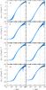 |
Fig. A.1 Radial potential profiles of our simulated galaxies. The black line in each panel shows the potential profile of an NFW sphere with the same virial mass as the galaxy and a concentration c = 10, which was used to define the zero point of the potential. |
In this section we briefly describe how we consistently define the potential in each of
the eight simulations we use in this study. Due to the non-spherical symmetry of the mass
distribution in the simulation box the gravitational potential shows a spread at a given
galactocentric radius. To obtain a robust estimate of the escape speed we redefine the
gravitational potential by assuming that the density profile follows a spherically
symmetric NFW profile (Navarro et al. 1997) beyond
a radius raux:  (A.1)where
ΦNFW is the gravitational potential of an NFW sphere with virial mass
1010 M⊙ and concentration
c′ = 10. The radius raux was
chosen large enough that the approximation of an NFW sphere is well justified, but small
enough that the angular variation of the potential is still small. Furthermore, there must
not be any satellite galaxy near this radius in any of the simulations. For our suite of
simulations, raux = 80 kpc turned out to be a good choice. The
value of the concentration parameter is arbitrary since the potential profile is
insensitive at large radii for any realistic value of c′.
Figure A.1 shows the potential profiles and the
approximated profile. The dips in the lower envelopes of the potentials are caused by
satellite galaxies orbiting the main halo.
(A.1)where
ΦNFW is the gravitational potential of an NFW sphere with virial mass
1010 M⊙ and concentration
c′ = 10. The radius raux was
chosen large enough that the approximation of an NFW sphere is well justified, but small
enough that the angular variation of the potential is still small. Furthermore, there must
not be any satellite galaxy near this radius in any of the simulations. For our suite of
simulations, raux = 80 kpc turned out to be a good choice. The
value of the concentration parameter is arbitrary since the potential profile is
insensitive at large radii for any realistic value of c′.
Figure A.1 shows the potential profiles and the
approximated profile. The dips in the lower envelopes of the potentials are caused by
satellite galaxies orbiting the main halo.
The spread in the potential reflects the fact that these halos live in an anisotropic environment as well as the triaxial shape of the halos. In our simulations we can translate this spread into a maximum deviation from the local escape speed of about 25 km s-1, which is about 5%. The maximum is 40 km s-1 in simulation D and minimum is 7 km s-1 for simulation A.
All Tables
Virial radii, masses, and velocities after rescaling the simulations to have a circular speed of 220 km s-1 at the solar radius R0 = 8.28 kpc.
All Figures
|
Fig. 1 Maximum likelihood parameter pairs computed from mock velocity samples of different sizes. The dotted lines denote the input parameters of the underlying velocity distribution. The contour lines denote positions where the number density fell to 0.9, 0.5, and 0.05 times the maximum value. |
| In the text | |
|
Fig. 2 Normalized velocity distributions of the stellar halo population in our eight simulations plotted as a function of 1−ν∥/νesc. Only counter-rotating particles that have Galactocentric distances r between 4 and 12 kpc are considered to select for halo particles (see Sect. 3.1) and to match the volume observed by the RAVE survey. To allow a comparison, each velocity was divided by the escape speed at the particle’s position. Different colors indicate different simulations, and for each simulation the ν∥ distribution is shown for four different observer positions. The top bundle of curves shows the mean of these four distributions for each simulation plotted on top of each other to allow a comparison. The profiles are shifted vertically in the plot for better visibility. The gray lines illustrate Eq. (3) with power-law index k = 3. |
| In the text | |
|
Fig. 3 Same as the top bundle of lines in Fig. 2 but
plotted as a function of |
| In the text | |
|
Fig. 4 Median values of the likelihood distributions of the power-law index k as a function of the applied threshold velocity νmin. |
| In the text | |
|
Fig. 5 Distribution of |
| In the text | |
|
Fig. 6 Ratios of the estimated and real virial masses in the eight simulations. For each
simulation, four mass estimates are plotted based on four azimuthal positions of
the Sun in the galaxy. The symbols with error bars represent the estimates based
on the median velocities |
| In the text | |
|
Fig. 7 Rescaled radial velocities, |
| In the text | |
|
Fig. 8 Locations of the stars in our high-velocity sample in the
R-z-plane (left panel) and the
x-y-plane (right panel) as
defined in Fig. 7. Blue and orange symbols
represent RAVE stars and B00 stars, respectively. The error bars show 68% confidence
regions (~1σ). Gray contours show the full RAVE catalog, and the
position of the Sun is marked by a white “⊙”. The dashed lines in both panels mark
locations of constant Galactocentric radius |
| In the text | |
|
Fig. 9 Upper panel: distribution of our high-velocity stars as defined in Fig. 7 in a Hertzsprung-Russell diagram (symbols with blue error bars). For comparison the distribution of all RAVE stars (gray contours) and an isochrone of a stellar population with an age of 10 Gyr and a metallicity of −1 dex (red line) is also shown. The two green symbols represent two stars that were excluded from the samples because of their peculiar locations in this diagram. Lower panel: metallicity distribution of our high-velocity sample (blue histogram). The black histogram shows the metallicity distribution all RAVE stars. |
| In the text | |
|
Fig. 10 Upper panel: distribution of the differences of the distance modulus estimates, μ, by B00 and Binney et al. (2013), divided by their combined uncertainty for a RAVE-B00 overlap sample of 68 stars. With σBeers = 1.3 mag we find a spread of 1σ in the distribution with the median shifted by 0.6σ ≃ 0.9 mag. The gray curve shows a shifted normal distribution. The two red data points mark two stars which were also entering our high-velocity samples. Lower panel: direct comparison of the two distance estimates with 1 − σ error bars. The solid gray line represents equality, while the dashed-dotted line marks equality after reducing the B00 distances by a factor of 1.5. |
| In the text | |
|
Fig. 11 Likelihood distributions of parameter pairs νesc,k (lower panel). The positions of the maximum likelihood pairs are marked with the symbols “×” for the V200 samples and “+” for the V300 samples. Contour lines mark the locations where the likelihood dropped to 10% and 1% of the maximum value. The upper panel shows the likelihood distributions marginalized over the most likely k-interval [2.3, 3.7]. |
| In the text | |
|
Fig. 12 Escape speed estimates and 90% confidence intervals in Galactocentric radial bins. The solid black line shows our best-fitting model. Only the filled black data points were used in the fitting process. The red data point illustrates the result of our “localized” approach. |
| In the text | |
|
Fig. 13 Likelihood distribution resulting from our simple Galaxy model when we leave the halo concentration c (and therefore also VLSR) as a free parameter (blue area) for an NFW profile as halo model (left panel) and an adiabatically contracted NFW profile (right panel). The red contours arise when we add the constraints on c from cosmological simulations: the relation of the mean c for a given halo mass found by Macciò et al. (2008) is represented by the thick dashed orange line. The orange area illustrates the spread around the mean c values found in the simulations. The different shades in the blue and orange colored areas mark locations where the probability dropped to 10%, 1% of the maximum value as do the black contour lines for the combined likelihood distribution. Dotted gray lines connect locations with constant circular speed at the solar radius. |
| In the text | |
|
Fig. 14 Additional constraints on the parameter pairs (M340,c) coming from studies from the literature. The black contours are the same as in Fig. 13. Gnedin et al. (2010) measured the mass interior to 80 kpc from the GC, Xue et al. (2008) within 60 kpc and Kafle et al. (2012) inside 25 kpc. The yellow solid and dotted line separate models for which the satellite galaxy Leo I is on a bound orbit (below the lines) from those where it is unbound. |
| In the text | |
|
Fig. A.1 Radial potential profiles of our simulated galaxies. The black line in each panel shows the potential profile of an NFW sphere with the same virial mass as the galaxy and a concentration c = 10, which was used to define the zero point of the potential. |
| In the text | |
Current usage metrics show cumulative count of Article Views (full-text article views including HTML views, PDF and ePub downloads, according to the available data) and Abstracts Views on Vision4Press platform.
Data correspond to usage on the plateform after 2015. The current usage metrics is available 48-96 hours after online publication and is updated daily on week days.
Initial download of the metrics may take a while.