| Issue |
A&A
Volume 561, January 2014
|
|
|---|---|---|
| Article Number | A76 | |
| Number of page(s) | 18 | |
| Section | Interstellar and circumstellar matter | |
| DOI | https://doi.org/10.1051/0004-6361/201322820 | |
| Published online | 03 January 2014 | |
Four new X-ray-selected supernova remnants in the Large Magellanic Cloud⋆
1 Max-Planck-Institut für extraterrestrische Physik, Postfach 1312, Giessenbachstr., 85741 Garching, Germany
e-mail: This email address is being protected from spambots. You need JavaScript enabled to view it.
2 Institut für Astronomie und Astrophysik Tübingen, Universität Tübingen, Sand 1, 72076 Tübingen, Germany
3 Cerro Tololo Inter-American Observatory, National Optical Astronomy Observatory, Cassilla 603 La Serena, Chile
4 Physics and Astronomy Department, University of New Mexico, MSC 07-4220, Albuquerque, NM 87131, USA
5 University of Western Sydney, Locked Bag 1797, Penrith South DC, NSW 1797, Australia
6 Astronomy Department, University of Illinois, 1002 West Green Street, Urbana, IL 61801, USA
Received: 9 October 2013
Accepted: 19 November 2013
Abstract
Aims. We present a detailed multi-wavelength study of four new supernova remnants (SNRs) in the Large Magellanic Cloud (LMC). The objects were identified as SNR candidates in X-ray observations performed during the survey of the LMC with XMM-Newton.
Methods. Data obained with XMM-Newton are used to investigate the morphological and spectral features of the remnants in X-rays. We measure the plasma conditions, look for supernova (SN) ejecta emission, and constrain some of the SNR properties (e.g. age and ambient density). We supplement the X-ray data with optical, infrared, and radio-continuum archival observations, which allow us to understand the conditions resulting in the current appearance of the remnants. Based on the spatially-resolved star formation history (SFH) of the LMC together with the X-ray spectra, we attempt to type the supernovae that created the remnants.
Results. We confirm all four objects as SNRs, to which we assign the names MCSNR J0508−6830, MCSNR J0511−6759, MCSNR J0514−6840, and MCSNR J0517−6759. In the first two remnants, an X-ray bright plasma is surrounded by very faint [S ii] emission. The emission from the central plasma is dominated by Fe L-shell lines, and the derived iron abundance is greatly in excess of solar. This establishes their type Ia (i.e. thermonuclear) SN origin. They appear to be more evolved versions of other Magellanic Cloud iron-rich SNRs which are centrally-peaked in X-rays. From the two other remnants (MCSNR J0514−6840 and MCSNR J0517−6759), we do not see ejecta emission. At all wavelengths at which they are detected, the local environment plays a key role in their observational appearance. We present evidence that MCSNR J0517−6759 is close to and interacting with a molecular cloud, suggesting a massive progenitor.
Key words: ISM: supernova remnants / Magellanic Clouds / X-rays: ISM
Based on observations obtained with XMM-Newton, an ESA science mission with instruments and contributions directly funded by ESA Member States and NASA.
© ESO, 2014
1. Introduction
The study of supernova remnants (SNRs) is crucial to advance our understanding of many important astrophysical processes. SNRs mark the end point of stellar evolution, and return nucleosynthesis products to the interstellar medium (ISM), enriching it with heavy elements. The tremendous amount of energy (~1051 erg) of supernova (SN) explosions heats the ISM up to X-ray emitting temperature (>106 K) and contributes to the mixing of the freshly-produced elements in the SNR environment. Cosmic rays, another important part of the ISM energy budget, can be accelerated up to 1018 eV in SNR shocks (Bell & Lucek 2001).
Many questions related to SNe remain open. The exact nature of the progenitor of type Ia, i.e. thermonuclear SNe, being either a white dwarf accreting from a companion or a merger of two white dwarves, is hotly debated (e.g. Maoz 2008, and references therein). Core-collapse (CC) SNe mark the death of massive, short-lived stars. The lower limit on the mass of a star undergoing a CC SN is about 8 M⊙, but the exact value remains elusive, and so does the mass range leading to various CC SN subtypes (see Smartt 2009, for a review). From a statistically significant sample of SNRs, we can aim to obtain clues to some of these outstanding questions.
The two flavours of SNe deposit a similar amount of energy in the ISM, producing remnants which are harder to type the older they are. The most secure typing methods are the study of SN optical light echoes (Rest et al. 2005, 2008; infrared light echoes can be used to probe the ISM dust, see e.g. Vogt et al. 2012), the measurement of the nucleosynthesis products in the ejecta (e.g. Hughes et al. 1995), or the association with a neutron star/pulsar wind nebula. These methods work well for relatively young remnants (≲5000 yr), leaving a significant fraction of the SNR population untyped. However, several evolved SNRs have been discovered (in X-rays) in the Magellanic Clouds with an iron-rich, centrally bright emission (Nishiuchi et al. 2001; Hendrick et al. 2003; van der Heyden et al. 2004; Seward et al. 2006; Borkowski et al. 2006; Bozzetto et al. 2013b), naturally leading to their classification as type Ia remnants. In addition, studies of the X-ray and infrared morphologies of SNRs (Lopez et al. 2009; Peters et al. 2013) suggest that, as a class, type Ia and CC SNRs have distinct symmetries: type Ia remnants are more spherical and mirror symmetric than the CC SNRs.
Finally, clues to the type of remnants are provided by the study of the stellar population around the SNRs. High-mass stars (i.e. CC-SN progenitors) are rarely formed in isolation but cluster in OB associations. Chu & Kennicutt (1988) used this method to tentatively type all Large Magellanic Cloud (LMC) remnants known at the time. With the availability of the star formation history (SFH) map of the LMC (Harris & Zaritsky 2009), derived from resolved stellar populations, it is now possible to study the connection between remnants and the age of their parent populations. Badenes et al. (2009) performed such a study on (young) SNRs having secure type Ia or CC classifications. As expected, given the short lifetimes of massive progenitors, they found that all CC SNRs in their sample had SFHs dominated by recent peaks of star formation rate. This appears to be necessary, but not sufficient. Indeed, type Ia SNRs can also be found in star-forming regions, as they showed for N103B (see also Hughes et al. 1995; Lewis et al. 2003) or for SNR 0104−72.3 in the Small Magellanic Cloud (SMC) (Lee et al. 2011). On the other hand, the type Ia SNRs of the (limited) sample of Badenes et al. (2009) are associated with a variety of environments, and future similar studies will provide more insights. We investigate the local SFHs of the new SNRs presented in this work as an additional tool to study the origin of the remnants.
Studies of SNRs in the Milky Way are plagued by the large distance uncertainties of, and interstellar absorption towards, sources in the Galactic plane. On the other hand, the LMC offers an ideal laboratory for such studies: first, the distance towards the LMC, our closest star-forming neighbour, is relatively small and very well studied (e.g. Pietrzyński et al. 2013, and references therein). Second, the moderate inclination angle and small line-of-sight depth of the LMC (e.g. Haschke et al. 2012; Subramanian & Subramaniam 2013) mean that we can assume all LMC sources to be at a very similar distance. Third, the interstellar absorption by gas in the foreground is much smaller towards the LMC than towards the Galactic plane, allowing observations even in the soft X-ray regime, below 1 keV. Finally, a wealth of data is available for the LMC from radio to X-rays, allowing for easier detection and classification of SNRs, which classically exhibit three signatures: thermal X-ray emission in the (0.2–5 keV) band, optical line emission with enhanced [S ii] to Hα ratios, and non-thermal (synchrotron) radio-continuum emission. For all these reasons, we can attempt to discover and study the complete sample of SNRs in the LMC.
XMM-Newton observations log, position, and size of the remnants.
The LMC is particularly rich in SNRs. Badenes et al. (2010) compiled a catalogue of 54 SNRs in the LMC. The bulk of the population was discovered/confirmed by early X-ray and radio surveys (Long et al. 1981; Mathewson et al. 1983), and then regularly increased with the completion of more recent surveys (e.g. with Parkes, Filipovic et al. 1998; ROSAT, Williams et al. 1999a; MCELS, Smith et al. 2005; and ATCA Payne et al. 2008). Although a significant fraction of the SNR population of the LMC should have been discovered, there might still be some fainter and more evolved remnants to be found, and candidates to be confirmed. In particular, SNRs lacking one or two of the conventional signatures are harder to identify. Examples of such SNRs can be found in Klimek et al. (2010), Crawford et al. (2010), Grondin et al. (2012), and Bozzetto et al. (2013a).
We carried out a survey of the inner ~4.5° × 4.5° of the LMC with XMM-Newton (Haberl et al., in prep.). In addition to unraveling the X-ray point source population of the LMC (down to ~2 × 1033 erg s-1) and studying its hot gas content, one of the main goals of the survey is to discover new SNRs and to study those, already confirmed, that have not been observed with a modern X-ray observatory. First results from the survey related to that theme have been presented in Maggi et al. (2012) and Bozzetto et al. (2013b).
In this paper we report the discovery of four new SNRs in the XMM-Newton survey of the LMC. A description of the survey, and of the optical, infrared, and radio observations that we used to study the remnants is given in Sect. 2. The reasons why we selected these sources are presented in Sect. 3, then the data analysis is described in Sect. 4. Results are presented and discussed in Sects. 5 and 6. We summarise the results in Sect. 7. Unless otherwise stated, the errors quoted are at the 90% confidence level. Throughout the paper we assume a distance to the LMC of 50 kpc (Pietrzyński et al. 2013).
2. Observations
2.1. X-ray
The sources presented in this work were discovered in observations performed during the XMM-Newton survey of the LMC (Haberl et al., in prep.; see Sect. 3). For this survey we use the European Photon Imaging Camera (EPIC), comprising a pn CCD imaging camera (Strüder et al. 2001) and two MOS CCD imaging cameras (Turner et al. 2001), as the main instrument. All observations are performed using the same instrumental setting: all cameras are operated in full-frame mode, with the thin and medium optical filter for pn and MOS cameras, respectively.
The data used in this paper have been processed with the XMM-Newton SAS1 version 11.0.1. To screen out periods of high background activity, we applied a threshold of 8 and 2.5 cts ks-1 arcmin-2 on pn and MOS light curves in the 7–15 keV energy band. This yielded various useful exposure times, between ~22 and ~33 ks. Details of the XMM-Newton observations are listed in Table 1.
X-ray source detection is performed on all observations from our XMM-Newton survey (which will be presented in detail in future works), using the SAS task edetectchain applied simultaneously to images in five energy bands (given in Watson et al. 2009, Table 3). The detection lists were primarily used to identify our sample of four SNR candidates (Sect. 3). In addition, we could look for central compact objects (CCOs) and exclude unrelated point sources from the spectrum extraction regions.
2.2. Optical
We made use of data from the Magellanic Clouds Emission Line Survey (MCELS, e.g. Smith et al. 2000). Observations were taken with the 0.6 m Curtis–Schmidt telescope from the University of Michigan/Cerro Tololo Inter-American Observatory (CTIO), in three narrow-band filters ([S ii]λλ6716, 6731 Å, Hα, and [O iii]λ5007 Å), and matching red and green continuum filters. We also included data obtained with the MOSAIC ii camera on the Blanco 4 m telescope at the CTIO. Although only a Hα image is available, the superior angular resolution of the MOSAIC ii data (pixel size of less than 1′′) allow faint filaments to appear sharper.
2.3. Infrared
To study possible emission from our objects, and study their surrounding cold environments traced by infrared emission, we used data from the SAGE survey (Meixner et al. 2006), performed with the Spitzer Space Telescope. We essentially used data from the Multiband Imaging Photometer (MIPS; Rieke et al. 2004) in its 24 μm band. We retrieved the MIPS mosaiced, flux-calibrated (in units of MJy sr-1) images processed by the SAGE team, which have a pixel size of 2.49′′.
2.4. Radio
To investigate radio emission from the sources, we used data from various radio surveys, particularly the 4800 MHz survey by Dickel et al. (2010) and the 1370 MHz survey by Hughes et al. (2007). Both surveys used the Australia Telescope Compact Array (ATCA) in fairly compact configurations to produce half-power beamwidths of 35′′ and 45′′, respectively. Data at both frequencies from a survey using the 64 m Parkes telescope (Haynes et al. 1991; Filipovic et al. 1995) were included in the imaging to improve the sensitivity to the smooth emission from these extended regions. We note that none of these objects was visible on the SUMMS radio survey of the southern sky at 843 MHz (Mauch et al. 2003, 2008).
3. Sample selection
To identify SNR candidates, we first selected all extended X-ray sources from the source detection lists. Then, we checked the mosaic images created by our pipeline to screen out spurious sources (for instance, sources at the outer edge of the detector). The final and most important filtering was to exclude real sources that were not SNRs. We list below extended sources that can be found in the field of the LMC and their main X-ray properties.
-
1.
Superbubbles (SBs) are largediameter (~100 pc, corresponding to ~6.9 ′ in the LMC), optically bright shells filled with hot X-ray emitting gas. These objects are powered by the combined stellar winds of massive stars within the shell, with possible contributions by interior SN explosions. They are quite common in the LMC. For details and references, see e.g. Chu & Mac Low (1990) and Dunne et al. (2001).
-
2.
Galaxy clusters behind the LMC can be observed in our survey, like in the SMC (Haberl et al. 2012). The hot intra-cluster medium produces thermal X-ray emission, with typical temperatures of 2 to 10 keV (Rosati et al. 2002). This is much hotter than the plasma temperatures found in middle-aged and mature SNRs (≲1 keV). Galaxy cluster candidates can therefore be recognised by their distinctive hardness ratios (HRs), the ratios of X-ray counts in various energy bands (Sturm et al. 2013).
-
3.
Hot ISM in the LMC produces diffuse emission on large scales. Knots of higher surface brightness can be misidentified as extended sources, but visual inspection of the mosaic images allows to find such cases easily. Study of the hot gas in the LMC with unprecedented spatial resolution will form the core of a future paper.
In the available observations we identified four sources that i) did not belong to any of the above categories; ii) had X-ray properties (e.g. size and soft emission) typical of SNRs; and iii) had enough counts to allow a meaningful spectral analysis. Other candidates, either fainter or in a more complex region (namely, near 30 Doradus), will be presented in future works. A further reason why we focused first on these four sources is that they were observed earlier, in the first pointings of the LMC survey (which is spread over several XMM-Newton Announcements of Opportunity [AO]). All four objects are concentrated towards the north-west end of the stellar bar.
To designate the sources we follow the Magellanic Cloud Supernova Remnant2 Database nomenclature, which uses identifiers of the form “MCSNR JHHMM−DDMM”. Based on their positions, we assign to the four objects the identifiers MCSNR J0508−6830, MCSNR J0511−6759, MCSNR J0514−6840, and MCSNR J0517−6759. We chose to introduce the names of the objects here to allow an easier description of the analysis. For the same reason we will here and after simply call them “remnants” (and no longer “candidates”). Firm evidence for their classification as SNR is presented in Sect. 5.
4. Data analysis
4.1. X-ray imaging
To study the size and morphology of diffuse emission and to look for spatially-resolved spectral variations, we created images and exposure maps in various energy bands from the filtered event lists. We selected single and double-pixel events (PATTERN = 0 to 4) from the pn detector. Below 0.5 keV, however, only single-pixel events were selected to avoid the higher detector noise contribution from the double-pixel events. From the MOS detectors we selected all single to quadruple-pixel (PATTERN = 0 to 12) events. Masks were applied to filter out bad pixels and columns.
We used three energy bands suited to the analysis of the (mostly thermal) spectra of SNRs. A soft band from 0.3 to 0.7 keV includes strong lines from oxygen; a medium band from 0.7 to 1.1 keV comprises Fe L-shell lines as well as Ne Heα and Lyα lines; and a hard band (1.1–4.2 keV) which includes lines from Mg, Si, S, Ca, Ar, and possibly non-thermal continuum.
We used filter-wheel closed (FWC) data, obtained with the detector shielded from the astrophysical background, to subtract the detector background. We estimated the contribution of detector background in each observation from the count rates in the corner of the images, which were not exposed to the sky. We then subtracted approriately-scaled FWC data from the raw images.
Images from pn and MOS detectors were merged together. In the case of MCSNR J0514−6840, two observations included the source in the field of view, and we merged images from the two datasets together. Next, we performed adaptive smoothing: the sizes of Gaussian kernels were computed at each position in order to reach a signal-to-noise ratio of five, setting the minimum full width at half maximum of the kernels to 20′′. In the end the smoothed images were divided by the corresponding vignetted exposure maps.
With the smoothed, exposure-corrected, and detector background-subtracted images in three bands, we created X-ray “true colour” images of the four objects in our sample. These are shown in Figs. 1 to 4. The analysis of the morphology and size of each remnant is presented in Sect. 5.1.
4.2. X-ray spectral analysis
The effective area of the X-ray telescopes varies with off-axis angle across the source extent. To take that into account we extracted spectra from vignetting-corrected event lists, produced with the SAS task evigweight. Only EPIC-pn spectra were used for the spectral analysis because all four remnants are very faint in the MOS-only images.
Except for MCSNR J0517−6759, the extraction regions were circles including all the X-ray emission. Because of the roughly triangular morphology of MCSNR J0517−6759 (see Sect. 5.1), we manually defined a polygonal region following the remnant’s X-ray emission. We extracted background spectra from adjacent regions, which were chosen to be at a similar off-axis angle and on the same CCD chip as the source. However, we note that all remnants but MCSNR J0511−6759 were located on more than one chip, possibly leading to systematic uncertainties in computing response functions and subtracting the background. Point sources detected in the extraction regions were excised.
EPIC-pn spectra including single and double-pixel events were rebinned using the FTOOLS grppha to have a minimum of 25 counts per bin. This allows the use of the χ2-statistic in XSPEC (Arnaud 1996) version 12.8.0, which we utilised for the spectral analysis.
4.2.1. Background modeling
The spectral analysis of extended sources with low surface brightness requires a careful treatment of the background, both instrumental and astrophysical. It is not desirable to simply subtract a background spectrum extracted from a nearby region, because of the different responses and background contributions associated to different regions, and because of the resulting loss in the statistical quality of the source spectrum. Instead, we explicitly model the background and simultaneously fit the source and background spectra. This technique was already applied in our recent analyses of new LMC SNRs (Maggi et al. 2012; Bozzetto et al. 2013b).
The instrumental background (Lumb et al. 2002; Freyberg et al. 2004) comprises i) a particle-induced component called Quiescent Particle Background (QPB), from the interaction of high-energy particles with the detectors; ii) fluorescence lines emitted by the material in the cameras; and iii) internal electronic noise (dominating below 400 eV).
We used FWC data (Sect. 4.1) to model the instrumental background, as no astrophysical X-ray photons are present in these data. Spectra were extracted from FWC data at the same positions on the detector as the source and background extraction regions for each SNR. We applied the same screening and filtering criteria used for the science (i.e. observational) data to the FWC data, and we used the task evigweight to apply a vignetting correction. Formally, the instrumental background is not subjected to vignetting, which is an effect of the telescope on photons. However, by applying a vignetting correction to the science data, we assign weights to genuine X-ray events as well as to particle background events, since we cannot a priori distinguish the two type of events. Therefore, we need to vignetting-correct the FWC data to make sure that the FWC spectra, used for the modeling of the instrumental background contribution to the science data, have been processed in the same way as the latter. At a given position on the detector, evigweight will assign heavier weights to photons with higher energies, an effect that can be easily accounted for in our background model.
The empirical model developed by Sturm (2012) was used to describe the FWC spectra. This includes an exponential decay (modified by a spline function), a power law, and a combination of Gaussian lines to account for the electronic noise, QPB, and instrumental lines, respectively. In addition, two smeared absorption edges to the continuum are included. Finally, we added a spline function to model the effect of the vignetting correction, which “overweights” events above 5 keV, if they have been recorded at significant off-axis angles. This model was not convolved to the instrumental response and we used a normalised diagonal response in XSPEC.
The astrophysical background was modeled by the three-component model of Kuntz & Snowden (2010, their Eq. (2)). The temperature of the unabsorbed thermal component associated to the Local Hot Bubble or Solar Wind Charge Exchange emission was fixed to 100 eV (Henley & Shelton 2008). The photon index of the power law used to model the unresolved extragalactic background was fixed to 1.46 (Chen et al. 1997), whilst the temperature of the (absorbed) Galactic halo emission was allowed to vary.
There could also be X-ray (thermal) emission from hot gas in the LMC that should be taken into account to extract the purest information on the SNRs. This does not occur in any case presented here: first, the four SNRs are in a region of the LMC devoid of significant diffuse emission; such emission is seen more south-east of the remnants, close to the LMC bar and around 30 Doradus, showing where most of the LMC hot gas is located. Second, this diffuse emission would be seen as a thermal component (with temperatures kT ~ 0.2–0.3 keV) and would not be spectrally resolved from the Galactic halo emission. Therefore, any LMC-intrinsic background emission would be accounted for by the hot thermal emission in the three-component background model used.
Finally, to account for a possible soft proton contamination (SPC) in the science spectra, we included an additional power law component, not convolved with the instrumental response.
4.2.2. Source emission
To fit the X-ray emission from the remnants, we first used single-temperature models, assuming either collisional ionisation equilibrium (CIE) or non-equilibrium ionisation (NEI). The CIE model used is vapec in XSPEC and makes use of the Astrophysical Plasma Emission Code (APEC). We used the most recent version available (v2.0.2), which includes updated atomic data (Foster et al. 2012). The update of the collisional excitation data of many iron L-shell ions is particularly relevant to our analysis, as we shall see in Sect. 5.2. As NEI model we chose the plane-parallel shock model of Borkowski et al. (2001, vpshock . It features a linear distribution of ionisation ages (τ = net, where ne is the electron density and t the time since the plasma was shocked) which is more realistic than the single-ionisation age often used in analysis of X-ray spectra of SNRs.
The data did not require/allow the use of multi-temperature models. For the spectrum of MCSNR J0514−6840, which has the best photon statistics due to its higher surface brightness/extent and the fact that it is covered in two XMM-Newton observations, we also tried a Sedov model (vsedov in XSPEC; the prefix “v” in the XSPEC names indicates that abundances can vary). This Sedov model (Borkowski et al. 2001) computes the X-ray spectrum of an SNR in the Sedov-Taylor stage of its evolution.
For the Galactic foreground absorption we used a photoelectric absorption model (phabs in XSPEC) at solar metallicity, with cross-sections taken from Balucinska-Church & McCammon (1992). We included an additional absorption column to the SNR components to model absorption by atomic gas in the LMC. The abundance patterns of these components were fixed to that of the LMC, as measured by Russell & Dopita (1992), and the columns NH LMC were a free parameter in the fits. Elemental abundances of the SNR components were also initially fixed to those of Russell & Dopita (1992). We then determined whether the data required different abundance patterns (see the individual description in Sect. 5.2). All abundances are given relative to the solar values as given by Wilms et al. (2000).
We simultaneously fit the FWC and science data extracted from the background and source regions. The detector background model constrained by the FWC data is included in the corresponding science spectrum, fixing the parameters and allowing only a constant factor between the FWC and science spectra. Likewise, the parameters of the astrophysical background and SPC components in the SNR spectra were linked to the corresponding parameters constrained by the science background spectra.
4.3. Optical
We combined all MCELS observations covering the four SNRs and smoothed the flux-calibrated images with a 2′′ Gaussian. We subtracted the corresponding continuum images, thereby removing (most of) the stellar contribution and revealing the faint diffuse emission in its full extent.
A [S ii]/Hα ratio map was produced. To avoid noise where the pixel values in either bands were low or negative (due to over-subtraction of the continuum, particularly around stars), we set the ratio to 0 for these pixels. From this map we could investigate possible strong [S ii]/Hα ratios, which are indicative of shock excitation. (In the case of photoionisation by a stellar UV field, sulphur is brought to higher ionisation stages, reducing the [S ii]/Hα ratio.) A classical threshold is [S ii]/Hα> 0.4 (Mathewson & Clarke 1973), but see discussion and references in Fesen et al. (1985). We used a more conservative criterion of 0.6 to identify regions where the ratio is clearly enhanced. [S ii]/Hα contours around the SNRs are shown in Figs. 1 to 4, and the results described in Sect. 5.1.
5. Results
5.1. Multi-wavelength morphology
We discuss below the morphology of each remnant. We supplement the dominating X-ray emission with data at longer wavelengths. The sizes and centres of the SNRs (all given in J2000 equinox) are listed in Table 1.
MCSNR J0508−6830:
this remnant is the second faintest source in our sample. It emits X-rays chiefly in the medium band (0.7–1.1 keV), with little or no flux in the softer and harder bands, respectively. This suggests the predominance of iron emission and is explored in greater detail in our spectral analysis (Sect. 5.2).
To estimate the size and nominal centre of the X-ray remnant we fit an ellipse to the 0.7–1.1 keV contours. The outer contour was chosen to be 0.26 times the amplitude (peak intensity minus average background intensity). This would enclose 90% of the flux of a Gaussian-distributed profile. Size uncertainties were estimated by changing the outer contours by ±10% of the total amplitude and then re-computing the size of the ellipse. We found a nominal centre of RA = 05h08m49.5s, Dec = −68°30m41s, a semi-major and semi-minor axis of 1.15′ and 0.90′, respectively, and a position angle (PA) of 40° west of north. The uncertainty is 0.1′ in each direction. At the assumed distance of the LMC, this gives an extent of MCSNR J0508−6830 of 16.7( ± 1.5) pc × 13.1( ± 1.5) pc.
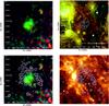 |
Fig. 1 A multicolour view of MCSNR J0508−6830. Top left: X-ray colour image of the remnant, combining the data from all EPIC cameras. The red, green, and blue components are soft, medium, and hard X-rays, as defined in the Sect. 4.1. Top right: the same region of the sky in the light of [S ii] (red), Hα (green), and [O iii] (blue),where all data are from the MCELS. The X-ray contours from the medium band are overlaid. Bottom left: same EPIC image as above but with [S ii]-to-Hα ratio contours from MCELS data. Levels are at 0.6, 0.8, 1.0, and 1.2 in white, cyan, magenta, and red, respectively. Bottom right: the remnant as seen at 24 μm, with the same [S ii]-to-Hα ratio contours as on the left. |
Whilst there is no obvious association in the MCELS images to the X-ray emission, we do detect very faint [S ii] emission, which encircles the remnant seen in X-rays almost completely, except in the south (Fig. 1, top right). At the position of the [S ii] shell there is no contribution from Hα, which is only emitted by the nearby, most likely unrelated, H ii regions. Therefore, this shell and its location around the central X-ray emission appears more clearly in the X-ray image vs. [S ii]/Hα contours (Fig. 1, bottom left). The [S ii] shell is twice as large as the X-ray-emitting region (semi-axes of about 1.9 × 2.0′). We discuss this morphology in light of the spectral results and in comparison with other SNRs in Sect. 6.3.
MCSNR J0508−6830 is not obvious on the radio images but we do see the nearby H ii region to the northeast and curving around to the north and southeast as shown in the optical images. The lack of association of radio emission with the faint [S ii] shell or bright X-ray central region indicates the faintness of the SNR at radio frequencies and/or the insufficient sensitivity of the current radio surveys.
In the infrared, there is no evident emission from the remnant. Most of the diffuse emission of that region (Fig. 1, bottom right) can be associated to the neaby H ii regions seen in radio and in the optical.
MCSNR J0511−6759:
the X-ray colour of this source is very similar to MCSNR J0508−6830, in the sense that the 0.7–1.1 keV band totally dominates the X-ray emission. The morphology is roughly spherical, so we adjusted a circle on the intensity map to derive the position of the centre: RA = 05h11m10.7s, Dec = −67°59m07s. To measure the size and associated uncertainty for the source, we extracted intensity profiles intersecting the remnant’s centre, at ten different position angles. We measured the extent at which the intensity falls below 0.26 times the amplitude (the same criterion as for MCSNR J0508−6830 can be applied as well for this remnant as they have similar morphologies). We repeated this measurement for each PA, before computing the mean and standard deviation of the ten measurements. We obtained a radius of 0.93′± 0.09′, corresponding to a physical size of 13.5( ± 1.3) pc.
In the continuum-subtracted [S ii] images we see faint diffuse emission at the position of MCSNR J0511−6759. This optical emission has a roughly circular morphology, encasing the bright X-ray emission. It appears slightly limb-brightened, indicating a shell morphology, and its extent is ~3.8′ × 3.6′, i.e. larger than the X-ray emission. Hα emission is seen at the same location, albeit even fainter, whilst [O iii]λ5007 Å is completely absent. Despite the faintness of this optical emission, its shell-like morphology and its strong [S ii]/Hα ratio (in excess of 0.6 and reaching 1.5) allows to secure the association of the optical emssion to the X-rays, and to clearly discriminate the remnant from the ambient optical emission, e.g. from the H ii region DEM L89 (Davies et al. 1976) located ~8′ to the north-west. We note the striking similarity of the morphological and spectral features of MCSNR J0511−6759 to those of MCSNR J0508−6830, and refer the reader to the discussion in Sect. 6.3.
In addition, we note the presence of a small knot of X-ray emission, ~1.7′ towards the east, outside of the main X-ray-emitting region. Its morphology is different from that of a point source, and its colour/hardness ratios are very similar to that of the bulk of the X-ray emission. Furthermore, it is located at the eastern tip of the diffuse optical emission described above, suggesting that the knot is likely to belong to the remnant, possibly being a clump of X-ray emitting ejecta (“schrapnel”).
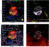 |
Fig. 3 Same as Fig. 1 for MCSNR J0514−6840. On the XMM-Newton image (top left) the 4800 MHz contours are shown in white. Levels are at 1.5, 2, 2.5, and 3 mJy beam-1. The yellow disc in the lower right corner indicates the half-power beamwidth of 35′′. The X-ray contours used on the optical image (top right) are from the soft X-ray image. On the MIPS image (bottom right) the X-ray contours are used to locate the position of the remnant, rather than the (noisy) [S ii]/Hα ratio contours. |
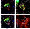 |
Fig. 4 Same as Fig. 1 for MCSNR J0517−6759. On the optical image (top right) we show the soft band X-ray contours in white and the medium band X-ray contours in red. |
MCSNR J0511−6759 was too faint to be detected in the various radio surveys of the LMC. The diffuse infrared emission (at 24 μm) around the remnant is very moderate. A weak filament is found to correlate with the south-eastern part of the [S ii] shell, suggesting a physical association with MCSNR J0511−6759. We discuss a possible origin of this emission in Sect. 6.3.
MCSNR J0514−6840:
unlike the two aforementioned objects, this source has softer colours, being dominated by emission in the 0.3–0.7 keV band. Globally, the morphology is spherically symmetric, although the southern limb is slightly brighter than the northern one. A darker lane also appears to separate the two halves along the east-west equator. Analysis of the X-ray spectrum provide clues to the origin of these features (Sect. 5.2).
Optical emission is present, correlating with the southern edge of the X-ray shell (Fig. 3, top right). Both Hα and [S ii] lines are detected in emission: though the [S ii]/Hα ratio map is still noisy due to the very low diffuse emission of that region, the optical emission at the position of the remnant is clearly in excess of 0.6, indicative of shock-excitation. In addition, [O iii]λ5007 Å emission is present, outlining the edges of the Hα and [S ii]-emitting regions. The strong [O iii] emission suggests partially radiative shocks: when the shock age τ is decreased, the strength of the [O iii] line (relative to Balmer lines) increases, whilst that of [S ii] decreases (see e.g. Dopita et al. 2012, and references therein). The location of the strong [O iii] emission probably traces regions with lower densities and/or shocked more recently.
The position and size of the remnant were obtained from the X-ray image in the same fashion as for MCSNR J0511−6759. We found a centre located at RA = 05h14m15.5s, Dec = −68°40m14s, and a radius of 1.83′ ± 0.12′, i.e. 26.5( ± 1.7) pc.
MCSNR J0514−6840 is the only source of the sample clearly detected at radio frequencies. At 4800 MHz, it looks somewhat like the optical line images with the brightest emission on the southern side. The X-ray image has a more circular outline. The 1370 MHz radio image also seems to have a rather sharp north-south gradient across the whole image near the top of the SNR. The integrated radio flux densities of this SNR are quite uncertain due to the low intensity emission and the relatively high rms noise surrounding this remnant in the radio images. Consequently, it is difficult to obtain an accurate spectral index. However, we estimate that between ν = 843 MHz and ν = 4800 MHz the remnant has a rather flat spectrum with a spectral index α between −0.5 and 0 (defined as S(ν) ∝ να with S(ν) the flux density at frequency ν). The flatter radio-continuum spectrum is indicative of an older remnant.
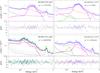 |
Fig. 5 X-ray spectra of the SNRs. Data extracted from the source region are shown by blue data points, with the total (source+background) model as the solid blue line. The red and blue dash-dotted lines show the instrumental background model measured in the background and source extraction regions, respectively. The X-ray+instrumental background model is shown by the dashed red line. For clarity we do not show the data points from the background extraction region but only the residuals of the fit (red points in the lower panels). For MCSNR J0514−6840, spectra from two overlapping observations are shown by the green squares and blue triangles. The thick magenta lines show the source emission component. When more than one component is in the SNR emission model (see text for individual description), the secondary component is shown by the thick green line. The residuals are shown in terms of σ. |
There is no infrared emission that can be clearly linked to the remnant. Bright diffuse emission is seen towards the south of the remnant, indicating a denser/dustier environment in that direction. We explore this further in Sect. 6.1.
MCSNR J0517−6759:
the source exhibits a rather atypical morphology in X-rays, that can be described as “triangular” (Fig. 4). It is elongated along the NE-SW axis with a largest extent of ~5.4′ (78.3 pc). The NE side of the triangle is brighter than the rest of the remnant and extends ~3.5′ (50.8 pc) along the SE-NW direction. This NE “bar” includes all the flux in the medium energy band, whilst the fainter SW “tip” appears softer. As nominal location of the remnant we took the incentre of the triangle delineating the X-ray emission, which yields RA = 05h17m10.2s, Dec = −67°59m03s.
[S ii] and Hα lines are detected in the SW of the remnant, closely following the “tip” of the X-ray emission, with strong [S ii]/Hα ratios (0.6–1.2, see Fig. 4 bottom left). The brighter and harder X-ray “bar” lacks such optical emission. [O iii]λ5007 Å line emission is not observed anywhere in this remnant.
The presence of a point source close to the geometrical centre of MCSNR J0517−6759 is evident in the image (Fig. 4). We identified an infrared/optical counterpart 2.4′′ away from the X-ray source, i.e. well consistent with the typical position uncertainty of XMM-Newton. The counterpart is identified as SAGE J051710.30-675900.9 in the Spitzer catalogue of the LMC (Meixner et al. 2006). Based on its mid-IR colours, it was classified as an active galactic nucleus (AGN) candidate by Kozłowski & Kochanek (2009). Kozlowski et al. (2013) later on spectroscopically confirmed the source as a z = 0.427 AGN. Therefore, we conclude that the central point source in MCSNR J0517−6759 is a background AGN rather than a compact stellar remnant. We discuss later the morphology in greater detail (Sect. 6.1), in light of the X-ray spectroscopy results (Sect. 5.2).
The radio image of MCSNR J0517−6759 only shows weak, compact emission from the central point source, consistent with the AGN classification discussed just above. Bright diffuse 24 μm emission is observed at the south-west of MCSNR J0517−6759. Infrared light intrinsically emitted by the remnant is however likely to be masked by the emission of a nearby molecular cloud (as described in Sect. 6.1). Besides this, two weak filaments outline the eastern and western rims of the remnant. They are presented and discussed in greater detail in Sect. 6.1.
X-ray spectral results.
5.2. X-ray spectroscopy
MCSNR J0508−6830:
the X-ray spectrum of this remnant is shown in Fig. 5, top left. The most striking feature is the large Fe L-shell bump which dominates the X-ray emission.
Despite the faintness of the source, we could obtain meaningful best-fit parameters and uncertainty ranges with the simple spectral models. The results are listed in Table 2. The best fits were obtained for temperatures of about 0.6–0.7 keV and a low absorption, consistent with NH ~ 0 cm-2 (90% C.L. upper limit of 1.8 × 1021 cm-2). We note that for low NH values (≲1021 cm-2), absorption effects are small and mostly affect photons below 0.5 keV. Since the source shows no significant emission below this energy, NH cannot be efficiently constrained. We fixed the LMC NH to 0 cm-2 for the rest of the analysis, stressing that this does not influence the results we present below. No significant effects of non-equilibrium ionisation were detected: the ionisation age was close to the upper limit available in the vpshock model.
The fits greatly improved when the Fe abundance was let free, and improved marginally if O abundance was free as well. The O abundance tended towards 0, but was essentially unconstrained (upper limit of ~20 times the solar value). This happens because at the best-fit temperature (~0.6 keV), which is set by the shape of the iron L-shell bump, the oxygen emissivity is relatively low. We therefore cannot well constrain this parameter. The Fe abundance was found to be greatly in excess of the average LMC value, or even solar value. The upper limit of Fe/Fe⊙ is very high or unconstrained because of the degeneracy between this parameter and the normalisation of the vapec (or vpshock) component. Indeed, since iron is almost the only contributor to the spectrum, the fitting procedure cannot distinguish between a higher iron abundance and lower emission measure, or vice-versa. The low contribution of oxygen to the spectrum and predominance of iron is investigated further in a multi-component plasma analysis (Sect. 5.3).
MCSNR J0511−6759:
the X-ray spectrum of this remnant (Fig. 5, top right) resembles that of MCSNR J0508−6830, as expected from their morphological and X-ray colour similarities. It is also dominated by an Fe L-shell bump and has an even lower contribution from oxygen lines.
The best-fit vapec and vpshock models are obtained for plasma temperatures of 0.64 keV and 0.56 keV, respectively (see Table 2). Initial trial fits were made with a free LMC absorption column. They consistently returned 0 cm-2 as the best-fit value for NH, although the 90% C.L. upper limit of 2.1 × 1021 cm-2 for NH is quite significant. In the rest of the analysis we fixed NH to 0 cm-2 (see the caveat on NH presented above for MCSNR J0508−6830).
Again, no oxygen was formally required, whilst an Fe abundance greatly in excess of the solar value was needed. For the same reason as for MCSNR J0508−6830 we investigated the iron-rich nature of the sourve with a multi-component plasma analysis (Sect. 5.3).
The ionisation age τ in the plane-parallel shock model was high (best-fit value of 8.7 × 10¹¹ s cm-3). Its high 90% C.L. lower limit (1.6 × 10¹¹ s cm-3) and its unconstrained upper limit suggests that the X-ray emitting plasma in MCSNR J0511−6759 is close to or at collisional ionisation equilibrium.
MCSNR J0514−6840:
spectra from the two observations of the source were fit simultaneously. The parameters of the SNR component in both spectra were tied together. The astrophysical background components also shared the same parameters, allowing only for a constant factor between the two sets of spectra. Only the (detector position-dependent) instrumental background and (time-dependent) SPC components had different parameters for each observation.
Good fits were obtained for relatively soft temperatures of 0.2–0.4 keV, depending on the model used (see Table 2). When O and Fe abundances were let free to vary, the fits improved significantly (e.g. χ2/ν = 7979.80/7958 instead of χ2/ν = 8041.68/7960). However, the best-fit values for O/O⊙ and Fe/Fe⊙ were both only reduced by a factor of ~0.6 compared to the value given in Russell & Dopita (1992), being rather consistent with those from Hughes et al. (1998), whilst the ratio O/Fe remained well within the uncertainties of the LMC ISM value given in the two latter references. This indicates that the SN ejecta have no significant contribution to the X-ray spectrum, which is dominated by the swept-up ISM. This justifies a posteriori that the remnant is indeed well in the Sedov phase. It also means that no typing of the SN progenitor can be achieved through the spectral analysis.
We show the X-ray spectrum fitted with the Sedov model in Fig. 5 (bottom left). The formal best-fit parameters with this model are listed in Table 2. The best-fit temperature is rather low and the ionisation age rather high (~2 × 10¹² s cm-3). These two parameters are however relatively poorly constrained. We investigated the kT vs. τ parameter space: equally acceptable fits are allowed both for low temperatures (~0.2 keV) with high ionisation ages (~2 × 10¹² s cm-3), and for higher temperatures (~0.25–0.3 keV) with lower ionisation ages (a few 1011 s cm-3). This degeneracy is explained to some extent to the statistics we have: only lines from a limited set of elements (O, Fe, and possibly Ne) are detected and can be used to constrain those parameters. Another contributor is possibly that the assumption of the Sedov model of a uniform ambient medium does not hold, resulting in asymmetric evolution and varying plasma conditions. The presence of such an inhomogeneous ISM is supported by the optical image, as only the southern edge of the remnant emits lines; as for the X-ray image, the remnant is (marginally) brighter in the southern half.
Guided by the morphology of MCSNR J0514−6840 (Sect. 5.1, Fig. 3), we extracted spectra from the southern and northern halves, in order to look for possible plasma properties or column density (or both) variations across the remnant. In all this analysis, we assumed the ISM to have a homogeneous chemical composition and abundances were fixed at their best-fit values. We divided the SNR along the “dark lane” that crosses the remnant’s equator. First using CIE models, it was possible to constrain the temperature and NH of both spectra, despite the degraded statistics. We found that they had similar temperature (0.18–0.22 keV), but that NH was significantly higher in the south than in the north (~1.3 × 1021 cm-2 vs. ~ 0.3 × 1021 cm-2). Using either the vpshock or Sedov model, we found (roughly five times) higher ionisation ages in the south spectrum as compared to the north, which is again an indication of an inhomogeneous ISM. More specifically, it indicates a density gradient increasing southwards. We interpret these results as environmental effects in Sect. 6.1.
If we assume the Sedov self-similar solution for MCSNR J0514−6840, we can calculate its properties. Given the issues discussed in the above paragraphs, there are concerns that this model, which assumes a spherical symmetry and homogeneous ISM, might yield incorrect results. However, using the best-fit parameters from the integrated spectrum as a measure of the properties averaged over the remnant, we can still obtain rough but useful estimates of important numbers (e.g. age, density, etc.). Alternatively, we can compute the physical properties of the remnant with parameters derived when fitting the north and south spectra, and use these as limiting cases.
The normalisation of the vsedov model is proportional to the volume emission measure  , which can be rewritten as a function of the pre-shock ambient hydrogen density nH,0:
  (1)where RS is the shock radius and r the normalised radius (R/RS). To evaluate the integral one can use the approximation of Kahn (1975) for the normalised mass distribution in the Sedov model (his Eq. (7.19)); numerical integration then gives ≈2.07. Given the radius RS of 26.5 pc and ne/nH ≈ 1.2 (for a fully ionised, 0.5 Z⊙ plasma), we obtain pre-shock densities nH,0 = (0.03 − 0.05) cm-3, using the integrated spectrum. We can then estimate the mass swept-up by the SNR shock as
  , with n0 the ambient pre-shock ion density (≈1.1nH,0) and mp the proton mass. M is in the range (90–150) M⊙.
To estimate the dynamical age of the remnant tdyn, we assume strong shock conditions and full equilibration between electron and ions. Then, the shock velocity vS is related to the X-ray temperature TX by  (2)where k is the Boltzmann constant and μmp is the mean molecular mass (≈0.61mp). The shock velocity is therefore in the range (390–470) km s-1. This is then related to tdyn, the dynamical age of the remnant from Sedov’s similarity relation vS = 2 RS/5tdyn. We found tdyn to be 22–27 kyr. The flatter radio-continuum spectrum is consistent with this quite advanced age. The explosion energy is given by
  , yielding E0 = (0.2 − 0.5) × 1051 erg.
Finally, tion, the age of the remnant derived from the ionisation age τ was about an order of magnitude larger than the dynamical age. The value of τ is however relatively poorly or even not constrained. We note that this can happen if elements contributing to the thermal spectrum are close to CIE. Indeed, as shown by Smith & Hughes (2010), at kT ~ 0.2 keV all astrophysically abundant elements reach ionisation stages close to their equilibrium values on timescales of the order of 1011 s cm-3 to 1012 s cm-3. The non-equilibrium effects in the plasma are therefore small and the ages derived highly uncertain. Values as low as 2 × 10¹¹ s cm-3, which give tion ~ tdyn, are still acceptable within the 3σ uncertainties.
MCSNR J0517−6759:
we started by analysing the integrated spectrum of MCSNR J0517−6759, excluding only the central background AGN. An initial fit with a one-temperature CIE model (vapec) with LMC abundances failed to reproduce the spectrum, as indicated by strong residuals. Namely, the “best-fit” model, with kT ~ 0.5 keV, could reproduce the Fe L-shell emission (between 0.7 and 1.1 keV) but underpredicted the data around 0.5–0.6 keV (dominated by K lines of O vii) whilst predicting too much flux at 0.6–0.7 keV (dominated by the O viii Lyman series). In other words, the temperature constrained by the Fe emission is too high for oxygen. This issue could neither be resolved by using an NEI model, nor by changing the O/Fe abundance balance, because at kT ~ 0.5 keV oxygen is mostly in the H-like ionisation stage (Shull & van Steenberg 1982), and simply increasing the O abundance would overproduce ~0.65 keV emission even more.
Driven by this result and by the morphological analysis of the source (Sect. 5.1), we concluded that a two-temperature model was required. We used two vapec models with distinct temperatures and absorption columns, but both with LMC abundances. This time we obtained satisfactory fits, with no systematic residuals. The integrated spectrum fitted with this model is shown in Fig. 5 (bottom right). Best-fits were obtained with a “hot” (kThot ~ 0.6 keV) and “cool” (kTcool ~ 0.1 keV) component. The hot component models the Fe and O viii emission, whilst the low-temperature component accounts for the extra O vii emission. Although the absorption was poorly determined, the “cool” component required a significantly higher NH (0.6–8.3 × 1021 cm-2) than the “hot” one, which had a best fit-value of ~0 cm-2 and an upper limit of 1.7 × 1021 cm-2. We chose to fix the absorption for the “hot” component to 0 cm-2, whilst for the low-temperature component we fixed the NH to 3.5 × 1021 cm-2, as measured from the H i map of Kim et al. (2003). We give the best-fit parameters of this model and the luminosity of both components in Table 2.
We then proceeded to apply this model to spectra extracted from various regions of the SNR., namely from the NE “bar” and the SW “tip” (Fig. 4). Only normalisations and temperatures of the two components were allowed to change. The best-fit temperatures from the NE and SW spectra were the same as in the integrated spectrum. As expected from the images, we found that ~80% of the flux of the “hot” component is from the NE “bar”, and ≳90% of the “cool” emission is in the SW tip. Scenarios for the origin of this peculiar morphological and spectral features are presented in Sect. 6.1.
5.3. Multi-component plasma fits
The X-ray emission of MCSNR J0508−6830 and MCSNR J0511−6759 is dominated by iron, with a possible minimal contribution from oxygen. To investigate this further, we modeled these sources with a multi-component plasma, each component representing emission from a single element. This approach has been used in the past and allows, under some assumptions, to calculate the mass of the supernova nucleosynthesis products (e.g. Hughes et al. 2003; Kosenko et al. 2010; Bozzetto et al. 2013b).
As initial spectral fits showed (Sect. 5.2), the interior plasma is likely to be in CIE. Consequently, we used vapec models. The abundance of each element in its respective component was set to 109 the solar values, thus making sure we approximate a pure-metal component. Only plasma composed of Fe and O needed to be included in the fit. The temperature of the oxygen plasma (kTO) was not well constrained, given the very small contribution of this element. Therefore, we tied the temperature of this component to that of the Fe component. This is expected if these two elements are co-spatial. We also tried fits with kTO fixed at the peak emissivity temperature of the strongest oxygen lines in the 0.3–1 keV range (i.e. kTO = 0.17 keV). This turned out to have very little influence on the results, which we give for the two remnants in Table 3. The fits returned a zero normalisation of the oxygen component in both MCSNR J0508−6830 and MCSNR J0514−6840, showing the minimal contribution of O in the emission of the two remnants, as expected from the spectral analyses described above.
Results of the multi-component plasma fits for MCSNR J0508−6830 and MCSNR J0511−6759.
The normalisation of each component is proportional to the emission measure EMX (given in terms of nenHV for each component X). Therefore, given a knowledge of the number ratios nX/nH and ne/nX for an element X, we can derive the mass MX of that element produced by the supernova using  (3)(e.g. Kosenko et al. 2010; Bozzetto et al. 2013b), where mU is the atomic mass unit. AX is the atomic mass of element X and VX the volume it occupies. For MCSNR J0511−6759 we assumed a spherical morphology with a radius of 13.5 pc (Sect. 5.1), and therefore VX = 3 × 1059 cm3. The volume of MCSNR J0508−6830 is derived assuming an ellipsoidal morphology, with semi-major and minor axes of 16.7 pc and 13.1 pc. As a third semi-axis we took the average of the two others (i.e. 14.9 pc), yielding VX = 4 × 1059 cm3. This volume would be 13% higher or lower in the case of an oblate or prolate morphology, respectively.
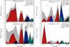 |
Fig. 6 Star formation history around the remnants. Data are taken from Harris & Zaritsky (2009). The star formation rate in four metallicity bins are plotted against lookback time. The errors (combining all metallicities) are shown by the gray shading. The vertical dashed line at 40 Myr indicates the maximal lifetime of a CC SN progenitor. Note the changing vertical scale. |
The main uncertainty for estimating MX is in the ratio of electron-to-ion ne/nX. We follow the prescription of Hughes et al. (2003) and consider two limiting cases. In the first one (case I) the emission originates purely from ejecta, without admixture from hydrogen. Considering that Fe dominates the ejecta, with only minimal contribution from oxygen to the pool of electrons, this means ne/nFe is only set by the average ionisation state of iron. At this temperature we take ne/nFe = 18.3 (Shull & van Steenberg 1982). The second physically plausible case (case II) assumes that a similar mass of H has been mixed with the iron ejecta. Therefore, there are 56 H atoms (contributing each with one electron) per Fe atom, and ne/nFe is 74.3. We give the best-fit parameters and the derived iron mass in both cases in Table 3.
5.4. Local stellar population
We now describe the SFH in the neighbourhood of the four SNRs. We use the spatially resolved SFH map of Harris & Zaritsky (2009). The map was derived from the UBVI photometric survey of Zaritsky et al. (2004) through colour-magnitude diagram fitting. The results are given in terms of star formation rate (SFR, in M⊙ yr-1) in 13 time bins and four metallicity bins, for 1380 cells, most of them having a size of 12′× 12′.
Because stars might drift away from their birth place, one potentially important caveat is that the SFH of a cell hosting a SNR may be derived from stars having no physical connection with the SNR progenitor. For a detailed discussion on the relevance of local stellar populations to the study of progenitors, we point to Badenes et al. (2009). However, we stress that most of the information we can gain from the study of the local SFHs, in the context of broadly typing a remnant, is contained in the most recent time bins. Namely, the presence of recent star formation is a strong necessary (but not sufficient, see the introduction) condition to tentatively type a remnant as having a CC origin. Conversely, the lack of recent star-forming activity favours a thermonuclear origin (see Sect. 6.2).
For each SNR we plot the SFR of the cell including the remnant (Fig. 6), as a function of lookback time and metallicity. MCSNR J0508−6830 and MCSNR J0514−6840 are located in the region coined “outer bar” by Harris & Zaritsky (2009), and they share some properties: the SFR is moderate in the recent past and is declining at times t < 50 Myr. The quiescence periods at 250 Myr and 1 Gyr are rather deep. The SFR around MCSNR J0514−6840 has its stronger peaks at ~500 Myr and 1.6 Gyr, whilst MCSNR J0508−6830 exhibits an even stronger peak at 100 Myr.
MCSNR J0511−6759 and MCSNR J0517−6759 reside in the “Northwest void” region of Harris & Zaritsky (2009), characterised by a low SFR throughout all epochs and no significant enhanced star formation activity period (note the different vertical axis scale of the SFH plots). However, the cell including MCSNR J0517−6759 shows a strong peak at 12 Myr. We checked the neighbouring cells to find that this recent SFR enhancement is concentrated around the remnant rather than being a larger scale feature. MCSNR J0517−6759 is the only remnant of the sample whose SFH is dominated by a burst of recent star formation.
6. Discussion
With these four new objects, the SNR population of the LMC now amounts to more than 60 (Badenes et al. 2010; Grondin et al. 2012; Maggi et al. 2012; Kavanagh et al. 2013; Bozzetto et al. 2013a,b). The SNRs have sizes in the upper range of the distribution of diameter of LMC SNRs (Badenes et al. 2010), as expected from their fairly advanced evolutionary stage.
The non-detection in radio of three out of four objects (namely, MCSNR J0508−6830, MCSNR J0511−6759, and MCSNR J0517−6759) is rare for LMC SNRs, as all known remnants either show radio-continuum emission (e.g. Badenes et al. 2010) or available observations are impacted by bright objects in the remnants’ neighbourhood. This lack of detection would imply old remnants, with ages in excess of 20–30 kyr. In these cases the SNRs become very faint, and coupled with the likely low density environment in which they reside, it is not surprising that we are unable to detect them at any radio frequencies. Future radio-continuum observations in this lower frequency range, potentially with the Murchison Widefield Array (MWA, Tingay et al. 2013), may be able to detect such faint emission.
We now discuss the most interesting features of each remnant, namely: for MCSNR J0514−6840 and MCSNR J0517−6759, the observed effect of an inhomogeneous ISM; for all four SNRs, the type of SN origin; for MCSNR J0508−6830 and MCSNR J0511−6759, the iron-rich nature.
6.1. Environmental effects and asymmetric evolution
MCSNR J0514−6840 displays a subtle variation of X-ray colour along its north-south axis (Fig. 3), being harder towards the south. The X-ray spectral analysis in Sect. 5.2 strongly suggests that this is a foreground extinction effect by a varying absorption column density. The higher NH of the southern half suppresses more soft X-ray flux than in the northern half, resulting in the observed colour gradient.
Direct evidence for the north-south density gradient can be found at longer wavelengths, e.g. in the H i map of Kim et al. (2003, Fig. 7. The Spitzer MIPS 24 μm image of the neighbourhood of the remnant (Fig. 3), which traces cold dust, also shows a dustier environment towards the south. It is reasonable to postulate that the X-ray dark lane seen across the remnant is also a consequence of foreground absorption, although the obscuring structure falls below the spatial resolution of the H i map.
MCSNR J0517−6759 exhibits a more dramatic asymmetry: a cool (~0.1 keV) X-ray shell is seen in the SW, correlating with relatively bright Hα and [S ii] emission. In the NE, we see a “ridge” of X-ray emission with higher temperature (~0.6 keV) and little to no co-spatial optical emission.
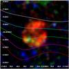 |
Fig. 7 X-ray image of MCSNR J0514−6840 overlaid with H i column density contours. Levels shown are 1.5, 1.75, 2.0, 2.25, and 2.5, in units of 1021 cm-2, increasing from north to south. |
To provide a better view of the remnant’s emission at various wavelengths, we show in Fig. 8 an annotated triptych of MCSNR J0517−6759 as seen at 24 μm and in Hα and [S ii] lines. Mid-IR point sources within the remnant are the background AGN discussed in Sect. 5.1 (cyan circle “A” in Fig. 8) and a B = 14.75 mag star identified as 2MASS J05170629-6758401 (Zaritsky et al. 2004; Skrutskie et al. 2006). The star is likely to simply lie in projection within MCSNR J0517−6759 and to be unrelated to the remnant. However, the ionising radiation of 2MASS J05170629-6758401 is responsible for the compact H ii region around the star that is seen in optical lines (green circle “C” in Fig. 8) and might hide actual SNR emission. In spite of these interlopers, it is possible to see faint filaments in optical lines, identified by the “S1” and “S2” ellipses in Fig. 8, which connect the bright optical arc in the SW to the X-ray ridge in the NE. 24 μm emission is also seen in these filaments, possibly originating from compressed, heated dust in the pre-shock region. Since the temperature is so low (almost too cool to emit X-rays), line emission by [O iv] (at 25.9 μm) is also likely contributing to the MIPS data. Only the X-ray ridge remains not enclosed by longer wavelength emission.
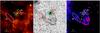 |
Fig. 8 Annotated view of MCSNR J0517−6759, as seen at 24 μm (left) and in the lines of Hα (middle) and [S ii] (right). The Hα image has been taken with the Blanco 4-m telescope and have a pixel size of 0.27′′ × 0.27′′ (no continuum has been subtracted). The ellipses (“S1” and “S2”) mark faint filaments (see Sect. 6.1 for details). The green circle (“C”) shows an unrelated compact H ii region, and the cyan circle (“A”, left image) marks the background AGN detected in X-rays and in the mid-IR. |
We again postulate that the asymmetry is essentially governed by the inhomogeneous ISM. Several tracers indicate a much denser ISM towards the SW of the remnant, namely:
-
1.
atomic hydrogen (Kimet al. 2003), see contours inFig. 9.
-
2.
CO emission; MCSNR J0517−6759 is located at the NE boundary of the giant molecular cloud (GMC) [FKM2008] LMC N J0516-6807 (Fukui et al. 2008, green contours in Fig. 9). We stress that the NANTEN survey only has moderate resolution3 (beam size of 2.6′). The green contours in Fig. 9 are somewhat misleading, as the brightest part of the GMC (i.e. where most of the molecular material resides) is really towards the SW, in the same direction as the elongation of the SNR.
-
3.
Cold dust; Mid-IR emission (24 μm) outlines the outer part of the GMC (can be seen in Fig. 8).
As Lopez (2013) shows, SNRs interacting with molecular clouds are the most elliptical (or elongated) remnants. In the presence of high density inclusions, the SNR blast wave is slowed, and consequently the remnant loses its spherical structure or intrinsic (a)symmetries early in its evolution. MCSNR J0517−6759 exemplifies the key role of environment on shaping the morphology of evolved SNRs.
The evolution of SNRs expanding in a non-uniform ISM has been investigated by several authors in numerical simulations (e.g. Dohm-Palmer & Jones 1996; Hnatyk & Petruk 1999; Orlando et al. 2009), pointing to the asymmetries that develop along the density gradient. However, these studies dealt with much younger SNRs than MCSNR J0517−6759. In particular, Hnatyk & Petruk (1999) showed the strong X-ray surface brightness contrast that can be produced by density gradients. The brightest emission is expected from the densest region, as LX scales with the square of the density. This effect likely contributes to the slightly brighter emission in the south of MCSNR J0514−6840, but we see the opposite trend in the case of MCSNR J0517−6759, which shows brighter emission from the lower density region. This can be interpreted as a later-time evolution effect: the interaction of the blast wave with the much denser ISM in the SW caused the shock to cool down quickly and to become radiative, leading to a lower level of X-ray emission. The X-rays emitted are also softer and more easily absorbed (especially since NH is larger in the SW), further reducing the observed X-ray flux. This scenario also explains the stronger optical emission in the SW.
The low-temperature component in the SW is seen essentially as a line complex at 0.5–0.6 keV. There could be charge exchange (CX) emission contribution to that line complex, instead of a purely thermal emission. CX X-ray emission in SNRs has been detected in the Cygnus Loop and Puppis A remnants (Katsuda et al. 2011, 2012). The fraction of CX to the X-ray emission can be enhanced if the hot gas is interacting with denser, neutral gas, as we suggest for MCSNR J0517−6759. However, the data available allow neither to rule out the presence, nor to constrain the contribution of CX to the X-ray emission of the cool SW shell.
The NE part of the blast wave, on the other hand, expands in a more tenuous environment and is seen as the X-ray ridge. The higher shock temperature (or expansion velocity) in the lower density region is consistent with the results of Dohm-Palmer & Jones (1996). As a consequence of the bi-lateral velocity structure, the apparent centre of the remnant shifts away from the actual explosion site, towards the lower-density region. The shifts predicted by Dohm-Palmer & Jones are up to 20% of the apparent radius. The SN that created MCSNR J0517−6759 should conversely have exploded south-west of the apparent geometrical centre, i.e. more embedded within the molecular cloud [FKM2008] LMC N J0516-6807. This makes the case for a massive stellar progenitor more likely (see Sect. 6.2).
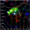 |
Fig. 9 Same as Fig. 7 for MCSNR J0517−6759, with CO contours from the NANTEN survey added in green. The H i levels shown are 2.0, 2.25, 2.5, and 2.75 (in units of 1021 cm-2), in white, cyan, magenta, and red, respectively. CO contours are from 1σ to 5σ, in steps of 1σ (≈0.4 K km s-1), and increase westwards. |
An alternative explanation might be that the SNR shock broke out into the lower-density medium in the NE, as suggested for e.g. N11L and N86 (Williams et al. 1999b). However, the higher temperature of the plasma in the breakout region and the current lack of detected optical filaments “streaming” ahead of the breakout are at odds with this scenario. It is also possible that MCSNR J0517−6759 is similar to e.g. DEM L238, DEM L249, or MCSNR J0508-6902 (Borkowski et al. 2006; Bozzetto et al. 2013b): the X-ray “ridge” is actually at the centre of the SNR shell but only the SW part of the shell remained detectable. Unless deeper data are available, any scenario will remain highly speculative and we favour the simpler scenario of “asymmetric evolution” described above.
6.2. Typing the SNRs
MCSNR J0508−6830 and MCSNR J0511−6759 are iron-rich, as revealed by the X-ray analysis (Sect. 5.2). Under the assumption that the emission is composed primarily of ejecta, we derived in Sect. 5.3 that a large mass of iron – between 0.5 M⊙ and 1.2 M⊙, depending on the level of hydrogen mixing – has been produced in these SNe. However large the uncertainties, these results clearly favour a type Ia SN origin for MCSNR J0508−6830 and MCSNR J0511−6759. Indeed, thermonuclear SNe produce much more iron than CC SNe (e.g. Iwamoto et al. 1999). The nucleosynthesis yield of CC SNe, on the other hand, peaks for oxygen and subsequent α-group elements (i.e. Ne, Mg, see e.g. Woosley & Weaver 1995). Therefore, the large Fe/O ratio observed is also arguing against a CC SN origin.
No ejecta emission is detected from MCSNR J0514−6840 and MCSNR J0517−6759, making the study of the remnants’ environment the only path to a tentative typing of their parent SNe. We attempt to quantify r = NCC/NIa, the ratio of CC SNe to thermonuclear SNe expected from the observed distribution of stellar ages in the neighbourhood of the remnants.
Over the visibility time of a remnant – taking 100 kyr as a very conservative limit – the stars in the SFH cell including the remnant will not drift away. In other words, the distribution of stellar ages observed now is the same as that when the SN exploded. We used the delay time distribution Ψi(τ), the SN rate at time τ following a star formation event, measured by Maoz & Badenes (2010) in the Magellanic Clouds, with i = 1, 2, and 3 designating the time intervals they used (t < 35 Myr, 35 Myr < t < 330 Myr, and 330 Myr < t < 14 Gyr, respectively). From timescale arguments it is reasonable to assume that Ψ1 will correspond to the CC SN rate, whilst Ψ2 and Ψ3 will be that of SNe Ia (regardless of their “prompt” or “delayed” nature). We can integrate the SFR to obtain Mi, the stellar mass formed in each time interval. Then, we can compute r as the ratio of the rates of CC and Ia SNe, since the visibility times are the same for both types, leading to: 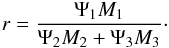 (4)The SFHs around MCSNR J0508−6830 and MCSNR J0511−6759 (Sect. 5.4) lack a significant peak of recent (less than 40 Myr) star formation activity, which translates into rather small r values of 1.4 and 0.6, respectively, for these remnants. A similar value (r = 1.4) is obtained for MCSNR J0514−6840, as expected given the similarities of the SFHs of MCSNR J0508−6830 and MCSNR J0514−6840. Finally, for MCSNR J0517−6759, we derived a much higher ratio of r = 7.6.
Intuitively, any value r > 1 should favour a CC SN origin (conversely for a thermonuclear origin). However, an important caveat to interpret these results is that the rates of Maoz & Badenes (2010), especially Ψ2 and Ψ3, are quite uncertain, due to the still limited sample of SNRs. Specifically, Ψ2 has a value that changes by a factor of four depending on the tracer used to constrain the SNR visibility time. (Here we adopted Ψ2 = 0.26 SNe yr-1 (1010M⊙)-1 and Ψ3 < 0.0014 SNe yr-1 (1010M⊙)-1. Note that because Ψ3 is an upper limit, r is formally a lower limit.)
To provide a better feeling on what r value to expect in either case, we derived this ratio for SNRs having a well secured type. We took the sample of four CC and Ia SNRs of Badenes et al. (2009). For type Ia remnants, we obtained r = 2.2, 0.9, and 1.0 for DEM L71, SNR 0509-67.5, and SNR 0519-69.0, respectively. N103B has r = 3.2 but is atypical, as it is in a star forming region. Core-collapse SNRs have r ranging from 2.6 (N49) to more extreme values (e.g. r = 21.7 for N158A).
In spite of large uncertainties, the ratio r = NCC/NIa still appears as a useful tool to assign a type to SNRs using the observed local SFH. It provides a quantitative criterion to confirm the intuition that SNR without a prominent peak of recent star formation are more likely to originate from a type Ia SN. Values in excess of 2 favour a CC scenario, whilst type Ia SNRs will exhibit r ≲ 1. r ≫ 2 or ≪1 allow more secure typing in either ways. Intermediate value (between 1 and 2) lead to uncertain classification, though preliminary results (e.g. for MCSNR J0508−6830) show that a type Ia remnant can have r = 1.4.
To conclude, this analysis makes the case for a type Ia origin of MCSNR J0508−6830 and MCSNR J0511−6759 even stronger. MCSNR J0517−6759 is the only source having a prominent peak of recent star formation. The large r value of 7.6 strongly argues for a CC SN origin of MCSNR J0517−6759. The asymmetric/elongated morphology, likely originating from the interaction with a molecular cloud, with which the remnant is associated (Sect. 6.1), is consistent with this type (Lopez 2013). Finally, we marginally favour a thermonuclear origin MCSNR J0514−6840. We stress, however, that the classification of this remnant is more uncertain than for the other objects, for which other clues to the SN type are available.
6.3. Two iron-rich SNRs
MCSNR J0508−6830 and MCSNR J0511−6759 are remarkable in their morphological and chemical structure. The centrally located iron-rich plasma betray their type Ia SN origin. They join the sample of MC SNRs with a faint, soft X-ray shell containing iron-rich hot gas in collisional equilibrium (see references in the Introduction). They are likely more evolved versions of the very similar remnants DEM L238, DEM L249, and MCSNR J0508−6902. The main difference with these is the absence in our data of a detected X-ray shell, whilst very dim [S ii] emission still indicates the locations of the furthest advance of the SN blast wave. This echoes other cases in the SMC, namely DEM S128, IKT 5, and IKT 25 (van der Heyden et al. 2004). The faint sulphur emission and lack of soft X-rays from the shells of MCSNR J0508−6830 and MCSNR J0511−6759 indicate that they reached the point when radiative cooling caused the shells to become either too cool to emit X-rays, or too faint to be detected in the data available. Another possibility is a compositional difference, with Fe in centre and more normal composition outside which would make for a high emissivity contrast at a given thermal pressure. If the temperature in the shell is that low, we might expect [O iv] emission at 25.9 μm. The detection of faint filament in the MIPS image, at the south-eastern rim of the [S ii] shell of MCSNR J0511−6759, lends support to that scenario.
As discussed in Borkowski et al. (2006), the long ionisation ages of the iron-rich central plasma is puzzling given the type Ia classification of these remnants, because it requires higher densities in the centre than expected from standard type Ia SN models. A possibility is that the SN progenitor was more massive (~3 to 8 M⊙) than average, because the stellar winds of these “prompt” progenitors increase the circumstellar density.
The central location of most of the X-ray emission is reminiscent of the mixed-morphology SNRs classification (MMSNRs, Rho & Petre 1998; Lazendic & Slane 2006), which has been applied only to Galactic remnants. The MMSNRs are usually close to, and interacting with, a molecular cloud environment, showing OH masers. It means that the MMSNRs very likely have massive progenitors and are not type Ia SNRs, as we conclude for MCSNR J0508−6830 and MCSNR J0511−6759.
The number of known iron-rich SNRs with centrally-peaked in X-rays has significantly increased thanks to the XMM-Newton survey of the LMC (Bozzetto et al. 2013b, this work). We have access to a sample of evolved remnants which cannot be studied in the Milky Way, because the high column density towards the Galactic plane, (much) in excess of 1022 cm-2, readily absorbs most or all the photons below 1 keV. As such, all iron lines are hidden (there is no Fe K emission at these temperatures). Unfortunately, because MCSNR J0508−6830 and MCSNR J0511−6759 are (relatively) X-ray dim and have only been observed in short or moderately long exposures, the data currently available suffer from low statistics, which is further reduced by the off-axis location of the source in the survey observations. Deeper observations with the current X-ray telescopes or future instrumentation (e.g. Athena+, Decourchelle et al. 2013) are warranted to yield higher-quality images and spectra. This will enable, e.g., more accurate measurements of the physical conditions in the plasma, of abundances, or allow to look for spectral variations across the remnants.
7. Summary
We have presented four new members of the LMC SNR population, discovered in the survey performed with XMM-Newton. All four are relatively evolved remnants. Their thermal X-ray emission is the key signature of their nature, although observations at longer wavelengths are essential to understand the conditions resulting in their current appearance. Our analysis concluded that:
-
1.
MCSNR J0508−6830 andMCSNR J0511−6759 are iron-rich,centrally-peaked in X-rays SNRs. They are spectrally verysimilar to DEM L238, DEM L249,and MCSNR J0508-6902, although they have nodetected shell around the central iron-rich plasma. However,faint [S ii] emission surrounding them is likely arelic of the propagation of the SN blast wave. From X-ray spectralfits, we measure the presenceof (0.5–1) M⊙ and (0.6–1.2) M⊙ of Fe in MCSNR J0508−6830 and MCSNR J0511−6759, respectively. The large amounts of iron in the SNR interiors and the lack of recent star formation in the neighbourhood of the remnants both strongly point to a type Ia SN origin.
-
2.
MCSNR J0514−6840 is a large diameter (53 pc), roughly spherically symmetric remnant, whose X-ray spectrum is entirely from the shocked ISM. It displays optical emission coextensive with the X-rays in the southern half of the remnant. MCSNR J0514−6840 is the only object of our sample to be detected at radio frequencies, just above the noise limit, and only from the southern half. This indicates that radio emission from the other remnants, if present, is too faint to be detected in currently available data. The north-south asymmetry of the radio and optical emission is interpreted as a non-uniform ambient medium, having a density increasing towards the south. The X-ray-derived NH in the southern half of the remnant is indeed higher than in the northern one, in keeping with the NH gradient seen in the H i map of the LMC, lending support to our interpretation.
-
3.
MCSNR J0517−6759 exhibits a very unusual morphology. A very soft X-ray shell in the south-west is closed by a harder X-ray “bar” in the north-east. Optical emission with high [S ii]/Hα correlates only with the soft X-rays in the south-west, where a giant molecular cloud is reported. This leads us to the interpetation that the SN blast wave is propagating into a much denser ISM towards the south-west. There, the shock quickly slowed and cooled down, producing the very soft X-rays, whilst being relatively unperturbed towards the north-east. The association with a molecular cloud and the recent star formation in the local SFH suggest a massive progenitor for MCSNR J0517−6759.
Science Analysis Software, http://xmm.esac.esa.int/sas/
None of our objects are fully covered by the MAGMA survey of the LMC (Wong et al. 2011), which has a higher angular resolution (~45′′).
Acknowledgments
The XMM-Newton project is supported by the Bundesministerium für Wirtschaft und Technologie/Deutsches Zentrum für Luft- und Raumfahrt (BMWi/DLR, FKZ 50 OX 0001) and the Max-Planck Society. Cerro Tololo Inter-American Observatory (CTIO) is operated by the Association of Universities for Research in Astronomy Inc. (AURA), under a cooperative agreement with the National Science Foundation (NSF) as part of the National Optical Astronomy Observatories (NOAO). We gratefully acknowledge the support of CTIO and all the assistance which has been provided in upgrading the Curtis Schmidt telescope. The MCELS is funded through the support of the Dean B. McLaughlin fund at the University of Michigan and through NSF grant 9540747. We used the karma software package developed by the ATNF. The Australia Telescope Compact Array is part of the Australia Telescope which is funded by the Commonwealth of Australia for operation as a National Facility managed by CSIRO. P.M. and P.K. acknowledge support from the BMWi/DLR grants FKZ 50 OR 1201 and 50 OR 1209, respectively. M.S. acknowledges support by the Deutsche Forschungsgemeinschaft through the Emmy Noether Research Grant SA 2131/1. This research has made use of Aladin, SIMBAD and VizieR, operated at the CDS, Strasbourg, France.
References
- Arnaud, K. A. 1996, in Astronomical Data Analysis Software and Systems V, eds. G. H. Jacoby, & J. Barnes, ASP Conf. Ser., 101, 17 [Google Scholar]
- Badenes, C., Harris, J., Zaritsky, D., & Prieto, J. L. 2009, ApJ, 700, 727 [NASA ADS] [CrossRef] [Google Scholar]
- Badenes, C., Maoz, D., & Draine, B. T. 2010, MNRAS, 407, 1301 [NASA ADS] [CrossRef] [Google Scholar]
- Balucinska-Church, M., & McCammon, D. 1992, ApJ, 400, 699 [NASA ADS] [CrossRef] [Google Scholar]
- Bell, A. R., & Lucek, S. G. 2001, MNRAS, 321, 433 [NASA ADS] [CrossRef] [Google Scholar]
- Borkowski, K. J., Lyerly, W. J., & Reynolds, S. P. 2001, ApJ, 548, 820 [NASA ADS] [CrossRef] [Google Scholar]
- Borkowski, K. J., Hendrick, S. P., & Reynolds, S. P. 2006, ApJ, 652, 1259 [NASA ADS] [CrossRef] [Google Scholar]
- Bozzetto, L. M., Filipović, M. D., Crawford, E. J., et al. 2013a, MNRAS, 432, 2177 [NASA ADS] [CrossRef] [Google Scholar]
- Bozzetto, L. M., Kavanagh, P. J., Maggi, P., et al. 2013b, MNRAS, submitted [Google Scholar]
- Chen, L.-W., Fabian, A. C., & Gendreau, K. C. 1997, MNRAS, 285, 449 [NASA ADS] [CrossRef] [Google Scholar]
- Chu, Y.-H., & Kennicutt, Jr., R. C. 1988, AJ, 96, 1874 [NASA ADS] [CrossRef] [Google Scholar]
- Chu, Y.-H., & Mac Low, M.-M. 1990, ApJ, 365, 510 [NASA ADS] [CrossRef] [Google Scholar]
- Crawford, E. J., Filipović, M. D., Haberl, F., et al. 2010, A&A, 518, A35 [NASA ADS] [CrossRef] [EDP Sciences] [Google Scholar]
- Davies, R. D., Elliott, K. H., & Meaburn, J. 1976, Mem. Roy. Astron. Soc., 81, 89 [Google Scholar]
- Decourchelle, A., Costantini, E., Badenes, C., et al. 2013 [arXiv:1306.2335] [Google Scholar]
- Dickel, J. R., McIntyre, V. J., Gruendl, R. A., & Milne, D. K. 2010, AJ, 140, 1567 [NASA ADS] [CrossRef] [Google Scholar]
- Dohm-Palmer, R. C., & Jones, T. W. 1996, ApJ, 471, 279 [NASA ADS] [CrossRef] [Google Scholar]
- Dopita, M. A., Payne, J. L., Filipović, M. D., & Pannuti, T. G. 2012, MNRAS, 427, 956 [NASA ADS] [CrossRef] [Google Scholar]
- Dunne, B. C., Points, S. D., & Chu, Y.-H. 2001, ApJS, 136, 119 [NASA ADS] [CrossRef] [Google Scholar]
- Fesen, R. A., Blair, W. P., & Kirshner, R. P. 1985, ApJ, 292, 29 [NASA ADS] [CrossRef] [Google Scholar]
- Filipovic, M. D., Haynes, R. F., White, G. L., et al. 1995, A&AS, 111, 311 [NASA ADS] [Google Scholar]
- Filipovic, M. D., Haynes, R. F., White, G. L., & Jones, P. A. 1998, A&AS, 130, 421 [NASA ADS] [CrossRef] [EDP Sciences] [Google Scholar]
- Foster, A. R., Ji, L., Smith, R. K., & Brickhouse, N. S. 2012, ApJ, 756, 128 [NASA ADS] [CrossRef] [Google Scholar]
- Freyberg, M. J., Briel, U. G., Dennerl, K., et al. 2004, in SPIE Conf. Ser. 5165, eds. K. A. Flanagan & O. H. W. Siegmund, 112 [Google Scholar]
- Fukui, Y., Kawamura, A., Minamidani, T., et al. 2008, ApJS, 178, 56 [NASA ADS] [CrossRef] [Google Scholar]
- Grondin, M.-H., Sasaki, M., Haberl, F., et al. 2012, A&A, 539, A15 [NASA ADS] [CrossRef] [EDP Sciences] [Google Scholar]
- Haberl, F., Sturm, R., Ballet, J., et al. 2012, A&A, 545, A128 [NASA ADS] [CrossRef] [EDP Sciences] [Google Scholar]
- Harris, J., & Zaritsky, D. 2009, AJ, 138, 1243 [NASA ADS] [CrossRef] [Google Scholar]
- Haschke, R., Grebel, E. K., & Duffau, S. 2012, AJ, 144, 106 [NASA ADS] [CrossRef] [Google Scholar]
- Haynes, R. F., Klein, U., Wayte, S. R., et al. 1991, A&A, 252, 475 [NASA ADS] [Google Scholar]
- Hendrick, S. P., Borkowski, K. J., & Reynolds, S. P. 2003, ApJ, 593, 370 [NASA ADS] [CrossRef] [Google Scholar]
- Henley, D. B., & Shelton, R. L. 2008, ApJ, 676, 335 [NASA ADS] [CrossRef] [Google Scholar]
- Hnatyk, B., & Petruk, O. 1999, A&A, 344, 295 [NASA ADS] [Google Scholar]
- Hughes, J. P., Hayashi, I., Helfand, D., et al. 1995, ApJ, 444, L81 [NASA ADS] [CrossRef] [Google Scholar]
- Hughes, J. P., Hayashi, I., & Koyama, K. 1998, ApJ, 505, 732 [NASA ADS] [CrossRef] [Google Scholar]
- Hughes, J. P., Ghavamian, P., Rakowski, C. E., & Slane, P. O. 2003, ApJ, 582, L95 [NASA ADS] [CrossRef] [Google Scholar]
- Hughes, A., Staveley-Smith, L., Kim, S., Wolleben, M., & Filipović, M. 2007, MNRAS, 382, 543 [NASA ADS] [CrossRef] [Google Scholar]
- Iwamoto, K., Brachwitz, F., Nomoto, K., et al. 1999, ApJS, 125, 439 [NASA ADS] [CrossRef] [MathSciNet] [Google Scholar]
- Kahn, F. D. 1975, in Int. Cosmic Ray Conf., 11, 3566 [Google Scholar]
- Katsuda, S., Tsunemi, H., Mori, K., et al. 2011, ApJ, 730, 24 [NASA ADS] [CrossRef] [Google Scholar]
- Katsuda, S., Tsunemi, H., Mori, K., et al. 2012, ApJ, 756, 49 [NASA ADS] [CrossRef] [Google Scholar]
- Kavanagh, P. J., Sasaki, M., Points, S. D., et al. 2013, A&A, 549, A99 [NASA ADS] [CrossRef] [EDP Sciences] [Google Scholar]
- Kim, S., Staveley-Smith, L., Dopita, M. A., et al. 2003, ApJS, 148, 473 [NASA ADS] [CrossRef] [Google Scholar]
- Klimek, M. D., Points, S. D., Smith, R. C., Shelton, R. L., & Williams, R. 2010, ApJ, 725, 2281 [NASA ADS] [CrossRef] [Google Scholar]
- Kosenko, D., Helder, E. A., & Vink, J. 2010, A&A, 519, A11 [NASA ADS] [CrossRef] [EDP Sciences] [Google Scholar]
- Kozłowski, S., & Kochanek, C. S. 2009, ApJ, 701, 508 [NASA ADS] [CrossRef] [Google Scholar]
- Kozlowski, S., Onken, C. A., Kochanek, C. S., et al. 2013, ApJ, 775, 92 [NASA ADS] [CrossRef] [Google Scholar]
- Kuntz, K. D., & Snowden, S. L. 2010, ApJS, 188, 46 [NASA ADS] [CrossRef] [Google Scholar]
- Lazendic, J. S., & Slane, P. O. 2006, ApJ, 647, 350 [NASA ADS] [CrossRef] [Google Scholar]
- Lee, J.-J., Park, S., Hughes, J. P., Slane, P. O., & Burrows, D. N. 2011, ApJ, 731, L8 [NASA ADS] [CrossRef] [Google Scholar]
- Lewis, K. T., Burrows, D. N., Hughes, J. P., et al. 2003, ApJ, 582, 770 [NASA ADS] [CrossRef] [Google Scholar]
- Long, K. S., Helfand, D. J., & Grabelsky, D. A. 1981, ApJ, 248, 925 [NASA ADS] [CrossRef] [Google Scholar]
- Lopez, L. A. 2013 [arXiv:1306.2638] [Google Scholar]
- Lopez, L. A., Ramirez-Ruiz, E., Badenes, C., et al. 2009, ApJ, 706, L106 [NASA ADS] [CrossRef] [Google Scholar]
- Lumb, D. H., Warwick, R. S., Page, M., & De Luca, A. 2002, A&A, 389, 93 [Google Scholar]
- Maggi, P., Haberl, F., Bozzetto, L. M., et al. 2012, A&A, 546, A109 [NASA ADS] [CrossRef] [EDP Sciences] [Google Scholar]
- Maoz, D. 2008, MNRAS, 384, 267 [NASA ADS] [CrossRef] [Google Scholar]
- Maoz, D., & Badenes, C. 2010, MNRAS, 407, 1314 [NASA ADS] [CrossRef] [Google Scholar]
- Mathewson, D. S., & Clarke, J. N. 1973, ApJ, 180, 725 [NASA ADS] [CrossRef] [Google Scholar]
- Mathewson, D. S., Ford, V. L., Dopita, M. A., et al. 1983, ApJS, 51, 345 [NASA ADS] [CrossRef] [Google Scholar]
- Mauch, T., Murphy, T., Buttery, H. J., et al. 2003, MNRAS, 342, 1117 [NASA ADS] [CrossRef] [Google Scholar]
- Mauch, T., Murphy, T., Buttery, H. J., et al. 2008, Vizier On-line Data Catalog, VIII/81A [Google Scholar]
- Meixner, M., Gordon, K. D., Indebetouw, R., et al. 2006, AJ, 132, 2268 [NASA ADS] [CrossRef] [Google Scholar]
- Nishiuchi, M., Yokogawa, J., Koyama, K., & Hughes, J. P. 2001, PASJ, 53, 99 [NASA ADS] [CrossRef] [Google Scholar]
- Orlando, S., Bocchino, F., Miceli, M., Reale, F., & Peres, G. 2009, Mem. Soc. Astron. It. Suppl., 13, 97 [Google Scholar]
- Payne, J. L., White, G. L., & Filipović, M. D. 2008, MNRAS, 383, 1175 [NASA ADS] [CrossRef] [Google Scholar]
- Peters, C. L., Lopez, L. A., Ramirez-Ruiz, E., Stassun, K. G., & Figueroa-Feliciano, E. 2013, ApJ, 771, L38 [NASA ADS] [CrossRef] [Google Scholar]
- Pietrzyński, G., Graczyk, D., Gieren, W., et al. 2013, Nature, 495, 76 [NASA ADS] [CrossRef] [PubMed] [Google Scholar]
- Rest, A., Suntzeff, N. B., Olsen, K., et al. 2005, Nature, 438, 1132 [NASA ADS] [CrossRef] [PubMed] [Google Scholar]
- Rest, A., Matheson, T., Blondin, S., et al. 2008, ApJ, 680, 1137 [NASA ADS] [CrossRef] [Google Scholar]
- Rho, J., & Petre, R. 1998, ApJ, 503, L167 [NASA ADS] [CrossRef] [Google Scholar]
- Rieke, G. H., Young, E. T., Engelbracht, C. W., et al. 2004, ApJS, 154, 25 [NASA ADS] [CrossRef] [Google Scholar]
- Rosati, P., Borgani, S., & Norman, C. 2002, ARA&A, 40, 539 [NASA ADS] [CrossRef] [Google Scholar]
- Russell, S. C., & Dopita, M. A. 1992, ApJ, 384, 508 [NASA ADS] [CrossRef] [Google Scholar]
- Seward, F. D., Williams, R. M., Chu, Y.-H., et al. 2006, ApJ, 640, 327 [NASA ADS] [CrossRef] [Google Scholar]
- Shull, J. M., & van Steenberg, M. 1982, ApJS, 48, 95 [NASA ADS] [CrossRef] [Google Scholar]
- Skrutskie, M. F., Cutri, R. M., Stiening, R., et al. 2006, AJ, 131, 1163 [NASA ADS] [CrossRef] [Google Scholar]
- Smartt, S. J. 2009, ARA&A, 47, 63 [NASA ADS] [CrossRef] [Google Scholar]
- Smith, C., Leiton, R., & Pizarro, S. 2000, in Stars, Gas and Dust in Galaxies: Exploring the Links, eds. D. Alloin, K. Olsen, & G. Galaz, ASP Conf. Ser., 221, 83 [Google Scholar]
- Smith, R. K., & Hughes, J. P. 2010, ApJ, 718, 583 [NASA ADS] [CrossRef] [Google Scholar]
- Smith, R. C., Points, S. D., Chu, Y.-H., et al. 2005, in BAAS, Am. Astr. Soc. Meet. Abst., 37, 1200 [NASA ADS] [Google Scholar]
- Strüder, L., Briel, U., Dennerl, K., et al. 2001, A&A, 365, L18 [NASA ADS] [CrossRef] [EDP Sciences] [Google Scholar]
- Sturm, R. K. N. 2012, Ph.D. Thesis, Fakultät für Physik, Technische Universität München, Germany [Google Scholar]
- Sturm, R., Haberl, F., Pietsch, W., et al. 2013, A&A, 558, A3 [NASA ADS] [CrossRef] [EDP Sciences] [Google Scholar]
- Subramanian, S., & Subramaniam, A. 2013, A&A, 552, A144 [NASA ADS] [CrossRef] [EDP Sciences] [Google Scholar]
- Tingay, S. J., Goeke, R., Bowman, J. D., et al. 2013, PASA, 30, 7 [Google Scholar]
- Turner, M. J. L., Abbey, A., Arnaud, M., et al. 2001, A&A, 365, L27 [NASA ADS] [CrossRef] [EDP Sciences] [Google Scholar]
- van der Heyden, K. J., Bleeker, J. A. M., & Kaastra, J. S. 2004, A&A, 421, 1031 [NASA ADS] [CrossRef] [EDP Sciences] [Google Scholar]
- Vogt, F. P. A., Besel, M.-A., Krause, O., & Dullemond, C. P. 2012, ApJ, 750, 155 [NASA ADS] [CrossRef] [Google Scholar]
- Watson, M. G., Schröder, A. C., Fyfe, D., et al. 2009, A&A, 493, 339 [NASA ADS] [CrossRef] [EDP Sciences] [Google Scholar]
- Williams, R. M., Chu, Y.-H., Dickel, J. R., et al. 1999a, ApJS, 123, 467 [NASA ADS] [CrossRef] [Google Scholar]
- Williams, R. M., Chu, Y.-H., Dickel, J. R., et al. 1999b, ApJ, 514, 798 [NASA ADS] [CrossRef] [Google Scholar]
- Wilms, J., Allen, A., & McCray, R. 2000, ApJ, 542, 914 [NASA ADS] [CrossRef] [Google Scholar]
- Wong, T., Hughes, A., Ott, J., et al. 2011, ApJS, 197, 16 [NASA ADS] [CrossRef] [Google Scholar]
- Woosley, S. E., & Weaver, T. A. 1995, ApJS, 101, 181 [NASA ADS] [CrossRef] [Google Scholar]
- Zaritsky, D., Harris, J., Thompson, I. B., & Grebel, E. K. 2004, AJ, 128, 1606 [NASA ADS] [CrossRef] [Google Scholar]
All Tables
Results of the multi-component plasma fits for MCSNR J0508−6830 and MCSNR J0511−6759.
All Figures
|
Fig. 1 A multicolour view of MCSNR J0508−6830. Top left: X-ray colour image of the remnant, combining the data from all EPIC cameras. The red, green, and blue components are soft, medium, and hard X-rays, as defined in the Sect. 4.1. Top right: the same region of the sky in the light of [S ii] (red), Hα (green), and [O iii] (blue),where all data are from the MCELS. The X-ray contours from the medium band are overlaid. Bottom left: same EPIC image as above but with [S ii]-to-Hα ratio contours from MCELS data. Levels are at 0.6, 0.8, 1.0, and 1.2 in white, cyan, magenta, and red, respectively. Bottom right: the remnant as seen at 24 μm, with the same [S ii]-to-Hα ratio contours as on the left. |
| In the text | |
 |
Fig. 2 Same as Fig. 1 for MCSNR J0511−6759. |
| In the text | |
|
Fig. 3 Same as Fig. 1 for MCSNR J0514−6840. On the XMM-Newton image (top left) the 4800 MHz contours are shown in white. Levels are at 1.5, 2, 2.5, and 3 mJy beam-1. The yellow disc in the lower right corner indicates the half-power beamwidth of 35′′. The X-ray contours used on the optical image (top right) are from the soft X-ray image. On the MIPS image (bottom right) the X-ray contours are used to locate the position of the remnant, rather than the (noisy) [S ii]/Hα ratio contours. |
| In the text | |
|
Fig. 4 Same as Fig. 1 for MCSNR J0517−6759. On the optical image (top right) we show the soft band X-ray contours in white and the medium band X-ray contours in red. |
| In the text | |
|
Fig. 5 X-ray spectra of the SNRs. Data extracted from the source region are shown by blue data points, with the total (source+background) model as the solid blue line. The red and blue dash-dotted lines show the instrumental background model measured in the background and source extraction regions, respectively. The X-ray+instrumental background model is shown by the dashed red line. For clarity we do not show the data points from the background extraction region but only the residuals of the fit (red points in the lower panels). For MCSNR J0514−6840, spectra from two overlapping observations are shown by the green squares and blue triangles. The thick magenta lines show the source emission component. When more than one component is in the SNR emission model (see text for individual description), the secondary component is shown by the thick green line. The residuals are shown in terms of σ. |
| In the text | |
|
Fig. 6 Star formation history around the remnants. Data are taken from Harris & Zaritsky (2009). The star formation rate in four metallicity bins are plotted against lookback time. The errors (combining all metallicities) are shown by the gray shading. The vertical dashed line at 40 Myr indicates the maximal lifetime of a CC SN progenitor. Note the changing vertical scale. |
| In the text | |
|
Fig. 7 X-ray image of MCSNR J0514−6840 overlaid with H i column density contours. Levels shown are 1.5, 1.75, 2.0, 2.25, and 2.5, in units of 1021 cm-2, increasing from north to south. |
| In the text | |
|
Fig. 8 Annotated view of MCSNR J0517−6759, as seen at 24 μm (left) and in the lines of Hα (middle) and [S ii] (right). The Hα image has been taken with the Blanco 4-m telescope and have a pixel size of 0.27′′ × 0.27′′ (no continuum has been subtracted). The ellipses (“S1” and “S2”) mark faint filaments (see Sect. 6.1 for details). The green circle (“C”) shows an unrelated compact H ii region, and the cyan circle (“A”, left image) marks the background AGN detected in X-rays and in the mid-IR. |
| In the text | |
|
Fig. 9 Same as Fig. 7 for MCSNR J0517−6759, with CO contours from the NANTEN survey added in green. The H i levels shown are 2.0, 2.25, 2.5, and 2.75 (in units of 1021 cm-2), in white, cyan, magenta, and red, respectively. CO contours are from 1σ to 5σ, in steps of 1σ (≈0.4 K km s-1), and increase westwards. |
| In the text | |
Current usage metrics show cumulative count of Article Views (full-text article views including HTML views, PDF and ePub downloads, according to the available data) and Abstracts Views on Vision4Press platform.
Data correspond to usage on the plateform after 2015. The current usage metrics is available 48-96 hours after online publication and is updated daily on week days.
Initial download of the metrics may take a while.