| Issue |
A&A
Volume 561, January 2014
|
|
|---|---|---|
| Article Number | A122 | |
| Number of page(s) | 20 | |
| Section | Interstellar and circumstellar matter | |
| DOI | https://doi.org/10.1051/0004-6361/201322406 | |
| Published online | 21 January 2014 | |
A Herschel [C ii] Galactic plane survey⋆
II. CO-dark H2 in clouds
Jet Propulsion Laboratory, California Institute of Technology, 4800 Oak Grove Drive, Pasadena, CA 91109-8099, USA
e-mail: This email address is being protected from spambots. You need JavaScript enabled to view it.
Received: 31 July 2013
Accepted: 20 November 2013
Abstract
Context. H i and CO large scale surveys of the Milky Way trace the diffuse atomic clouds and the dense shielded regions of molecular hydrogen clouds, respectively. However, until recently, we have not had spectrally resolved C+ surveys in sufficient lines of sight to characterize the ionized and photon dominated components of the interstellar medium, in particular, the H2 gas without CO, referred to as CO-dark H2, in a large sample of interstellar clouds.
Aims. We use a sparse Galactic plane survey of the 1.9 THz (158 μm) [C ii] spectral line from the Herschel open time key programme, Galactic Observations of Terahertz C+ (GOT C+), to characterize the H2 gas without CO in a statistically significant sample of interstellar clouds.
Methods. We identify individual clouds in the inner Galaxy by fitting the [C ii] and CO isotopologue spectra along each line of sight. We then combine these spectra with those of H i and use them along with excitation models and cloud models of C+ to determine the column densities and fractional mass of CO-dark H2 clouds.
Results. We identify1804 narrow velocity [C ii] components corresponding to interstellar clouds in different categories and evolutionary states. About 840 are diffuse molecular clouds with no CO, ~510 are transition clouds containing [C ii] and 12CO, but no 13CO, and the remainder are dense molecular clouds containing 13CO emission. The CO-dark H2 clouds are concentrated between Galactic radii of ~3.5 to 7.5 kpc and the column density of the CO-dark H2 layer varies significantly from cloud to cloud with a global average of 9 × 1020 cm-2. These clouds contain a significant fraction by mass of CO-dark H2, that varies from ~75% for diffuse molecular clouds to ~20% for dense molecular clouds.
Conclusions. We find a significant fraction of the warm molecular ISM gas is invisible in H i and CO, but is detected in [C ii]. The fraction of CO-dark H2 is greatest in the diffuse clouds and decreases with increasing total column density, and is lowest in the massive clouds. The column densities and mass fraction of CO-dark H2 are less than predicted by models of diffuse molecular clouds using solar metallicity, which is not surprising as most of our detections are in Galactic regions where the metallicity is larger and shielding more effective. There is an overall trend towards a higher fraction of CO-dark H2 in clouds with increasing Galactic radius, consistent with lower metallicity there.
Key words: ISM: clouds / Galaxy: disk / evolution
Herschel is an ESA space observatory with science instruments provided by European-led Principal Investigator consortia and with important participation from NASA.
© ESO, 2014
1. Introduction
To understand the lifecycle of the interstellar medium (ISM) we need spectrally resolved surveys that locate and characterize all the components of the ISM, including the warm ionized medium (WIM), the warm neutral medium (WNM), the atomic cold neutral medium (CNM), the diffuse molecular clouds, and the dense molecular clouds. Carbon, which is the fourth most abundant element in the Galaxy, is very important for tracing all of these components because its main gaseous forms: carbon ions (C+), atomic carbon (C), and carbon monoxide (CO), readily emit at temperatures and densities characteristic of the ISM, and are thus not only diagnostics of the gas, but important gas coolants. While large scale spectrally resolved surveys have been made of the Galactic diffuse atomic hydrogen gas via observation of the 21-cm H i line, and that of H2 in dense UV-shielded molecular clouds with surveys of its primary tracer the CO (J = 1 → 0) line, much less is known on a Galactic scale about the location and characteristics of the phase where the hydrogen is molecular, but little or no CO is present. This gas is an important component of the ISM as the carbon can readily be kept in ionized form by the interstellar radiation field (ISRF), while of order 1 to a few magnitudes of visual extinction are required for CO to become the dominant form of gaseous carbon.
CO surveys have shown that the molecular gas resides primarily in the central 1 kpc and the 4–6 kpc molecular ring (e.g. Dame et al. 1987, 2001; Clemens et al. 1988), and is in a thin disk whose scale height is smaller than that of the atomic hydrogen gas. This localization suggests that some large-scale processes are at work in assembling the molecular clouds from the diffuse gas. Unfortunately, tracing the details of the transition from diffuse atomic hydrogen to the dense CO molecular gas clouds has been difficult because an intermediate phase, diffuse molecular hydrogen clouds composed mainly of molecular hydrogen, are insufficiently shielded to form CO. They are instead suffused with ionized carbon, which is impossible to observe with ground based telescopes. Most studies of this phase have been made to date with optical and UV absorption observations of low extinction clouds, as pioneered by the Copernicus satellite, and extended by the Hubble Space Telescope (e.g. Sofia et al. 2004). However, this approach traces only lines of sight towards bright UV sources and is largely limited to local clouds (<1 kpc). In contrast, C+ is observed in emission throughout the Galaxy, as well as in other galaxies, in its fine-structure 2P P1/2 transition, [C ii], in the far-infrared at 1.9 THz (158 μm), and it is the prime probe of molecular hydrogen in photodissociation regions. Therefore, it is an excellent tracer of the transition from diffuse atomic to dense molecular clouds.
Three moderate to large-scale Galactic plane surveys of [C ii] have been undertaken over the past two decades with instruments above the Earth’s atmosphere on COBE, BICE, and IRTS, but with insufficient spatial and/or spectral resolution to isolate and characterize individual clouds along the line of sight. The COBE FIRAS instrument surveyed [C ii] over nearly the entire Galaxy (cf. Wright et al. 1991; Bennett et al. 1994), with angular resolution of 7° and velocity resolution ~1000 km s-1. COBE FIRAS found that [C ii] was the strongest far-infrared spectral line in the Galaxy within the bandwidth of FIRAS (the potentially strong [O i] line at 63 μm was not observed). COBE observed that the bulk of [C ii] emission arose in the inner Galaxy (l ≤ 60°). BICE, a balloon borne instrument (Nakagawa et al. 1998), surveyed [C ii] with better angular resolution than COBE but only surveyed the inner region of the Galaxy, 350°≤ l ≤ 25°, b ≤ | 3° |. BICE had an angular resolution of 15′, and spectral resolution of ~175 km s-1. Despite the much better angular resolution than COBE, the spectral resolution is insufficient to resolve individual clouds, which typically have linewidths of 1 to 10 km s-1. Nonetheless, BICE, with its 15′ beam, was able to resolve peaks in intensity along several lines of sight. The FILM instrument on board IRTS (Shibai et al. 1994; Makiuti et al. 2002) had a beam size of 8′ × 15′, and a velocity resolution comparable to FIRAS (~750 km s-1), inadequate to resolve any velocity structure. It surveyed the Galaxy only along two 5° wide bands forming a great circle on the sky. These three spectrally unresolved surveys reinforced the earliest model predictions that [C ii] emission is very important for the energy balance of the ISM and for tracing the ISM gas. However, without high spectral resolution they could not locate the sources along the line of sight, nor derive the physical and dynamical state of individual gas clouds through line shape and excitation analysis.
With the launch and successful operation of the Herschel Space Observatory (Pilbratt et al. 2010) it became possible to map [C ii] with high spectral resolution using the Heterodyne Instrument for the Far-Infrared (HIFI) instrument (de Graauw et al. 2010). HIFI provides extremely high, sub-km s-1, spectral resolution at 1.9 THz, and angular resolution of 12′′, which is excellent for isolating individual cloud components that might be otherwise blended at low spectral and spatial resolution. At this high angular resolution, and with only one pixel, Herschel is not efficient for large-scale well sampled [C ii] maps, however it is well suited for sparse Galactic surveys. We have taken advantage of these capabilities of Herschel and the HIFI instrument to make the first large-scale sparse Galactic plane survey of spectrally resolved [C ii] emission undertaken as part of a Herschel open time key programme, Galactic Observations of Terahertz C+ (hereafter GOT C+). This survey contains several hundred lines of sight of spectrally resolved [C ii] emission throughout the Galactic Disk (l = 0° to 360° and b ≤ | 1° |). The sampling in Galactic longitude is non-uniform in order to weight as best as possible uniform angular mass, with an emphasis on the important inner l ≤ ± 90°. By analyzing a large sample of spectrally resolved components dispersed throughout the Galaxy, rather than large scale maps of a few clouds, this survey allows a statistical approach to characterizing the ISM in [C ii]. HIFI has sufficient spectral resolution to reveal the line structure of [C ii] emission and separate individual ISM components on the line of sight, thus allowing us to locate them radially in the Galaxy, and describe their physical and dynamical status. While not a map nor an image in the sense of the H i and CO surveys, the GOT C+ survey does reveal the association of [C ii] emission with various cloud types and environments.
To interpret the properties of the interstellar gas and clouds detected in [C ii] we combine these spectra with H i 21-cm and CO(J = 1 → 0) isotopologue data. This combination allows us to categorize the type of cloud we are detecting in [C ii] as well as derive their gas properties and determine the relative fraction of different ISM components. By sampling many hundreds of lines of sight and thousands of clouds, we have a statistical sample that represents the distribution of ISM clouds. Preliminary results from GOT C+, based on the first sixteen lines of sight taken as part of the Herschel performance verification phase (PVP) and priority science program (PSP), were reported by Langer et al. (2010), Velusamy et al. (2010), and Pineda et al. (2010) and established that [C ii] could be used to trace CO-dark H2 in diffuse molecular and CO-transition clouds and measure the intensity of the far-UV (FUV) field in bright photon-dominated regions (PDRs). (In this paper we adopt the more accurate term CO-dark H2 gas (cf. Leroy et al. 2011) to refer to this ISM component, rather than “dark gas” used by Grenier et al. (2005), Wolfire et al. (2010), and other authors, including ourselves in earlier papers, or the term “dark H2 gas”). Velusamy et al. (2012) also showed that along the tangent points of spiral arms, where path lengths are long, the GOT C+ data is sensitive enough to detect [C ii] in the WIM gas and characterize its properties.
The first results using the entire GOT C+ [C ii] Galactic plane survey used integrated intensities over spatial-velocity pixels (or spaxels) and performed an azimuthal average to yield the radial distribution and properties of ISM gas in the Milky Way (Pineda et al. 2013, hereafter Paper I). In the present paper we analyze the individual clouds extracted from fitting the spectra with Gaussians. Paper I only uses the data for b = 0° because only the b = 0° lines of sight provide a sampling throughout the entire volume of the Galaxy needed to generate a Galactic radial profile of the different ISM components. Paper I presents the first longitude-velocity maps of [C ii] emission. These maps are combined with those of H i, 12CO and 13CO for b = 0° to separate the different phases of the ISM and study their azimuthally averaged distribution and properties in the Galactic plane. In Paper I, we found that the [C ii] is mainly associated with spiral arms and located between 4 to 10 kpc. We derived the radial distribution of the cold and warm atomic, CO-dark H2, and dense molecular gas. We found that the CO-dark H2 extends to larger galactocentric distances (4–10 kpc) compared to the material traced by CO and 13CO (3–8 kpc), and that it represents about 30% of the molecular mass of the Galaxy.
It is by now well accepted that a significant portion of the ISM gas in our Galaxy and in external galaxies is molecular hydrogen not traced by CO emission. The presence of CO-dark H2 gas in the Galaxy has been inferred from a variety of probes including dust emission (cf. Reach et al. 1994; Planck Collaboration 2011), γ-rays (cf. Grenier et al. 2005; Abdo et al. 2010), and C+ (Langer et al. 2010, 2011; Velusamy et al. 2010, 2013; Pineda et al. 2013). It was also detected in external galaxies by observations of [C ii] using the Kuiper Airborne Observatory (cf. Poglitsch et al. 1995; Madden et al. 1997). Among all these probes, only [C ii] observations can locate the CO-dark H2 gas throughout the Galaxy because it can be observed via its 2PP1/2 1.9 THz fine-structure transition with very high spectral resolution using heterodyne techniques and then located using velocity-rotation curves (subject to the uncertainties of this method in the inner Galaxy for which there are two solutions – near and far). In the Galaxy this CO-dark H2 component in massive molecular clouds is estimated theoretically to be of order 30% (Wolfire et al. 2010) and observationally (Pineda et al. 2013), but may be much larger in galaxies with lower metallicities (cf. Madden et al. 2011, 2013). However, the fraction of CO-dark H2 will be different in less massive clouds and will also depend on its state of evolution, being essentially absent in diffuse atomic clouds and dominating the diffuse molecular clouds which are not thick enough to form significant amounts of CO. Models of the CO column densities in diffuse molecular clouds by Visser et al. (2009) show significant variations in the onset of substantial CO abundance, and thus the column density of CO-dark H2 depends on physical conditions of density, temperature, and intensity of the FUV radiation field. Thus the actual fraction of CO-dark H2 in the Galaxy will depend on the mass, FUV field, and evolutionary distribution of clouds. In Paper I we found that the diffuse molecular clouds contributed most of the CO-dark H2 in the Milky Way, and that the exact fraction depended on Galactic radius.
In this paper, we expand on our earlier work by analyzing the characteristics of the [C ii] emission from a large ensemble of clouds extracted from the spectral data along each line of sight with Gaussian fitting routines. We restrict our analysis to the inner Galaxy, 270° ≤ l ≤ 57° and | b | ≤ 1° because we have observed three CO isotopologues only over this longitude range with the ATNF Mopra 22-m telescope, and we need the rare isotopes 13CO and C18O to better identify individual clouds where there is line blending in [C ii] and 12CO. Other CO surveys of the Galaxy do not provide us with this set of lines at the other GOT C+ lines of sight. The reduced spectra from the GOT C+ Galactic Plane survey used in this paper are available in the Herschel data archives.
Our focus in this paper is to understand the distribution of CO-dark H2 among different types of clouds, including the thickness of this layer in H2 column density, and the mass fraction. In Paper I we estimated the diffuse CO-dark H2 in regions with [C ii] and no CO as well as where we detected [C ii] and 12CO, but not 13CO. Here, we extend the analysis of [C ii] to determine the CO-dark H2 in the PDRs of dense (13CO) molecular clouds. Therefore, in this paper, we use the term CO-dark H2 to refer to the gas in the FUV illuminated layer of H2 in clouds, which includes the gas in clouds without detectable 12CO (diffuse molecular clouds), as well as that in the PDR envelopes of clouds with 12CO, but no 13CO (transition molecular clouds), and those with detectable 13CO (dense molecular clouds).
We begin with a summary of our observations and then describe the extraction of the spectral features. We next present some overall statistical information on the spectral features. We then calculate the column density and mass fraction of CO-dark H2 gas by type of cloud using excitation and structural models of the clouds (discussed in Appendix A). Finally, we present the statistical characteristics of the CO-dark H2 in clouds and compare these results with models of the FUV illuminated regions of clouds.
2. Observations
The GOT C+ programme attempts to characterize the entire Galactic disk by making a sparse sample covering 360° in the plane. Ideally one would like to sample the disk to reproduce a uniform volume survey from the perspective of the Galactic Center. However, from the location of the solar system in the Galaxy at a radius of 8.5 kpc, it is not possible to do so in a sparse survey. Instead we chose observational lines of sight to provide an approximate equal angular sample of the Galaxy by mass. In this scheme we observe at finer angular spacing towards the inner Galaxy and decrease the sampling moving outwards as shown in the schematic of the observing scheme along b = 0° in Fig. 1. This approach produces a finer sample of the volume closest to the solar system, and the coarsest sampling at the far-side of the Galaxy. The smallest spacing is 0.87° towards the innermost Galaxy and increases outward. The area covered from l = 90° to 270°, which is outside the solar radius, is only about 20% to 25% of the area of the disk, and consequently the angular spacing in this region is larger, varying from 4.5° to 12° near l = 180°.
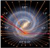 |
Fig. 1 A schematic of the distribution of lines of sight for the GOT C+ Galactic plane survey where they are represented by solid arrows superimposed on an artist’s impression of the Galaxy (R. Hurt, Courtesy NASA/JPL-Caltech). Each arrow represents many lines of sight as they are too dense to display. The longitudinal spacings are indicated on the figure and regions of different angular spacing are separated by dashed arrows. The finest spacing is 0.87° towards the innermost Galaxy and increases outwards. The red lines mark the range l = 270° to 57° of data analyzed in this paper. The area covered from l = 90° to 270°, which is mostly in the outer Galaxy, is only about 20% to 25% of the area of the disk and consequently a larger angular spacing is used, varying from 4.5° at 90° and 270° to 12° near 180°. |
We also observed out of the plane at b = ± 0.5° and ±1°, alternating above and below the plane at each successive longitude. Thus we have half as many positions surveyed at each value of b out of plane as at b = 0°, corresponding to a total of ~450 lines of sight in the disk. Details of the observational mode of [C ii] are given in Paper I along with a discussion of the data reduction. We also observed the J = 1 → 0 transitions of 12CO, 13CO, and C18O with the ATNF Mopra 22-m Telescope (details in Paper I), with an angular resolution of 33′′ toward each line of sight in the inner Galaxy over a longitude range l = 270° to 57°. We obtained H i data from public sources (McClure-Griffiths et al. 2005; Stil et al. 2006). Table 1 is a list of the facilities used, angular resolution, and reference to the data source.
Observational facilities.
We will be using these tracers to derive column densities of H i, CO, and [C ii] in individual line of sight components. However the spatial resolution of the [C ii] observations is the smallest of the tracers. Comparison of the column densities can be problematic if the H i and CO emissions are inhomogenous on scale sizes much smaller than their angular resolution. Higher resolution studies of CO show inhomogenieties down to the resolution limit (cf. Falgarone et al. 2009, and references therein). The area of the CO beam is about 7.6 times that of [C ii] and the H i beam is 25 to 100 times larger than that of [C ii]. There is no precise way for us to estimate the filling factors in the absence of higher resolution CO and H i data. However recent VLA maps of H i in a small slice of the Galactic plane from the THOR (The HI/OH/Recombination line) survey do not show significant inhomogeneity on 20′′ scales (S. Bihr, priv. comm.). Furthermore, if the majority of our H i data were significantly beam diluted then they would scale up to intensities and column densities that exceed those generally found in Galactic surveys (cf. Dickey & Lockman 1990).
We will primarily be using 12CO to calculate column densities of the molecular gas, as this tracer is more uniform than 13CO and spatially more widespread. Towards a few GOT C+ lines of sight there are on-the-fly cuts that show that the [C ii] emission is extended over the angular size of the H i and CO beams (T. Velusamy, priv. comm.). As GOT C+ is the first large scale spectrally resolved Galactic survey of [C ii] and the auxiliary data are the best available for each line of sight, it is not unreasonable to assume that the emission is uniform over the respective beams. We can compare beam averaged intensities because we do not use them to discuss the properties of any individual clouds but instead focus on a statistical analysis of a large number of sources.
In this paper we focus on the inner Galactic plane survey where we have a complete set of H i and high angular resolution CO, consisting of 320 lines of sight covering l = 270° to 57° as indicated with red lines in Fig. 1 and b = 0°, ± 0.5°, and ± 1.0°. Note that the area used in this paper from 270° to 57° (marked in red lines) is about 65% of the entire disk area and so gives a substantial sampling of [C ii] sources in the disk especially as there are fewer detectable sources in the outer Galaxy (see Paper I). Examples of our data are shown in Fig. 2 for three lines of sight where we plot the main beam temperature of the [C ii], H i, and CO isotopologues, along with the Gaussian fits to the [C ii] spectra (see Sect. 3). In many lines of sight the [C ii] features are clearly blends of several components and it can be seen that a wide variety of clouds are detected in [C ii] some with and some without 12CO, as well as many clouds also seen in 13CO, and even C18O; there are also a number clouds detected in 12CO but not [C ii].
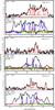 |
Fig. 2 Spectra along three representative lines of sight from the GOT C+ inner Galaxy survey showing Tmb, the main-beam temperature, versus Vlsr. The upper panel for each line of sight shows the [C ii] spectrum along with the fits derived from the Gaussian decomposition (shown in red). The lower panel for each line of sight shows the corresponding H i in black, 12CO in blue, 13CO in red, and C18O in green. The scalings for Tmb are shown in each panel. |
3. Spectral decomposition into [C ii] clouds
In this section we summarize the statistical characteristics of the spectrally resolved components in the inner Galaxy. First we describe the extraction of the cloud components from the spectral line scans, then we discuss the Galactic rotation curve model used to determine their Galactic radius, Rgal. As seen in the sample spectra in Fig. 2 the distribution of [C ii] in velocity is much more limited than that of atomic hydrogen (this difference is also seen in the position-velocity plots in Paper I where the [C ii] spatial-velocity maps are associated with the spiral arms). Carbon is fully ionized in diffuse atomic clouds and these are generally warm enough to excite the C+2P3/2 level. However, the data show that many, if not most, of the H i clouds in the Galaxy have atomic hydrogen densities, n(H), too low to produce emission at the limits of sensitivity of our HIFI survey. Comparing the spectral (and spaxel – see Paper I) distributions of [C ii] and 12CO(1 → 0) we note that there are regions of [C ii] emission without CO, and regions of CO without [C ii]. The former are likely associated with transition molecular clouds and the latter with cold molecular clouds. Finally, the overlap with 13CO is more restrictive, and is consistent with dense molecular clouds occupying a smaller volume of the Galaxy than the diffuse atomic and molecular clouds.
3.1. Spectral decomposition
We identified the cloud components from Gaussian decompositions of [C ii], 12CO, 13CO, and C18O. The [C ii] observations were made with 0.16 km s-1 resolution but to improve the signal-to-noise ratio these data were all smoothed to a velocity resolution of 0.79 km s-1, as were the auxiliary data. In Table 2 we list the velocity resolution used in the analysis and typical 1σ noise per km s-1, in some cases the rms noise for [C ii] was as small as 0.06 K km s-1. We also list the minimum integrated intensity (in units of K km s-1) identified as an emission feature.
The spectra towards most lines of sight are complex with many blended components and their decomposition is very labor intensive. We used an automatic fitting routine but it had to be supplemented with individual inspection of each fit. The spectral lines were fitted with Gaussians using the IDL program XGAUSSFIT developed for use with FUSE data by Lindler (2001). We modified the program to allow up to 30 Gaussians to be fitted over the total bandwidth. XGAUSSFIT is an interactive, least-squares, multiple Gaussian fitting routine. It automatically fits the main component, while additional components must be added by hand, by specifying an initial guess for the central velocity, peak antenna temperature, and Gaussian linewidth of the component. The program then refines the fit for all of the components simultaneously. Further details for how the routine works can be found in Lindler (2001).
Observational sensitivity.
For each line of sight we started by fitting Gaussians to the C18O data as these spectra are better isolated from one another due to their relative scarcity and low opacity (see the examples in Fig. 2). To facilitate the fitting procedure each spectral band was inspected by eye and initial guesses made for the velocity, peak, and width of the line where they could be clearly identified and then XGAUSSFIT determined the best fit. The central velocities and linewidths of the refined Gaussians were then used as the starting point for the fits to the 13CO spectra and then XGAUSSFIT was used to fit the remaining 13CO features, and so on, working through 12CO and finally the [C ii] spectra. At each stage additional initial inputs were provided from inspection by eye where there was no corresponding component from the previously analyzed species. In this way we built up the spectral decomposition working from the least complex spectral tracer to the most complex ones, 12CO and [C ii]. At each stage the fitting program was allowed to add additional Gaussians if necessary to fit the data. In the fitting procedure adopted here we do not consider that there may be absorption features in the spectral band, in particular for [C ii] and 12CO.
We did not apply a Gaussian fitting procedure to the H i spectra because H i clouds are so widely distributed in the Galaxy that the lines are a blend of many features and it is difficult, if not impossible in most cases, to extract components on a consistent basis. Furthermore, the H i 21-cm emission is mainly sensitive to column density and not local density, so there is relatively less contrast among the H i spectral features. To evaluate the intensity of the atomic component along a line of sight we use the information from the Gaussian fits to [C ii] to determine the velocity range over which to calculate the H i integrated intensity. Figure 2 shows the resulting fits superimposed on the [C ii] spectra along three lines of sight. This procedure yielded over 2200 [C ii] Gaussian components. For each component the Gaussian fit gives main beam temperature, Tmb, peak velocity, Vlsr, FWHM linewidth, ΔV, and integrated intensity, I = ∫Tdv.
We then filtered these components by applying criteria on the intensity and line width. To be a valid component we require that the integrated line intensity signal-to-noise rato be greater than 3. We also constrain our features to have line widths in the range 1.5 to 8.0 km s-1. The channel width of our smoothed data is 0.79 km s-1 and the Gaussian fit needs a few channels, so any fits with FWHM less than ~1 km s-1 are potentially noise spikes. Furthermore, the full width half maximum of thermal H2 is ~1.3 km s-1 at 75 K and of C+ ~0.5 km s-1 , so it is unlikely that the cloud components will have lines much narrower than 0.8 km s-1. To be conservative we set our lower limit for an acceptable component at 1.5 km s-1. Although the majority of the [C ii] lines are well fit by a narrow Gaussian, the XGAUSSFIT procedure generates a number of very broad weak lines that represent the residual after the narrower lines are removed from the total spectrum. About 1% of the total number of lines have features with ΔV > 20 km s-1 and about 8% have ΔV that lie in the range 10–20 km s-1. Almost all of these broad weak features are unlikely to be individual clouds, but could be emission from the WIM or WNM (cf. Velusamy et al. 2012), the blending of many low column density, low density CNM features, or artifacts of the fitting procedure. In this paper we take a conservative approach and exclude these broad components from our analysis and set an upper limit of 8 km s-1 . We are left with 1804 narrow [C ii] lines with 1.5 km s-1 ≤ ΔV ≤ 8 km s-1 inside a Galactic radius Rgal ≤ 9 kpc. The 1804 [C ii] components have a mean ΔV = 3.4 km s-1 and about ~80% lie in the range 1.5 to 6.0 km s-1.
3.2. Spatial location in the Milky Way
For each Gaussian component we use the fitted Vlsr along with a Galactic rotation curve model to locate the source of the emission as a function of Galactic radius. We use a smooth model fit to tangent point velocities inside the solar radius (R⊙ = 8.5 kpc), with a flat rotation curve (V⊙ = 220 km s-1) beyond the solar radius (cf. Johanson & Kerton 2009; Levine et al. 2008). For sources near l = 0° it is difficult to assign distances with a smooth rotation curve alone. For these sources we adopt a rotation curve based on the hydrodynamical models of Pohl et al. (2008) following the procedure used by Johanson & Kerton (2009) and using the code given to us by C. Kerton (priv. comm.). Pohl et al. (2008) use a gas-flow model derived from smoothed particle hydrodynamics (SPH) simulations in gravitational potentials based on the near-infrared (NIR) luminosity distribution of the bulge and disk (Bissantz et al. 2003). This approach provides a more accurate kinematics of the clouds in the inner Galaxy especially in the range −6° ≤ l ≤ +6°. This model allows us to use all the observed velocity components including those which are not consistent with realistic solutions from a simple rotation curve. Over most of the range of l within the solar circle discussed here, for a given Vlsr and l, the rotation curves yield near and far distances and a unique value for the Galactic radial distance. We do not attempt to resolve the near-far distance ambiguity as we are interested only in the radial distance from the Galactic center.
In Fig. 3 we plot the radial distribution of [C ii] sources for | b | = 0°, 0.5°, and 1°. The majority of the sources are located between 4 and 7.5 kpc and the median values are 5.8, 5.7, and 6.0 kpc for | b | = 0°, 0.5°, and 1°, respectively. For all sources combined the median radius is 5.8 kpc. The distributions are affected by two factors, the angular sampling and the value of b. As mentioned in Sect. 2, for sources with b ≠ 0° the line of sight samples the volume near the solar system better than further away, such that more [C ii] and CO sources will be intercepted closer to the solar system. This unavoidable factor will skew the radial distribution to Galactic radii closer to the solar system, and is responsible for some of the shift in the distribution. The distributions for | b | = 0.5° and 1° are slightly narrower in Galactic radius than that for b = 0° and there is a slight skewing of the data for | b | = 1° with relatively fewer sources inwards of 4 kpc. This shift for b ≠ 0° is due to the line of sight being at a distance away from the plane greater than the thickness of the Galactic disk at some distance from the solar system and thus not uniformly sampling clouds across the Galaxy. The thickness of the [C ii] gas in the Milky Way is estimated to be of order 150 pc (Paper I) so that near l = 0° sources inward of Rgal = 4 kpc at b = ± 1° are ~80 pc above or below the plane. This undersampling at | b | ≥ 0.5° is reflected in the decrease in the distribution of clouds seen in Fig. 3.
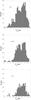 |
Fig. 3 Number distribution of [C ii] sources as a function of Galactic radius for b = 0°, ± 0.5° combined, and ± 1° combined. With increasing b there are fewer sources and their distribution skews closer to the solar radius because the line of sight at some distance away from the solar system is above the plane where there a fewer sources; see text for details. |
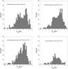 |
Fig. 4 Distribution of [C ii] sources as a function of Galactic radius for clouds as characterized by the presence or absence of CO isotopologues. All values of Galactic latitude, b, are included in this figure. |
3.3. Distribution of clouds by gas tracers
We have catalogued all the [C ii] clouds and labeled them according to the presence or absence of 12CO and 13CO, which depends on the sensitivity of our survey to these isotopologues. We require that all CO spectra have an integrated intensity with a signal-to-noise greater than 3. The typical rms noise and minimum detected intensity for 12CO, 13CO, and C18O in our data base of 1804 clouds are given in Table 2. The corresponding threshold column densities needed to detect these CO isotopologues was estimated using the approximate formulas in Carpenter (2000) assuming optically thin thermalized lines (these were also checked against the RADEX code van der Tak et al. 2007 using typical densities (n(H2) ~ 300 to 1000 cm-3) and temperatures (10 to 40 K)). The resulting minimum column densities are N(12CO) ~ 1–2 × 1015 cm-2, and for N(13CO) and N(C18O) ~ 4–8 × 1014 cm-2. The majority of the CO isotopologue lines are much stronger than these threshold values. In Appendix A.4 we discuss some properties of the relationship among the 12CO and 13CO isotopologue intensities.
Clouds with no detectable CO are labeled diffuse molecular (H2) clouds (as was shown in Langer et al. 2010 and Velusamy et al. 2010, very few [C ii] sources are diffuse atomic H i clouds), while those with 12CO, but no 13CO are transition molecular clouds, and the clouds with 13CO are referred to as dense molecular clouds because they have higher column and, likely, volume densities (those with C18O may be even more highly evolved with denser interiors and cores). In Table 3 we summarize the number of lines of sight and number of clouds by their classification. For all the narrow line [C ii] and CO isotopologue data we created a data base of longitude, latitude, Vlsr, FWHM, integrated intensities, and Galactic radius, Rgal. As discussed above the 21-cm H i spectra are so strongly blended that it is not, in most cases, possible to extract them individually using the Gaussian fitting technique adopted for [C ii] and CO. Later on we will need to know the column density of atomic hydrogen towards each [C ii] source. For the atomic hydrogen tracer we calculate the H i intensity in each cloud by integrating within the velocity widths defined by the [C ii] and/or CO lines.
Number of [C ii] clouds by type and Galactic latitude.
In Fig. 4 we plot the number distribution of [C ii] clouds by category labeled diffuse molecular, transition molecular, and dense molecular cloud, as a function of Galactic radius; in the case of the dense molecular clouds we further separate them by the presence or absence of C18O. The distributions of the different cloud categories are generally similar. They are mostly confined to R = 4 to 7.5 kpc, although the diffuse clouds (no CO) are more extended beyond 7.5 kpc, while the densest clouds, those containing C18O are more confined to 4.5 to 6.5 kpc. As discussed for Fig. 3, the line of sight sampling can skew the distribution to enhance the number of sources closer to the solar system and therefore at larger Galactic radii within the solar circle.
In addition to these sources, we have 714 clouds detected in 12CO in the inner Galaxy without any corresponding [C ii] (at the 4σ level). Their distribution by latitude is given in Table 3 and displayed by Galactic radius in Fig. 5. In contrast to the CO sources with [C ii], the distribution of CO sources without [C ii] is skewed towards larger Galactic radii 7 to 9 kpc. Two factors contributing to this distribution, similar to that seen in [C ii], is that for b = ± 0.5° and ± 1°, clouds above the plane and inside of Rgal about 4 kpc would be missed along these lines of sight and the volume near the solar system is better sampled.
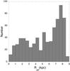 |
Fig. 5 Distribution of CO sources without detectable [C ii] as a function of Galactic radius; all values of Galactic latitude, b, are included in this figure. |
4. CO-dark H2 in clouds
In Langer et al. (2010) and Velusamy et al. (2010) we showed, based on a limited cloud sample, that the observed emission of [C ii] could not be explained by diffuse atomic clouds, and that it requires a significant fraction of [C ii] coming from FUV illuminated molecular gas – the CO-dark H2. In Velusamy et al. (2013) we confirmed this result based on preliminary extraction of a larger data set from the complete survey. Using the complete GOT C+ data set (Paper I) we calculated the azimuthally averaged radial distribution of ISM gas components including the CO-dark H2. Here we expand on these earlier studies and analyze the column densities of different gas components, as traced by H i, [C ii], and CO, on a cloud-by-cloud basis using our sample of 1804 [C ii] clouds. First we re-examine the relationship of [C ii] and H i for these clouds showing that the observed [C ii] cannot arise solely from diffuse atomic gas for the vast majority of the clouds.
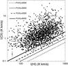 |
Fig. 6 Scatter plot of I([C ii]) versus I(H i) for all [C ii] sources. The straight lines are predicted I([C ii]) for low density atomic H i diffuse clouds as a function of I(H i) (which is proportional to the H i column density) for four different characteristic pressures from P = 2000 K cm-3 to 6000 K cm-3. This pressure range covers predicted values for the diffuse clouds from Rgal ~ 10 kpc to ~4 kpc, with 3000 K cm-3 characteristic of the solar radius. It is clear that the vast majority of the GOT C+ [C ii] sources require an additional source of [C ii] emission other than the diffuse atomic gas. The 1-σ noise for I([C ii]) is indicated on three representative low intensity points; those for I(H i) are too small to be visible on this figure and have been omitted. It can be seen on the scale of this figure that the S/N is high for most of points in this scatter plot. |
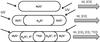 |
Fig. 7 Schematic of the [C ii] emission from different types of clouds along the line of sight. |
In Fig. 6 we plot on a log-log scale the integrated intensity I([C ii]) = ∫T([C ii])dv, versus that for H i, I(H i) = ∫T(H i)dv for all sources. We note several characteristics of this scatter plot. First, I([C ii]) is detected even for very small values of I(H i) ≤ 100 K km s-1, corresponding to a low column density of diffuse atomic hydrogen N(H i) ≤ 1.8 × 1020 cm-2. Second, the largest values of I(H i) yield a column density, N(H i) ~ 2 × 1021 cm-2, or about AV = 2 mag. The column density for typical H i diffuse clouds is less than a few ×1020 cm-2 and for the atomic envelopes of molecular clouds it ranges from ~1 to 7 ×1020 cm-2 (see Fig. 7 in Wolfire et al. 2010). Thus this emission probably arises from several such clouds and/or the H i envelopes around dense molecular clouds in proximity along the line of sight. Third, for any given value of I(H i) there is a large scatter in I([C ii]) indicating that the [C ii] is probing a wide range of cloud conditions and column densities.
We cannot rule out that some of the scatter could be due to the different beam sizes used to observe [C ii] and H i, because, as the beam sizes are very different, there may be detections where we underestimate the H i intensity if the emission is very nonuniform. However, we do not believe that beam dilution is a large factor in Fig. 6 for two reasons. First, as discussed in Sect. 2, VLA 21-cm observations from the THOR survey do not show significant variations on a 20′′ scale. Second, the highest H i intensities in our map ~103 K km s-1 (corresponding to a column density ~2 × 1021 cm-2; see Appendix A.1) and, if the filling factor correction were large, it would shift many points outside the range of intensities found in Galactic H i surveys (cf. Dickey & Lockman 1990). Furthermore, in a few locations there are on-the-fly [C ii] maps that show that the [C ii] emission is extended over the angular size of the H i beam (T. Velusamy, priv. comm.). Finally, our analysis is statistical in nature and some N(H i) may be underestimated while others are overestimated, but on average should represent the characteristics of the H i to [C ii] ratio. Therefore we assume we can use the beam average values of I(H i) and I([C ii]) for this comparison.
We have modeled the expected I([C ii]) as a function of I(H i), similar to what was done in Langer et al. (2010) and Paper I. In those papers we used I(H i) to calculate N(H i), and then we multiplied it by the fractional abundance of C+ with respect to atomic hydrogen, xH(C+), to determine the column density of C+ in the H i gas, NHI(C+). We used a value of xH(C+) = 2.2 × 10⁻⁴ characteristic of the metallicity at of 5.8 kpc, the median Galactic radius for all those sources (see Sects. 3.2 and 4.4 for discussions of the radial distribution and metallicity, respectively). Here we calculate I([C ii]) from the excitation equation (see Appendix A) for a given set of thermal pressures, corresponding to different densities and temperatures, and the same representative metallicity xH(C+) = 2.2 × 10⁻⁴. In Fig. 6 we plot I([C ii]) for a family of (n(H),Tkin) which are labeled with the corresponding pressure, P = nTkin (in units of K cm-3). We fixed the kinetic temperature at a typical value for H i clouds, Tkin = 100 K. For an appropriate range of thermal pressure we were guided by the work of Wolfire et al. (2003). They derived the thermal pressure of low density, low column density atomic clouds based on two-phase thermal pressure equilibrium model of CNM in equilibrium with the WNM, taking into account the variation in metallicity and visible-UV radiation across the Galaxy. As a function of Galactic radius, Rgal in kpc, the pressure is fit by  (1)For Rgal ~ 4.5 kpc to 8.5 kpc, where most sources are located, the pressure lies in the range ~6200 to 3000 K cm-3. We display the predicted I([C ii]) in Fig. 6, for this wide range of typical atomic cloud thermal pressures from P ~ 3000 K cm-3 near the solar radius, R⊙, to ~6000 K cm-3 at the inner radius of the molecular ring. For the GOT C+ sample the median radius of the distribution in Fig. 3 (top panel) is about 5.8 kpc, corresponding to a thermal pressure of ~4900 K cm-3 for H i clouds in the Wolfire et al. (2003) model. The observed I([C ii]) are in general much greater than the values predicted for diffuse atomic clouds. We assume we can use the beam average values of I(H i) and I([C ii]) for this comparison, however as the beam sizes are very different there may be detections where we underestimate the H i intensity on the scale of the [C ii] beam if the emission is very nonuniform. Furthermore, to change our results significantly a large fraction of the samples would have to be significantly beam diluted in H i. We conclude that H i is not a significant collision partner for exciting C+. This conclusion is supported by the fact that [C ii] is not detected over a large (~70%) fraction of the H i emission seen in the wide velocity range over the entire band in all lines of sight, as illustrated in the three examples in Fig. 2. In addition, a spaxel-by-spaxel analysis of the correlation of H i, [C ii], and CO shows that the GOT C+ survey does not detect much [C ii] from low density H i clouds (T. Velusamy, priv. comm.). Thus, the majority of the observed [C ii] in the narrow spectral features comes from FUV illuminated molecular gas, that is the CO-dark H2 gas layer, in clouds. The model for [C ii] emission coming from both H i and H2 gas along the line of sight is discussed in more detail below.
Thus, to determine the properties of the [C ii] clouds we need to calculate the column densities of the three main cloud layers as traced by: H i, [C ii], and CO corresponding to each spectral feature. We assume that most of the H i column density comes from the outermost gas layer in the cloud, but some emission might come from nearby gas along the line of sight within the same velocity range, but not physically associated with the cloud. Such purely atomic H i clouds are likely to be at lower densities than that in the outer layers of denser clouds and their contribution to the total column density can probably be neglected. Below we describe in more detail how we determine the material in each layer. Because we do not map the clouds the results are valid for only one line of sight with the given resolution in each cloud and may not be representative of the cloud as a whole. However, GOT C+ detects so many spectral components that it should represent a statistical sampling of ISM clouds. The assumption adopted here is that the line of sight results represent the properties of the cloud.
4.1. CO-dark H2 model calculation
Figure 7 shows a schematic of what is observed along the line of sight in I([C ii]). This cartoon illustrates three of the line of sight environments sampled by our survey: (top) diffuse atomic hydrogen clouds containing C+ that emit in H i 21-cm and [C ii] 158 μm radiation; (middle) diffuse molecular clouds with atomic and molecular hydrogen layers containing C+ in which there is [C ii] emission from both regions; and, (bottom) transition molecular clouds containing atomic and molecular hydrogen, with unshielded H2 (C+), and shielded H2 (containing 12CO) layers. The transition molecular clouds are traced by 21-cm H i, 158 μm [C ii], and 2.6-mm CO(1 → 0) emission (there is a small neutral carbon layer, or mixed layer containing CO and C+, which does not contain much gas and we omit for simplicity and lack of [C i] data). There are also dense molecular clouds (not shown) which contain, in addition to emission from the 12CO layer in the bottom panel, a deeper layer of 13CO emission and sometimes at larger depths C18O cores.
This schematic and our subsequent analysis ignores the contribution to [C ii] from the WIM for several reasons. First, in Paper 1 we estimated that at b = 0o the WIM contributes on average about 4% to the total intensity of the [C ii] emission. Second, while the relative contribution of the ionized gas can be much larger towards H ii regions or very bright PDRs, the GOT C+ survey intersects very few, if any, of these regions. Third, the filling factor for the WIM and WNM is larger than that for the CNM and thus the WIM and WNM features arise from a longer path length and thus have a broader line width. In Velusamy et al. (2012) we were able to detect directly the [C ii] emission from the WIM, but only along the tangent points in the plane where a relatively small velocity dispersion corresponds to a very long path length, and only at the edge of a spiral arm where the densities are a factor of 2 to 4 higher than in the general interstellar WIM. In other words the intensity per unit velocity is relatively large along the tangent points, whereas towards other lines of sight the emission per unit velocity is much smaller and the WIM (and WNM) does not contribute much [C ii] within the line width characterizing each component in our sample, which are restricted to <8 km s-1. (The WIM is also more important above the plane where its filling factor is much larger, but our narrow line [C ii] components are restricted to ± a few hundred parsecs within the disk.) Thus, as noted in Sect. 3.1, our Gaussian decomposition of [C ii] spectra resulted in residual emission that was very broad but weak, and so removes some of the emission that might arise from the WIM as we only consider the narrow line [C ii] components.
We estimated the fraction of CO-dark H2 gas in our GOT C+ data base using the layered cloud models in Fig. 7. We first determined how much [C ii] emission comes from the H i gas, IHI([C ii]), and then subtract that from the observed total Itot([C ii]) emission. From IH2([C ii]) we can calculate NH2(C+) and then NC+(H2) = NH2(C+)/xH2(C+), where xH2(C+) is the C+ fractional abundance with respect to H2, provided we have an estimate of the densities, temperatures, and fractional carbon abundance in these layers. We determined the contribution of the atomic hydrogen on the line of sight to the total intensity, Itot([C ii]) by calculating N(H i) from I(H i) as described above and in Appendix A. Then we convert it to the corresponding NHI(C+) using the appropriate metallicity for the location in the Galaxy and then determine IHI([C ii]) given the radiative transfer equation in Appendix A, assuming appropriate temperature and density. We set the kinetic temperature to 100 K, characteristic of that measured for H i clouds – the result is not particularly temperature sensitive over the range measured for diffuse clouds. We choose a density from the thermal pressure in the atomic hydrogen gas, n(H i) = P/Tkin, using the pressure gradient in the Galaxy PHI(Rgal) in Eq. (1) above (see also Paper I) derived by Wolfire et al. (2003).
The following list summarizes the steps in our model approach:
-
1.
Use the velocity information and rotation curve to determinethe Galactic radius, Rgal, for each [C ii] and CO source;
-
2.
Determine N(H i) from I(H i) over the velocity range of the [C ii] line;
-
3.
Derive NHI(C+) = xHI(C+)N(H i) using the appropriate Galactic radial value of xHI(C+);
-
4.
Determine the corresponding [C ii] emission intensity, IHI([C ii]), from the H i layer assuming Tkin = 100 K and n(H) = PHI(Rgal)T-1;
-
5.
From the total [C ii] intensity, Itotal([C ii]), subtract the emission coming from the atomic H, yielding the [C ii] emission from the molecular gas, IH2([C ii]) = Itotal([C ii]) – IHI([C ii]);
-
6.
Use IH2([C ii]) to calculate the column density NH2(C+) using the radiative transfer equation in Appendix A, assuming Tkin(H2) and n(H2) from a pressure model of the CO-dark H2 layer (see below);
-
7.
Derive the column density of H2 traced by [C ii], N[CII](H2) = NH2(C+)/xH2(C+);
-
8.
If 12CO is present, then calculate the H2 column density in the CO interior using the CO–to–H2 conversion factor, NCO(H2) = XCOI(12CO).
The details of the relationships and formulas used to calculate the column densities are given in Appendix A. After applying these procedure to all of the [C ii] spectra we have the column densities for each source H i, N(H i), CO-dark H2, N(CO-dark H2) = N[CII](H2), and CO traced H2, N(CO-traced H2) = NCO(H2). The total column density of H2 gas, Ntot(H2) = N(CO-dark H2) + N(CO-traced H2), combines the contribution of the CO-dark H2 and CO-traced H2 layers.
4.2. Density and temperature in the clouds
To calculate the column density NH2(C+) from IH2([C ii]) we need to know the temperature and density of the CO-dark H2 gas (see Appendix A for radiative transfer equations). Unfortunately, C+ has only one fine-structure transition so there is no self-consistent way to determine NH2(C+), n(H2), and Tkin simultaneously. Without information on the density and temperature of the H2 gas we can only determine a combination containing N(C+), n(H2), and Tkin, as can be seen by rewriting Eq. (A.7) in the Appendix as, ![Mathematical equation: \begin{equation} I_{\rm H_{2}}([{\rm CII}]) = 6.9\times10^{-16} N_{\rm H_{2}}({\rm C^+})\frac{n(H_2)}{n_{\rm cr}(H_2)}{\rm e}^{-{\Delta}E/kT}\, (\rm K\, km\, s^{-1}) \end{equation}](/articles/aa/full_html/2014/01/aa22406-13/aa22406-13-eq139.png) (2)where ΔE/k = 91.25 K. We have found that it is possible to combine the dependence on density and temperature and express the column density approximately in terms of just the thermal pressure, P/k = n(H2)T(H2) in units of (K cm-3) times a term that is a weak function of Tkin over the temperature range of interest. Then by specifying the thermal pressure as a function of Galactic radius or with an independent measure of thermal pressure we can estimate the column density of CO-dark H2. If we assume a constant thermal pressure in the [C ii] emitting layer we can replace the density by n(H2) = P(H2)/T where the pressure is in units of K cm-3. As the critical density is a very weak function of kinetic temperature over the temperature range of interest here (Goldsmith et al. 2012) it can be set to a constant and we can rewrite Eq. (2) as,
(2)where ΔE/k = 91.25 K. We have found that it is possible to combine the dependence on density and temperature and express the column density approximately in terms of just the thermal pressure, P/k = n(H2)T(H2) in units of (K cm-3) times a term that is a weak function of Tkin over the temperature range of interest. Then by specifying the thermal pressure as a function of Galactic radius or with an independent measure of thermal pressure we can estimate the column density of CO-dark H2. If we assume a constant thermal pressure in the [C ii] emitting layer we can replace the density by n(H2) = P(H2)/T where the pressure is in units of K cm-3. As the critical density is a very weak function of kinetic temperature over the temperature range of interest here (Goldsmith et al. 2012) it can be set to a constant and we can rewrite Eq. (2) as, ![Mathematical equation: \begin{equation} I_{\rm H_{2}}([{\rm CII}]) = 6.9\times10^{-16} \frac{P({\rm H}_2)N_{{\rm H}_{2}}({\rm C^+})}{n_{\rm cr}({\rm H}_2)}\frac{{\rm e}^{-{\Delta}E/kT}}{T}\cdot \end{equation}](/articles/aa/full_html/2014/01/aa22406-13/aa22406-13-eq144.png) (3)(The term PT-1exp( − ΔE/kT) is related to the collision rate from the lower to the upper state.)
(3)(The term PT-1exp( − ΔE/kT) is related to the collision rate from the lower to the upper state.)
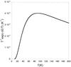 |
Fig. 8 Dependence of T-1exp( − 91.25/T), which is proportional to the relative excitation rate to the |
In Fig. 8 we plot the expression T-1exp( − 91.25/T) as a function of T. It can be seen that it varies by less than about ±15% about its mean value of 3.5 × 10⁻³ over a broad range of temperatures 45 K ≤ Tkin ≤ 200 K and is good to about ±20% down to 40 K). Thus if we have an estimate of the thermal pressure of the H2 layer, the choice of Tkin is not critical over this temperature range. At less than 40 K the excitation rate drops sharply and the choice of Tkin is important. We believe it is unlikely much of the [C ii] emission detected by GOT C+ comes from gas with Tkin < 35 K, although the survey is sensitive to emission down to 20 K depending on pressure and column density. For example, the GOT C+ survey can detect [C ii] in gas down to 45 K for the diffuse molecular clouds (no CO) with column densities at the lower end of their range, N(C+) ~ 1017 cm-2, for typical diffuse gas pressures. For the median column density of these clouds, N(C+) ~ 3 × 1017 cm-2 GOT C+ is sensitive to gas at temperatures down to ~25 K. However, for the dense molecular clouds with high pressure PDRs the GOT C+ survey can detect [C ii] emission down to ~15 K. Thus for warm C+ layers, >40 K, the column density is mainly a function of the thermal pressure in the gas and the column density can be written approximately in the following form using the mean value above for T-1exp( − 91.25/T), ![Mathematical equation: \begin{equation} N_{\rm H_{2}}({\rm C^+})\simeq 4.2\times10^{17} \frac{n_{\rm cr}({\rm H}_2)}{P({\rm H}_2)} I_{{\rm H}_{2}}([{\rm CII}]);\,40~K\! <\! T_{\rm kin}\! <\! 200{\rm K} \end{equation}](/articles/aa/full_html/2014/01/aa22406-13/aa22406-13-eq155.png) (4)where NH2(C+) is in cm-2 and this solution is good to about ±20% over the indicated temperature range. Furthermore, it is reasonable to assume that the thermal pressure is roughly constant across the CO-dark H2 layer, because, as C+ is the primary coolant in the layer, if the density increases the temperature decreases. Thus if we can characterize the thermal pressure as a function of cloud type and Galactic environment, then we can solve for the column density NH2(C+). Note that Eqs. (3) and (4) were derived to demonstrate that use of a constant pressure in the C+ layer is reasonable. However, for all calculations of [C ii] intensity and C+ column density, we use the full radiative transfer equations in Appendix A. Then N(H2) traced by [C ii] is just
(4)where NH2(C+) is in cm-2 and this solution is good to about ±20% over the indicated temperature range. Furthermore, it is reasonable to assume that the thermal pressure is roughly constant across the CO-dark H2 layer, because, as C+ is the primary coolant in the layer, if the density increases the temperature decreases. Thus if we can characterize the thermal pressure as a function of cloud type and Galactic environment, then we can solve for the column density NH2(C+). Note that Eqs. (3) and (4) were derived to demonstrate that use of a constant pressure in the C+ layer is reasonable. However, for all calculations of [C ii] intensity and C+ column density, we use the full radiative transfer equations in Appendix A. Then N(H2) traced by [C ii] is just ![Mathematical equation: \begin{equation} N_{\rm [CII]} ({\rm H_2})= N_{\rm{H_2}}({\rm C^+})/ x_{{\rm H_2}}(\rm C^+) \end{equation}](/articles/aa/full_html/2014/01/aa22406-13/aa22406-13-eq157.png) (5)where xH2(C+) = 2xH(C+), as H2 contains two atoms of hydrogen. Below we discuss an appropriate pressure model for each category of cloud detected in [C ii].
(5)where xH2(C+) = 2xH(C+), as H2 contains two atoms of hydrogen. Below we discuss an appropriate pressure model for each category of cloud detected in [C ii].
4.3. Pressure in the CO-dark H2 gas
To use the approach in Sect. 4.2 to calculate the column density of CO-dark H2 we need to know the thermal pressure in the different types of clouds. For the diffuse low column density molecular clouds (no or very little CO) in the solar neighborhood, the H2 layer containing C+ is observed to have thermal pressures of order a few × 103 K cm-3 (cf. Sheffer et al. 2008; Goldsmith 2013). Densities and temperatures, and therefore thermal pressures, have been determined from observations of absorption lines in the optical and UV for nearby low column density clouds. For example, Sheffer et al. (2008) analyzed UV absorption lines of H2 in diffuse molecular clouds with N(H2) column densities up to ~1021 cm-2 (or AV ~ 1 mag.) and derived Tkin ranging from 50 to 120 K, with an average of 76 K in the molecular portion of the cloud. Goldsmith (2013) derived densities for these clouds from the UV absorption measurements of trace amounts of CO by applying an excitation model wherever reliable measurements existed for two or three of the lowest CO transitions. Goldsmith (2013) finds an average H2 density, ⟨n(H2)⟩ of 74 cm-3 for a kinetic temperature 100 K and 120 cm-3 for 50 K, corresponding to an average thermal pressure in the range 6000 to 7400 K cm-3. Jenkins & Tripp (2001) derived the thermal pressure in diffuse atomic clouds from absorption line measurements of neutral carbon towards 26 stars and find an average pressure of 2240 K cm-3. In a later paper Jenkins & Tripp (2011) extended their analysis to 89 stars and derived a mean pressure of 3800 K cm-3 locally. For the dense molecular clouds, Sanders et al. (1993) estimated that the thermal pressures range from 104 to 105 K cm-3 (see also Wolfire et al. 2010). The pressures in the transition clouds likely lie in between the diffuse and dense clouds.
For the diffuse molecular clouds we adopt the approach taken in Paper I, which uses the Galactic pressure gradient derived by Wolfire et al. (2003) for the diffuse atomic gas, but scaled up by a factor of 1.6 to normalize to a local value intermediate between those of Sheffer et al. (2008); Goldsmith (2013); and Sanders et al. (1993). This yields P(Rgal) = 2.2 × 10⁴exp( − Rgal/5.5) (K cm-3), which has a value of 4700 (K cm-3) at 8.5 kpc. We adopt a characteristic kinetic temperature in the CO-dark H2 layer of 70 K for these clouds. In this paper we will present our results in terms of column density, because the conversion to visual extinction depends on the metallicity which varies across the Galaxy.
The transition molecular clouds (those with 12CO, but no 13CO) have larger column densities, hydrogen densities, and pressures than diffuse molecular clouds. The range of hydrogen column density for these clouds is fairly limited because if they get too thick or dense we should detect 13CO (see for example the models of 12CO and 13CO by Visser et al. 2009). (As we show below for the clouds analyzed here, over 70% of these clouds lie in the range N(H2) = 0.9 to 2.8 ×1021 cm-2, with a median value of 1.7×1021 cm-2 ). For lack of direct measurements of the pressure in these clouds, here we adopt a fixed pressure of 104 K cm-3, at the lower end of the range appropriate for dense 13CO molecular clouds and at the high end of the pressure for the diffuse molecular clouds. In Paper I we assumed a Galactic gradient for the pressure of these clouds, but over the range where most of the sources are detected it represents only a ±20% difference. We adopt a kinetic temperature of 70 K which is consistent with the models of the CO-dark H2 layer in dense molecular clouds by Wolfire et al. (2010).
For the dense molecular clouds with 13CO the assignment of a pressure is far more difficult because the observed range of pressures in Galactic surveys is very large, 104 to 105 K cm-3. These clouds have a narrow shell of C+, the column density of CO can be much larger, up to the upper mass limit of the Giant Molecular Clouds (GMC). Indeed the column density distribution for our sample of 13CO clouds tends to be much broader and flatter than that for the diffuse molecular and transition molecular clouds. Examination of the relationship between the intensities of [C ii] and 13CO provides a clue as to how to evaluate the variation in pressure in these clouds. In Fig. 9 we plot the intensity of [C ii] arising from the H2 gas, IH2([C ii]), derived using Appendix Eq. (A.7) versus I(13CO). Even though there is large scatter in the data there is an overall trend for IH2([C ii]) to increase with increasing I(13CO), especially for larger values of I(13CO), which correspond to the thicker and more massive clouds. A least squares linear fit to the data yields IH2([C ii]) = 1.08 + 0.49 I(13CO) with a correlation coefficient of 0.56, which is statistically a moderately correlated relationship.
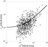 |
Fig. 9 IH2([C ii]), the intensity of [C ii] in the H2 layer plotted against I(13CO) on a log-log scale. There is a trend towards larger IH2([C ii]) with increasing I(13CO). The solid line shows a linear fit to the data, IH2([C ii]) = 1.08 + 0.49 I(13CO), which appears curved when transformed to the log-log plot shown here. The 1-σ noise for IH2([C ii]) is indicated on three points; those for I(13CO) are too small to be visible on this figure and have been omitted. It can be seen on the scale of this figure that the S/N is high for most of points in this scatter plot. |
Chemical models of the abundance profiles of C+ and CO clouds thick enough to produce detectable 13CO yield a roughly constant column density N(C+) whereas N(13CO) can have a very large range of values because C+ comes from the outside layer, whereas the shielded interior where CO is found can be of any thickness within the limits of typical GMC masses and column densities per beam. For example in the models of CO-dark H2 in dense clouds by Wolfire et al. (2010) the thickness of the CO-dark H2 layer varies from N(CO-dark H2) ~ 0.6 to 2.8 × 1021 cm-2, even as the total mass of the cloud increases from 105 to 3 × 10⁶ M⊙ and the strength of the FUV radiation field changes by a factor of 10. Thus we suggest that the large increase in [C ii] emission with increasing 13CO emission is most likely due to an increase in the hydrogen density of the [C ii] emitting layer, and therefore its thermal pressure. Assuming this relationship is correct we can use I(13CO) to estimate the thermal pressure in the [C ii] emitting layer as follows. We use the linear relationship derived for the data in Fig. 9 to scale the thermal pressure used for modeling the dense molecular clouds traced by 13CO. In the limit of vanishing I(13CO) we assume the pressure approaches that of the 12CO transition molecular clouds, assumed above to be ~104 K cm-3, therefore P([C ii]) = 104[1.08 + 0.49I(13CO)] in units of K cm-3. For the [C ii] emitting layer in 13CO clouds we adopt a kinetic temperature of Tkin = 70 K, consistent with the values calculated by Wolfire et al. (2010) which vary from ~50 K to 80 K in the CO-dark H2 transition zone (see their Fig. 4).
4.4. Metallicity
To convert NH2(C+) to N(H2) we need to know the carbon fractional abundance xH2(C+) = n(C+)/n(H2) across the Galaxy. The metallicity fraction per molecular hydrogen is double that in the atomic gas, xH2(C+) = 2xH(C+). Observations in the local interstellar medium lead to xH(C+) = n(C+)/n(H) in the range 1.4 to 1.8 × 10⁻⁴ (Sofia et al. 1997), and here we adopt a value of xH(C+) = 1.4 × 10⁻⁴. However, we need to account for the metallicity gradients in the Galaxy. For the carbon metallicity gradient we adopt the formula discussed by Wolfire et al. (2003) based on the oxygen metallicity gradient derived by Rolleston et al. (2000) over the range 3 kpc <Rgal < 18 kpc, and used in Paper I,  (6)For Rgal < 3 kpc we adopt a constant value, xH(C+) = 3.4 × 10⁻⁴ equal to that at Rgal = 3 kpc. Only a small percentage of our [C ii] sources are at Rgal < 3 kpc and very few ≤ 2 kpc, so any error in setting xH(C+) to a constant in this regime does not affect our results for the mass distributions very much. This value is doubled in the molecular gas and xH2(C+) = n(C+)/n(H2) which yields a local value near the solar system of 2.8 × 10⁻⁴.
4.5. Column densities of the cloud components
To determine the distribution of warm CO-dark H2 gas we calculate the column densities of all the cloud layers (H i, C+, CO) following the procedures outlined in Sect. 4.1 above and in Appendix A for each [C ii] spectral line component. In Fig. 10 we plot a histogram of the column density of the CO-dark H2 layer, N(CO-dark H2) (=N[CII](H2) in Eq. (5)) . For this distribution the median N(CO-dark H2) = 0.7 × 1021 cm-2, the mean value is 1 × 1021 cm-2, and there is a tail extending beyond ~1.4 × 1021 cm-2. About 4% of the sources lie above 2.8 × 1021 cm-2.
About 65% of the sources have a N(CO-dark H2) less than 1 × 1021 cm-2 and ~90% ≤ 1.9 × 1021 cm-2. These values are consistent with cloud-chemical models of low column density clouds (Visser et al. 2009) and the edges of more massive clouds (Wolfire et al. 2010). However, roughly 10% of the clouds in Fig. 10 have larger N(CO-dark H2). Such thick layers of CO-dark H2 are not expected theoretically. It is possible that these large values result from underestimating the true pressure in the H2 gas or arise from several lower column density clouds blended into one broad spectral feature.
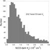 |
Fig. 10 Distribution of the column density of the CO-dark H2 gas layer in all [C ii] sources in the GOT C+ inner Galaxy survey. |
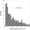 |
Fig. 11 Distribution of column density of the CO-traced gas, N(CO-traced H2) in [C ii] sources. |
In Fig. 11, we plot the distribution of column densities of the CO-traced H2, N(CO-traced H2). There are ~1250 CO sources in this figure, less than the number of C+ sources because a fraction of our [C ii] comes from clouds without CO. The median and mean N(CO-traced H2) are 1.5 and 2.3 × 1021 cm-2, respectively. Over 80% of the clouds have a low CO-traced H2 column density, with N(CO-traced H2) ≤ 3.8 × 1021 cm-2, and ~90% have ≤5.6 × 1021 cm-2. However, unlike the case for the CO-dark H2 layer, there is no restriction on how thick the dense CO-traced H2 interior can be, within the limits of typical GMC masses, and about 3% of the clouds have N(CO-traced H2) > 9 × 1021 cm-2 (not shown in Fig. 11).
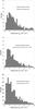 |
Fig. 12 Distribution of the column density of the CO-dark H2 gas layer sorted by type of cloud in the GOT C+ inner Galaxy survey: (top) diffuse molecular clouds; (middle) transition molecular clouds; and, (bottom) dense molecular clouds. |
In Fig. 12 we compare the column density of the CO-dark H2 layers in three types of clouds: diffuse molecular clouds without CO, transition molecular clouds with 12CO but no 13CO, and dense molecular clouds with 13CO (some of which also contain C18O). The distributions of N(CO-dark H2) are similar for all three types of clouds and they have comparable median (0.79, 0.69, and 0.65) × 1021 cm-2 and mean values (1.0, 0.94, and 0.93) × 1021 cm-2. (For reference note that the mean column density for our sample of sources without CO corresponds to AV ~ 1 mag, using the standard conversion to visual extinction in the solar neighborhood.) The mean value of N(CO-dark H2) in the dense molecular clouds is consistent with models of this layer by Wolfire et al. (2010), however, they found a nearly constant thickness of N(CO-dark H2) over a wide range of conditions for the dense clouds, whereas we see significant variability. In the next section we make a more detailed comparison of observations with models.
Figure 13 shows the total H2 column density, Ntot(H2) = N(CO-dark H2) + N(CO-traced H2), for different categories of clouds. The addition of the H i contribution to the column density does not change the distribution much as N(H i) is generally small compared to the other terms in the clouds detected in [C ii]. The peak in the distribution of the total H2 column density in diffuse molecular and transition molecular clouds is narrow, whereas that in the dense molecular clouds is broader. The median total H2 column density is 0.8 × 1021 cm-2 for the diffuse molecular clouds, 1.4 × 1021 cm-2 for the transition clouds, and 3.7 × 1021 cm-2 dense clouds. The breadth of the distribution in the total H2 column density is indicated by the mean values and standard deviation of Ntot(H2), for these three categories: (1.1 ± 0.9) × 1021 cm-2 for diffuse molecular clouds, (1.8 ± 1.3) × 1021 cm-2 for the transition molecular clouds, and (4.4 ± 2.9) × 1021 cm-2 for the dense molecular clouds. The distribution for all the [C ii] sources combined is given in the lower-right panel of Fig. 13. This distribution has a median Ntot(H2) = 1.8 × 1021 cm-2, and a mean value of (2.6 ± 2.5) × 1021 cm-2. Overall, about 80% of the sources have a total molecular hydrogen column density less than 4 × 1021 cm-2 and ~90% have total H2 column densities ≤5 × 1021 cm-2. Fewer than 2% of the sources have large column densities, ≥10 × 1021 cm-2, most of which are detected in C18O; these could be dense PDRs. About 30% of the sources have a low total H2 column density ≤1 × 1021 cm-2.
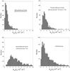 |
Fig. 13 Distribution of total H2 column density for different types of clouds: (top left) diffuse molecular clouds with no CO; (top right) 12CO transition molecular clouds; (bottom left) dense molecular clouds with 13CO; and (bottom right) all [C ii] sources. Note that the vertical scale is different in the last panel. |
4.6. CO-dark H2 mass distribution
We use the column densities to calculate the fractional mass, f, in the CO-dark H2 gas in each cloud using, 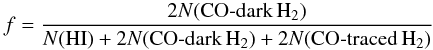 (7)where the factors of two account for the mass of H2 compared to atomic hydrogen. Unlike the analysis in Paper I, which derived the fraction of CO-dark H2 gas in the Galactic ISM, here we calculate only the fractional mass of CO-dark H2 in each cloud and how the distribution of f might differ among the various categories of clouds. In Fig. 14 we plot the distribution of f for: diffuse molecular hydrogen (no CO), transition molecular clouds, and dense molecular clouds with 13CO but no C18O, and dense molecular clouds with C18O). As expected the diffuse molecular clouds have the largest fraction of CO-dark H2 by mass because they do not have extensive molecular cores. In contrast, the dense molecular clouds, as traced by 13CO, have significant molecular gas in their shielded cores and their CO-dark H2 mass fraction is much smaller. The dense C18O clouds tend to have the largest CO column densities and so the smallest fraction of CO-dark H2. The 12CO transition molecular clouds lie somewhere in between and have a very broad range of f.
In Fig. 15 we plot the distribution of fractional mass in the CO-dark H2 gas layer for all the [C ii] clouds. The two peaks correspond to diffuse molecular and dense molecular clouds. In Table 4 we list the median of the fractional mass of CO-dark H2 gas, its mean value ⟨f⟩, and 1σ standard deviation.
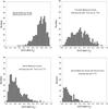 |
Fig. 14 Fraction by mass of CO-dark H2 gas for different classes of clouds: (upper left) diffuse molecular clouds, the [C ii] sources with no CO; (upper right) transition molecular clouds, [C ii] sources with only 12CO; (lower left) dense molecular clouds, with 13CO and no C18O; and, (lower right) dense molecular clouds with 13CO and a dense C18O core (or cores). |
Mass fraction of CO-dark gas.
The diffuse molecular clouds detected in the GOT C+ survey have significant fractions of CO-dark H2 gas, typically more than 70 per cent. The fact that so few purely atomic H i diffuse clouds are present in the data set (i.e. those with little or no H2) is due to a lack of sensitivity to [C ii] for low H i column and/or low volume density clouds. For the transition molecular clouds the distribution in f(CO-dark H2) is shifted towards lower values and ⟨f⟩ ~ 0.4. This result is consistent with our picture of the profile of carbon in clouds: it is primarily ionized in the envelope and makes a somewhat sharp transition to CO (with a narrow layer mixing C+, C, and CO) as the FUV radiation is attenuated by dust, H2 lines, and CO line self-shielding. In the dense molecular clouds where 13CO is detected, the CO molecular gas region is even thicker and the fraction of CO-dark H2 becomes smaller, with ⟨f⟩ ~ 0.2. Taken together the ensemble of [C ii] clouds have a mass fraction of CO-dark H2, ⟨f⟩ ~ 0.44. These results omit the contribution of CO clouds where we do not detect [C ii]. In Paper I the contributions of all the [C ii] and CO gas is taken into account in deriving a Galactic radial solution to the fraction of CO-dark H2, and yields a smaller fraction, ⟨f⟩ ~ 30% averaged over the entire Galaxy.
5. Comparison to cloud chemical models
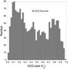 |
Fig. 15 Fraction by mass of CO-dark H2 gas for all the [C ii] sources. |
Over the past forty years ever more sophisticated models have been constructed of PDRs taking into account the many physical and chemical processes that determine their structure. In interstellar clouds photodissociation of CO by UV is the most important destruction mechanism and photoionization keeps carbon ionized. Hence the treatment of the photodestruction processes and the corresponding radiative transport in the cloud is key to modeling the C+ to CO transition and calculating the thickness of the CO-dark H2 layer. Here we compare our results to the recent cloud chemical models of the transition from C+ to CO by Visser et al. (2009) and Wolfire et al. (2010). The depth of the transition from C+ to CO yields the column density of the CO-dark H2 layer.
The models of Visser et al. (2009) were aimed at understanding the depth dependence of the onset of the formation of CO and its isotopologues under a variety of cloud conditions. They used a semi-infinite slab model and integrate step-wise into the clouds to calculate the UV radiation field. Attenuation of the radiation includes continuum absorption by dust, shielding by H2 and CO, and self-shielding of CO isotopologues using the latest laboratory and theoretical values for the line parameters. They adopted the benchmark chemical network and chemical reaction rates from a PDR benchmark study (Röllig et al. 2007). This reaction network incorporates 31 atomic and molecular species consisting only of H, He, C, O, and electrons, however they add the 13C, 17O, and 18O isotopes and the corresponding isotope exchange reactions. The addition of isotopes of carbon and oxygen increases the number of species to 118 and the chemical reaction network to 1723. The restriction to 118 species focus on the key carbon network producing CO, while keeping the number of reactions manageable for a parameter study. (Note, some very large networks and data bases contain over 400 species and over 4500 reactions (cf. McElroy et al. 2013) without isotopes, so any full network chemistry including isotopologues would be much more computationally demanding for modeling the cloud chemistry over a large parameter space.) The restricted network does leave out potentially important species for the ionization balance, such as sulfur (cf. Röllig et al. 2007, Sect. 3.1.2).
Visser et al. (2009) calculate the abundances and column densities of the CO isotopologues in diffuse and transition molecular clouds (Av ≤ 4 mag.) for a range of physical parameters. They calculated N(CO) as a function of N(H2) for a grid covering the following range of parameters: n(H2) = 100–1000 cm-3, Tgas = 15–100 K, and FUV strength χ = (1–10)χ0, where χ0 is the local value in the solar neighborhood, for about 60 model runs. They plotted the results for all the depth steps in their grid for all the parameters n(H2), Tgas, and χ. The output consists of thousands of model values for the column density of the CO isotopologues as a function of N(H2). Details of their model results are presented in figures and tables both in their text and on-line. Figure 7 in Visser et al. (2009) displays N(12CO) versus N(H2) for all points with AV < 4 mag. from their grid of cloud models. The scatter in the model results is due to the different physical parameters assumed for the cloud models. In addition to the set of maximum and minimum column densities of N(CO), they also generate a 100-point mean of the model results by averaging the solutions in fixed grid regions at over 30 depths into the cloud to facilitate comparison to observations. They found that the transition from a C+ to a CO dominated regime can occur over a wide range of N(H2) from ~a few × 1020 to ~2 × 1021 cm-2 (see their Fig. 7).
Wolfire et al. (2010) modeled the thickness of the CO-dark H2 layer in a spherical model of massive dense molecular clouds and considered the effects of the strength of the FUV field, metallicity, density, and cloud mass. They found that for χ in the range (3–30)χo the CO-dark H2 column density, which they measured in AV, varies very little. However, they did find that the solutions depended on the metallicity (see their Fig. 10).
In Fig. 16 we plot N(CO-dark H2) as a function of the total hydrogen column density, Ntot = N(H i) + 2N(H2), for all clouds detected in CO in our survey up to Ntot = 1022 cm-2. For comparison we have plotted some of the results from Visser et al. (2009) in Fig. 16. We have used the solutions for N(CO) versus N(H2) in their Fig. 7 and the Tables to calculate the upper and lower bounds on N(CO-dark H2) and for their 100–point mean solution. To calculate N(CO-dark H2) from Visser et al. (2009) we first calculate the total carbon column density, Ntot(C) = xH(C)Ntot, and then N(C+) = Ntot(C) – N(CO), and finally N(CO-dark H2) = N(C+)/ xH2(C+), where we neglect the small contribution from N(H i).
From these column densities we calculate the boundary of the maximum, minimum, and 100-point mean fraction N(CO-dark H2) and plot them in Fig. 16. While many data points fall within the bounds of their models, the majority of the clouds have much less N(CO-dark H2) than the models. However, in comparing our values of N(CO-dark H2) to the model values it must be kept in mind that Visser et al. (2009) assume a metallicity appropriate to the solar neighborhood which does not apply to most of the sources in our survey. In the work of Wolfire et al. (2010) on much more massive clouds they found that an increase in metallicity resulted in a lower column density of CO-dark H2 all other factors kept equal. There is no comparable set of models with different metallicity along the lines of Visser et al. (2009) available for more detailed comparison.
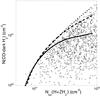 |
Fig. 16 Column density of CO-dark H2 gas for all CO sources as a function of the total hydrogen column density Ntot = N(H i) + 2N(H2). The curves are N(CO-dark H2) calculated from the models of Visser et al. (2009) as discussed in the text. The central curve (dashed line) is the 100-point means of their model shown in the right panel of their Fig. 7. The top curve (dotted line) is the lower limit on the solutions for N(CO), which yields a maximum for N(CO-dark H2), and the bottom curve (solid line) is the upper limit on N(CO), which yields a minimum for N(CO-dark H2), as a function of N(H2) for the range of parameter space used in their models. |
In Fig. 17 we plot f(CO-dark H2) as a function of the total hydrogen column density, Ntot = N(H i) + 2N(H2), for all 1804 sources, separated into the three cloud categories: diffuse molecular (red °), 12CO transition clouds (blue ×), and the dense 13CO clouds (black △). The sources cluster in regions as expected with the diffuse clouds having the highest f(CO-dark H2) on average and the dense clouds the lowest values, corresponding to the distributions seen in Fig. 14. For comparison we again use the results from Visser et al. (2009) and include those from Wolfire et al. (2010) in Fig. 17. The figure shows just how large and variable are the model f(CO-dark H2). As can be seen only about half the GOT C+ sources fall within the maximum and minimum curves from Visser et al. (2009), but this result is not unexpected as at higher metallicity N(CO-dark H2) will be lower for a given Ntot, as discussed for Fig. 16. For example at Rgal ~ 4 kpc the metallicity is double the solar value, and curves for f(CO-dark H2) will be approximately proportionally lower. Furthermore the Visser et al. (2009) models are limited to a visual extinction ~4 mag. so do not model massive clouds with large column densities. In contrast Wolfire et al. (2010) only model very massive clouds with high average column densities corresponding to N(H2) = 7.5 and 15 × 1021 cm-2, but they do consider the dependence of f(CO-dark H2) on metallicity, where Z′ = Z/Z⊙ is the metallicity with respect to the solar value.
In Fig. 17 we also plot the solutions for f(CO-dark H2) from Wolfire et al. (2010) for three values of the metallicity with respect to the solar value, Z′ = 0.5 (red), 1.0 (blue), and 1.9 (black) times Z⊙, where Z⊙ is the solar value. These values correspond to Galactic radii, Rgal = 12.8, 8.5, and 4.5 kpc, respectively. For each value of Z′ there are two model points corresponding to Ntot = 1.5 × 10²² and 3 × 1022 cm-2 (or N(H2) = 7.5 and 15 × 1021 cm-2 in Wolfire et al. 2010). We connect these points with a linear fit in Fig. 17. For the enhanced metallicity, f(CO-dark H2) is lower, ranging from 0.25 to 0.17. Here again our values for f(CO-dark H2) are generally smaller than that modeled by Wolfire et al. (2010) for the massive clouds with large column densities. However, the median value of f(CO-dark H2) for the GOT C+ data base of dense 13CO clouds is 0.18 (Table 4) in rough agreement with the values from Wolfire et al. (2010).
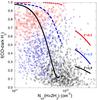 |
Fig. 17 Fraction by mass of CO-dark H2 gas for all sources as a function of the total hydrogen column density Ntot = N(H i) + 2N(H2): diffuse molecular clouds (red °), 12CO transition molecular clouds (blue ×), and 13CO dense molecular clouds (black △). The curves on the left are f(CO-dark H2) calculated from the models of Visser et al. (2009) as discussed in the text. The central curve (dashed blue line) is the 100-point means of their model shown in the right panel of their Fig. 7. The top curve (dotted red line) is the lower limit on the solutions for N(CO), while the bottom curve (solid black line) is the upper limit on N(CO) as a function of N(H2) for the range of parameter space used in their models. On the right side we plot the few values of f(CO-dark H2) calculated by Wolfire et al. (2010) for massive clouds for different values of metallicity relative to the solar value, Z′ = 0.5 (red line), 1.0 (blue line), and 1.9 (black line). |
As seen above, lower metallicity results in clouds with larger f(CO-dark H2) so we expect that there should be a Galactic gradient in f(CO-dark H2). In Paper I we found that the azimuthally averaged fraction of CO-dark H2 increases with Galactocentric distance, and we get a similar trend using the cloud components. We divided the Galaxy in 0.5 kpc rings and summed all the H i, CO-traced H2 and CO-dark H2 column densities within each ring from sources with [C ii]. Including the CO sources without [C ii] introduces an uncertainty in how much hidden CO-dark H2 there is in these clouds. We used these values to calculate the average f(CO-dark H2) within each 0.5 kpc thick ring and plot the results in Fig. 18. We see a systematic trend for f from about 0.2 in the inner Galaxy to ~0.55 at R⊙. This trend is consistent with the results expected for a metallicity gradient and because there are relatively more diffuse molecular clouds, with higher f(CO-dark H2) values, approaching R⊙ and relatively more massive clouds, as indicated by the C18O clouds in the interior (see lower right panel in Fig. 4, with much smaller f(CO-dark H2). While the exact values of f(CO-dark H2) in this figure may be slightly uncertain because we cannot calculate the corresponding CO-dark H2 for the clouds seen in CO but not [C ii], we expect the overall trend to be valid.
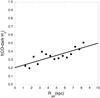 |
Fig. 18 Distribution of f(CO-dark H2) in CO sources with detectable [C ii] averaged over rings as a function of Galactic radius. |
6. Summary
The GOT C+ survey is the first step in providing a velocity resolved map of the [C ii] in the Galactic disk. In Paper I we discussed the global distribution of H i, CO, and [C ii] and derived the azimuthally averaged distribution of ISM gas components for b = 0°. In this paper we have used the spectral information to extract individual cloud features in [C ii] and characterized statistically the properties of clouds as labeled by whether they also contained 12CO and 13CO. The approaches used in Paper I and the present work complement each other. While Paper I accounts for all the [C ii] intensity detected in the survey, the present work accounts for only about 50%, the fraction of the [C ii] intensity identified in narrow line (ΔV ≤ 8 km s-1) clouds. Thus here we provide a better picture of the global cloud properties while Paper I provides a better picture of the Galactic global [C ii] distribution of each ISM component.
We identified over 1800 narrow line [C ii] features in the inner Galaxy bounded by l = 270° to 57°, b ≤ ± 1°, and Rgal ≤ 9 kpc. These [C ii] features were subdivided into three categories of clouds depending on the presence of CO isotopologues as follows: 557 diffuse molecular clouds with no CO; 513 transition molecular clouds with 12CO, but no 13CO; and, 734 dense molecular clouds with 13CO (212 of these dense clouds also had C18O). In addition, we identified 714 CO emitting clouds with no detectable [C ii] at the level of the sensitivity of the GOT C+ survey. Thus it appears that our [C ii] survey is sampling a good distribution of clouds at different evolutionary stages across much of the Galactic disk. The distribution of clouds in all [C ii] categories is roughly flat between 4 and 7 kpc, but the CO clouds without [C ii] have a peak around 8 kpc.
We used our [C ii] data base along with CO isotopologue and H i observations to calculate the gas column density of different layers of the cloud: diffuse H i envelope, warm CO-dark H2 envelope, and CO interior. In the case of [C ii] there is only one transition to work with and so, to estimate the density and temperature in the [C ii] emitting layer, we have adopted a constant temperature in the layer and use thermal pressure models to determine the likely hydrogen density. The thermal pressure of the layer varies in a systematic way (on average) as one progresses from low density diffuse molecular clouds to the dense molecular clouds. We find that the mean column density of CO-dark H2 is similar for the three types of clouds with Ntot = 1.0 × 1021 cm-2, 0.94 × 1021 cm-2, and 0.93 × 1021 cm-2 as one progresses from diffuse molecular, through CO transition molecular, to dense 13CO molecular clouds.
We calculated the fractional CO-dark H2 mass in each cloud and find that it decreases from an average of ~77% in the diffuse molecular clouds, with no CO interiors, to as little as ~20% in the dense molecular clouds with 13CO cores. The fraction in diffuse and transition molecular clouds is in general less than that calculated in the Visser et al. (2009) models, but this might be due to the choice of metallicity adopted in their models which is lower than that where most of our sources are located in the Galaxy. The fraction in the dense molecular clouds is ~21% compared to the roughly 30% predicted in the dense cloud models of Wolfire et al. (2010). While the mean column densities and f(CO-dark H2) are roughly in agreement with the models of Wolfire et al. (2010), we find more dispersion in the actual data than predicted by their models. This dispersion could be due to the application of our thermal pressure model to an ensemble of clouds, rather than knowing the exact pressure for each cloud, or it could be real, but it will take additional probes of the pressure to decide. We conclude that a significant fraction of the mass of these clouds is in the CO-dark H2 gas traced by [C ii] 158 μm emission.
The largest uncertainty in our estimates of the amount of material seen in [C ii] is the lack of precise knowledge of the temperature and density (or pressure) in the CO-dark H2 layer. We have estimated these parameters from observations and models of the thermal pressure in clouds. A more direct approach would be to use the two fine-structure lines of [C i] to constrain the density and temperature at the boundary where [C ii] is converted to [C i] and CO. Currently we do not have such a data base available for the GOT C+ survey.
Another uncertainty in deriving our column densities from [C ii] is the assumption of the homogeneity of the clouds, which can be either uniform low density envelopes or high density clumps with a low filling factor (the emission rate in the clump model will be much higher per unit volume than in the uniform model as it is ∝n(H2)2 and results in a lower column density). Finally, we have assumed that we can compare our observationally derived column densities to steady state models of clouds, but we could be observing clouds in different stages of evolution. Time dependent model calculations show that at early times a large C+ envelope can be maintained, much larger than the final steady state layer (cf. Lee et al. 1996).
To compare our derived f(CO-dark H2) from the GOT C+ survey we need models that cover all the possible parameters of density, metallicity, thermal pressure (density and temperature), and column density or mass. Unfortunately none of the models in the literature covers such a wide range. The work of Visser et al. (2009) has the advantage of considering a very large ensemble of clouds with many different physical parameters. However, they only considered a metallicity appropriate to the local solar environment, whereas most of our sources are at smaller Galactic radii where the metallicity is larger.
In summary we have shown that high spectral resolution surveys of [C ii] emission can help illuminate the properties of the CO-dark H2 distribution throughout the Galaxy and that clouds harbor a significant fraction of warm CO-dark H2 gas. Despite the limitations of a sparse survey and uncertainties in the density and temperature in the C+ gas, with appropriate estimates of the temperature and density we have been able to extract statistically significant information about the column density distribution and mass fraction of CO-dark H2 in over 1800 clouds representative of the Galactic ISM. While the average column density of CO-dark H2 clouds is about 1021 cm-2 there is considerable dispersion in the ensemble, consistent with the variations expected in models of diffuse molecular and transition clouds, but not with those for the densest, large column density clouds. The fractional mass in CO-dark H2 is largest in the diffuse clouds, ~0.77 on average, reduced to ~0.43 in the transition clouds, and least in the dense molecular clouds, ~0.21. Finally, we find that the overall fraction of CO-dark H2 increases with Galactic radius from ~0.2 in the inner Galaxy to ~0.5 at the solar radius.
Acknowledgments
We thank the referee for a very careful reading of the manuscript and numerous suggestions for improving the presentation and clarifying the analysis and results. We would also like to thank the staffs of the ESA Herschel Science Centre, NASA Herschel Science Center, and the HIFI Instrument Control Centre (ICC) for their invaluable help with the data reduction routines. These included the standard HIPE routine, which is a joint development by the Herschel Science Ground Segment Consortium, consisting of ESA, the NASA Herschel Science Center, and the HIFI, PACS and SPIRE consortia, and a special purpose standing wave removal process developed at the HIFI ICC. This work was performed at the Jet Propulsion Laboratory, California Institute of Technology, under contract with the National Aeronautics and Space Administration.
References
- Abdo, A. A., Ackermann, M., Ajello, M., et al. 2010, ApJ, 710, 133 [NASA ADS] [CrossRef] [Google Scholar]
- Barinovs, Ğ., van Hemert, M. C., Krems, R., & Dalgarno, A. 2005, ApJ, 620, 537 [NASA ADS] [CrossRef] [Google Scholar]
- Bennett, C. L., Fixsen, D. J., Hinshaw, G., et al. 1994, ApJ, 434, 587 [CrossRef] [Google Scholar]
- Bissantz, N., Englmaier, P., & Gerhard, O. 2003, MNRAS, 340, 949 [NASA ADS] [CrossRef] [Google Scholar]
- Bolatto, A. D., Wolfire, M., & Leroy, A. K. 2013, ARA&A, 51, 207 [Google Scholar]
- Carpenter, J. M. 2000, AJ, 120, 3139 [NASA ADS] [CrossRef] [Google Scholar]
- Clemens, D. P., Sanders, D. B., & Scoville, N. Z. 1988, ApJ, 327, 139 [NASA ADS] [CrossRef] [Google Scholar]
- Dame, T. M., Ungerechts, H., Cohen, R. S., et al. 1987, ApJ, 322, 706 [NASA ADS] [CrossRef] [Google Scholar]
- Dame, T. M., Hartmann, D., & Thaddeus, P. 2001, ApJ, 547, 792 [NASA ADS] [CrossRef] [Google Scholar]
- de Graauw, T., Helmich, F. P., Phillips, T. G., et al. 2010, A&A, 518, L6 [NASA ADS] [CrossRef] [EDP Sciences] [Google Scholar]
- Dickey, J. M., & Lockman, F. J. 1990, ARA&A, 28, 215 [NASA ADS] [CrossRef] [MathSciNet] [Google Scholar]
- Falgarone, E., Pety, J., & Hily-Blant, P. 2009, A&A, 507, 355 [NASA ADS] [CrossRef] [EDP Sciences] [Google Scholar]
- Flower, D. R. 1988, J. Phys. B Atomic Mol. Phys., 21, L451 [NASA ADS] [CrossRef] [Google Scholar]
- Flower, D. 1990, Molecular collisions in the interstellar medium (Cambridge: Cambridge University Press) [Google Scholar]
- Goldsmith, P. F. 2013, ApJ, 774, 134 [NASA ADS] [CrossRef] [Google Scholar]
- Goldsmith, P. F., Langer, W. D., Pineda, J. L., & Velusamy, T. 2012, ApJS, 203, 13 [Google Scholar]
- Grenier, I. A., Casandjian, J.-M., & Terrier, R. 2005, Science, 307, 1292 [NASA ADS] [CrossRef] [PubMed] [Google Scholar]
- Jenkins, E. B., & Tripp, T. M. 2001, ApJS, 137, 297 [NASA ADS] [CrossRef] [Google Scholar]
- Jenkins, E. B., & Tripp, T. M. 2011, ApJ, 734, 65 [NASA ADS] [CrossRef] [Google Scholar]
- Johanson, A. K., & Kerton, C. R. 2009, AJ, 138, 1615 [NASA ADS] [CrossRef] [Google Scholar]
- Kolpak, M. A., Jackson, J. M., Bania, T. M., & Dickey, J. M. 2002, ApJ, 578, 868 [NASA ADS] [CrossRef] [Google Scholar]
- Langer, W. D., Velusamy, T., Pineda, J. L., et al. 2010, A&A, 521, L17 [Google Scholar]
- Langer, W. D., Velusamy, T., Pineda, J., et al. 2011, in EAS Publ. Ser. 52, eds. M. Röllig, R. Simon, V. Ossenkopf, & J. Stutzki, 161 [Google Scholar]
- Lee, H., Herbst, E., Pineau des Forêts, G., Roueff, E., & Le Bourlot, J. 1996, A&A, 311, 690 [NASA ADS] [Google Scholar]
- Leroy, A. K., Bolatto, A., Gordon, K., et al. 2011, ApJ, 737, 12 [NASA ADS] [CrossRef] [Google Scholar]
- Levine, E. S., Heiles, C., & Blitz, L. 2008, ApJ, 679, 1288 [NASA ADS] [CrossRef] [Google Scholar]
- Lindler, D. 2001, FUSE IDL Tools Reference Handbook, in User’s Guide, Far Ultraviolet Spectroscopic Explorer (Baltimore, MD: Johns Hopkins University) [Google Scholar]
- Madden, S. C., Poglitsch, A., Geis, N., Stacey, G. J., & Townes, C. H. 1997, ApJ, 483, 200 [NASA ADS] [CrossRef] [MathSciNet] [Google Scholar]
- Madden, S. C., Galametz, M., Cormier, D., et al. 2011, in EAS Publ. Ser. 48, eds. M. Koleva, P. Prugniel, & I. Vauglin, 139 [Google Scholar]
- Madden, S. C., Rémy-Ruyer, A., Galametz, M., et al. 2013, PASP, 125, 600 [NASA ADS] [CrossRef] [Google Scholar]
- Makiuti, S., Shibai, H., Nakagawa, T., et al. 2002, A&A, 382, 600 [NASA ADS] [CrossRef] [EDP Sciences] [Google Scholar]
- McClure-Griffiths, N., Dickey, J., Gaensler, B., et al. 2005, ApJS, 158, 178 [NASA ADS] [CrossRef] [Google Scholar]
- McElroy, D., Walsh, C., Markwick, A. J., et al. 2013, A&A, 550, A36 [NASA ADS] [CrossRef] [EDP Sciences] [Google Scholar]
- Nakagawa, T., Yui, Y. Y., Doi, Y., et al. 1998, ApJS, 115, 259 [NASA ADS] [CrossRef] [Google Scholar]
- Pilbratt, G. L., Riedinger, J. R., Passvogel, T., et al. 2010, A&A, 518, L1 [CrossRef] [EDP Sciences] [Google Scholar]
- Pineda, J. L., Velusamy, T., Langer, W. D., et al. 2010, A&A, 521, L19 [NASA ADS] [CrossRef] [EDP Sciences] [Google Scholar]
- Pineda, J. L., Langer, W. D., Velusamy, T., & Goldsmith, P. F. 2013, A&A, 554, A103 (Paper I) [NASA ADS] [CrossRef] [EDP Sciences] [Google Scholar]
- Planck Collaboration 2011, A&A, 536, A19 [NASA ADS] [CrossRef] [EDP Sciences] [Google Scholar]
- Poglitsch, A., Krabbe, A., Madden, S. C., et al. 1995, ApJ, 454, 293 [NASA ADS] [CrossRef] [Google Scholar]
- Pohl, M., Englmaier, P., & Bissantz, N. 2008, ApJ, 677, 283 [NASA ADS] [CrossRef] [Google Scholar]
- Reach, W. T., Koo, B., & Heiles, C. 1994, ApJ, 429, 672 [NASA ADS] [CrossRef] [Google Scholar]
- Rolleston, W. R. J., Smartt, S. J., Dufton, P. L., & Ryans, R. S. I. 2000, A&A, 363, 537 [NASA ADS] [Google Scholar]
- Röllig, M., Abel, N. P., Bell, T., et al. 2007, A&A, 467, 187 [NASA ADS] [CrossRef] [EDP Sciences] [Google Scholar]
- Sanders, D. B., Scoville, N. Z., Tilanus, R. P. J., Wang, Z., & Zhou, S. 1993, in Back to the Galaxy, eds. S. S. Holt, & F. Verter, AIP Conf. Proc., 278, 311 [Google Scholar]
- Sheffer, Y., Rogers, M., Federman, S. R., et al. 2008, ApJ, 687, 1075 [NASA ADS] [CrossRef] [Google Scholar]
- Shibai, H., Yui, M., Matsuhara, H., et al. 1994, ApJ, 428, 377 [NASA ADS] [CrossRef] [Google Scholar]
- Sofia, U. J., Cardelli, J. A., Guerin, K. P., & Meyer, D. M. 1997, ApJ, 482, L105 [NASA ADS] [CrossRef] [Google Scholar]
- Sofia, U. J., Lauroesch, J. T., Meyer, D. M., & Cartledge, S. I. B. 2004, ApJ, 605, 272 [NASA ADS] [CrossRef] [Google Scholar]
- Solomon, P. M., Rivolo, A. R., Barrett, J., & Yahil, A. 1987, ApJ, 319, 730 [NASA ADS] [CrossRef] [Google Scholar]
- Stil, J. M., Taylor, A. R., Dickey, J. M., et al. 2006, AJ, 132, 1158 [NASA ADS] [CrossRef] [Google Scholar]
- van der Tak, F. F. S., Black, J. H., Schöier, F. L., Jansen, D. J., & van Dishoeck, E. F. 2007, A&A, 468, 627 [NASA ADS] [CrossRef] [EDP Sciences] [Google Scholar]
- Velusamy, T., Langer, W. D., Pineda, J. L., et al. 2010, A&A, 521, L18 [NASA ADS] [CrossRef] [EDP Sciences] [Google Scholar]
- Velusamy, T., Langer, W. D., Pineda, J. L., & Goldsmith, P. F. 2012, A&A, 541, L10 [NASA ADS] [CrossRef] [EDP Sciences] [Google Scholar]
- Velusamy, T., Langer, W. D., Willacy, K., Pineda, J. L., & Goldsmith, P. F. 2013, in IAU Symp., 292, 235 [Google Scholar]
- Visser, R., van Dishoeck, E. F., & Black, J. H. 2009, A&A, 503, 323 [NASA ADS] [CrossRef] [EDP Sciences] [Google Scholar]
- Wilson, C. D. 1995, ApJ, 448, L97 [NASA ADS] [CrossRef] [Google Scholar]
- Wolfire, M. G., McKee, C. F., Hollenbach, D., & Tielens, A. G. G. M. 2003, ApJ, 587, 278 [NASA ADS] [CrossRef] [Google Scholar]
- Wolfire, M. G., Hollenbach, D., & McKee, C. F. 2010, ApJ, 716, 1191 [NASA ADS] [CrossRef] [Google Scholar]
- Wright, E. L., Mather, J. C., Bennett, C. L., et al. 1991, ApJ, 381, 200 [NASA ADS] [CrossRef] [Google Scholar]
Appendix A: Column densities of H, C+, and CO
To determine the properties of the [C ii] clouds we need to calculate the column densities of the three main cloud layers as traced by: H i, [C ii], and CO along the line of sight of each spectral feature. The CO and [C ii] results are then combined to give the total column density of the H2 gas, Ntot(H2) = N(CO-dark H2) + N(CO-traced H2). All the column densities calculated here are beam averaged values. The results represent only one position in the cloud, however the assumption adopted here is that it represents on average the properties of the cloud. We believe this assumption is reasonable for analyzing the properties of the CO-dark H2 in the Galaxy because GOT C+ detects so many spectral components it represents a statistical sampling of ISM clouds. To calculate the column densities traced by each component we need to determine the excitation conditions and solve their radiative transfer equations. There are uncertainties associated with each of these probes due to insufficient information about the densities and temperatures. These uncertainties are not unique to the GOT C+ data, but have been present throughout the decades long history of using these ISM gas tracers. Here we review the simple approach we adopted to calculate column densities efficiently for such a large ensemble of sources. This approach, updated here, was first discussed in Langer et al. (2010) and Velusamy et al. (2010).
Appendix A.1: H i column density
The column density of H i can be estimated in the optically thin limit, where the brightness temperature is less than the kinetic temperature, as  (A.1)where I(H i) is the intensity in units of K km s-1. In general the opacity of H i clouds is small but difficult to determine on a cloud-by-cloud basis because it requires knowing the spin temperature, Ts. However, in circumstances where the 21-cm line of H i can be observed in absorption against background continuum sources it is possible to determine the spin temperature and H i opacity, τ(H i). Kolpak et al. (2002) observed 21-cm H i lines in absorption against 54 compact extragalactic radio sources and derived the average H i opacity, ⟨τ⟩, as a function of Galactocentric radius, Rgal. They find that it peaks in the molecular ring with a value ⟨τ⟩ ~ 1, but is much less outside this range. However, they adopted a spin temperature of 50 K, whereas 100 K is more appropriate for the H i clouds in our survey (see Paper I). Adopting a simple escape probability formula, β = (1 − exp( − τ))/τ, the column density in the ring is underestimated by ~20% for ⟨τ⟩ ~ 0.5. We adopt the approach in Paper I to include the H i opacity, but it makes only a small correction for most sources.
Appendix A.2: [C ii] column density
To calculate the column density N(C+) we adopt the approach in Langer et al. (2010) and Velusamy et al. (2012), assuming optically thin emission. A more detailed discussion of [C ii] excitation, emission intensity, and column density can be found in Goldsmith et al. (2012). They find that for antenna temperatures up to 1/3 of the gas kinetic temperature, the antenna temperature is linearly proportional to the column density N(C+), regardless of the optical depth of the transition – a condition they refer to as “effectively optically thin” or EOT. This EOT condition is satisfied for all of our [C ii] components as the strongest line observed has a main beam antenna temperature Tmb ≤ 7 K, so we can safely use the optically thin radiative transfer equation. The column density in EOT for a gas layer dominated by either H or H2, with no background radiation field (the CMB contribution is negligible), is derived from Equation (26) in Goldsmith et al. (2012), ![Mathematical equation: \appendix \setcounter{section}{1} \begin{equation} N_j({\rm C^+}) = 2.9\times10^{15} \left[1+0.5{\rm e}^{{\Delta}E/kT}\left(1+\frac{n_{\rm cr}(j)}{n(j)}\right)\right]I_j([{\rm C\,II}]), \end{equation}](/articles/aa/full_html/2014/01/aa22406-13/aa22406-13-eq264.png) (A.2)where the energy of the excitation to the
(A.2)where the energy of the excitation to the  level, ΔE/k = 91.25 K, j = H or H2 labels the gas layer and, thus collision partner, and n(j) is the local density. The intensity Ij( [CII] ) = ∫Tmb( [CII] )dv is in units of (K km s-1), Nj(C+) (cm-2) is the corresponding column density of C+, and ncr(j) is the critical density. The critical density is defined as, ncr = Aul/⟨σv⟩ul cm-3, where Aul = 2.4 × 10⁻⁶ s-1 is the Einstein spontaneous decay rate and ⟨σv⟩ul is the collisional de-excitation rate coefficient, and u and l label the upper and lower states, respectively. For H collisions with C+ we used the ⟨σv⟩ul calculations of Barinovs et al. (2005), yielding ncr(H) = 3.1 × 103 cm-3 at 100 K. The critical density for C+ de-excitation by molecular hydrogen, H2, is estimated to be twice that for atomic hydrogen, H i (Flower 1988, 1990). We refer the reader to Goldsmith et al. (2012) for more details and fits to these collisional rate coefficients.
For virtually all the sources in the GOT C+ survey the gas densities n(H) and n(H2) are much lower than the corresponding critical densites, ncr(H) and ncr(H2), so that ncr(j)/n(j) ≫ 2, which simplifies the bracket term in Equation A.2 as, ![Mathematical equation: \appendix \setcounter{section}{1} \begin{equation} \left[1+0.5{\rm e}^{{\Delta}E/kT}\left(1+\frac{n_{\rm cr}(j)}{n(j)}\right)\right] \simeq 0.5\frac{n_{\rm cr}(j)}{n(j)}{\rm e}^{{\Delta}E/kT}. \end{equation}](/articles/aa/full_html/2014/01/aa22406-13/aa22406-13-eq284.png) (A.3)Therefore, to a very good approximation, we can write Eq. (A.2) as,
(A.3)Therefore, to a very good approximation, we can write Eq. (A.2) as, ![Mathematical equation: \appendix \setcounter{section}{1} \begin{equation} N_j({\rm C^+}) = 1.45\times10^{15} \frac{n_{\rm cr}(j)}{n(j)}{\rm e}^{({\Delta}E/kT)}I_j([{\rm C\,II}])\, {\rm \left(cm^{-2}\right)}. \end{equation}](/articles/aa/full_html/2014/01/aa22406-13/aa22406-13-eq285.png) (A.4)
(A.4)
Appendix A.3: [C ii] emission from H i regions
Given the column density of H i in diffuse atomic clouds we can estimate the expected [C ii] emission intensity, I([C ii]) by first calculating the C+ column density from NH I(C+) = xH(C+)N(H i), where the fractional abundance xH(C+) = n(C+)/n(H). In H i clouds the gas phase carbon is completely ionized so xH(C+) is just the carbon metallicity. Therefore, to a good approximation, ![Mathematical equation: \appendix \setcounter{section}{1} \begin{equation} I_{\rm H\,I}([{\rm C\,II}]) = 6.9\! \times\! 10^{-16} N_{\rm H\,I}({\rm C^+})\frac{n(H)}{n_{\rm cr}(H)}{\rm e}^{-{\Delta}E/kT}\, (\rm K\, km\, s^{-1}) \end{equation}](/articles/aa/full_html/2014/01/aa22406-13/aa22406-13-eq287.png) (A.5)where T is the kinetic temperature of the H i gas.
(A.5)where T is the kinetic temperature of the H i gas.
Appendix A.4: CO-dark H2 column density traced by [C ii]
In this paper we determine the [C ii] intensity arising from the CO-dark H2 gas layer by subtracting the H i component from the total [C ii] intensity (the contributions from the WIM are neglected for the reasons discussed in Sect. 4.1), ![Mathematical equation: \appendix \setcounter{section}{1} \begin{equation} I_{\rm H_{2}} ([{\rm C\,II}]) = I_{\rm total}([{\rm C\,II}]) - I_{\rm HI}([{\rm C\,II}]). \end{equation}](/articles/aa/full_html/2014/01/aa22406-13/aa22406-13-eq289.png) (A.6)For virtually all the GOT C+ sources n(H2) is much less than the critical density, ncr(H2), so that ncr(H2)/n(H2) ≫ 2 and we can apply the approximation in Eq. (A.3) to yield,
(A.6)For virtually all the GOT C+ sources n(H2) is much less than the critical density, ncr(H2), so that ncr(H2)/n(H2) ≫ 2 and we can apply the approximation in Eq. (A.3) to yield, ![Mathematical equation: \appendix \setcounter{section}{1} \begin{equation} N_{\rm H_{2}}({\rm C^+}) = 1.45\times10^{15} \frac{n_{\rm cr}({\rm H}_2)}{n({\rm H}_2)}{\rm e}^{({\Delta}E/kT)}I_{\rm H_{2}}([{\rm CII}])\, {\rm (cm^{-2})}. \end{equation}](/articles/aa/full_html/2014/01/aa22406-13/aa22406-13-eq292.png) (A.7)Then N(H2) traced by [C ii] is given by
(A.7)Then N(H2) traced by [C ii] is given by ![Mathematical equation: \appendix \setcounter{section}{1} \begin{equation} N_{[\rm CII]}({\rm H_2}) = N({\rm C^+})/x_{\rm H_2}({\rm C^+}), \end{equation}](/articles/aa/full_html/2014/01/aa22406-13/aa22406-13-eq294.png) (A.8)where xH2(C+)= 2xH(C+) The total H2 column density is then given by, Ntot(H2)=N(CO-dark H2)+N(CO-traced H2) = N[CII](H2) +NCO(H2).
(A.8)where xH2(C+)= 2xH(C+) The total H2 column density is then given by, Ntot(H2)=N(CO-dark H2)+N(CO-traced H2) = N[CII](H2) +NCO(H2).
A.5. Column density of H 2 from CO
In Paper I we used both 12CO and 13CO as tracers of Galactic molecular gas and discussed the regimes for using these two tracers. In this paper we use just the 12CO as a tracer of molecular H2 in shielded regions in order to have a consistent and uniform estimate of the column density, and also because the number of clouds with 13CO is smaller than that with 12CO (all clouds in which we detect 13CO are also detected in 12CO). However, as discussed above, we use the detection of 13CO (and C18O) to label the type of cloud under study.
To derive the column density of H2 traced by 12CO we utilize the result established between N(H2) and the intensity of 12CO(1→0), NCO(H2) = XCOI(12CO) cm-2, where XCO is the conversion factor, which is based on the observation that there is a relationship among size-linewidth, virial mass, and CO intensity first developed by Solomon et al. (1987; see also the detailed review by Bolatto et al. 2013). This approach works in part because 12CO becomes optically thick at a short penetration depth into the cloud once CO can be efficiently produced and it measures the surface properties of a cloud in virial equilibrium, and thus traces the mass inside the τ = 1 to 2 surface. As discussed by Bolatto et al. (2013) the conversion factor will depend somewhat on metallicity because the transition from C+ to CO depends on the dust shielding and CO self-shielding, which are clearly less if the metallicity is lower. Indeed studies of other galaxies provide evidence of this dependence but there is much scatter and uncertainty from source-to-source. In Paper I we derived XCO from our estimation of the H2 column density only from the 12CO and 13CO emissivities (that is excluding the CO-dark H2 component) and found evidence for a radial gradient similar to that measured in local galaxies (Wilson 1995). The majority of our 12CO sources are located between 4 and 7 kpc and the change in XCO suggested in Paper I and Wilson (1995) is about 25%, less than the ±30% uncertainty quoted by Bolatto et al. (2013) for XCO in the Milky Way. Given the uncertainties in XCO and that the main focus of our paper is on the CO-dark H2 gas we take a simple approach and adopt a constant value from Dame et al. (2001), XCO = 1.8 × 10²⁰ (K km s-1)-1.
Finally, we compare 12CO and 13CO to see how well they track each other in those clouds where both are detected. In principle, if optically thin (or nearly optically thin) 13CO measures the column density directly and the optically thick 12CO measures it indirectly, then these should be correlated. In Fig. A.1 we plot the integrated intensities of 13CO versus those of 12CO for the 734 sources where we detect both isotopologues. Models of CO isotopic chemistry predict that 13CO becomes abundant as soon as does 12CO because the isotopic exchange reaction,  + 12CO → 13CO +
  , is fast. So wherever there is abundant 12CO we expect 13CO should be present. The threshold for the onset of 13CO seen in this figure is largely due to the difficulty of detecting the less abundant 13CO in the weaker 12CO sources, and not because 13CO is absent. There is also a large degree of scatter that is likely due to sampling a variety of cloud conditions. Nonetheless, we see an excellent correlation of I(13CO) with I(12CO), confirming that, on average, I(12CO) is a good linear tracer of N(H2) in the CO shielded regions of clouds for I(12CO) > 5 K km s-1. A linear fit to the CO intensities plotted in Fig. A.1 yields, I(12CO)/I(13CO) ≃ 7 with a correlation coefficient of 0.84; in agreement with the range for I(12CO)/I(13CO) of 4 to 8 found in surveys of the Galactic ring in 12CO and 13CO (cf. Sanders et al. 1993). Converting these intensities to abundance ratios is difficult due to the opacity of the abundant 12CO isotopologue. The median I(12CO) in the GOT C+ sources is ~12 K km s-1, and the corresponding opacity for the J = 1 → 0 line is of order a few, assuming typical dense cloud densities and temperatures.
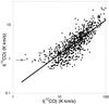 |
Fig. A.1 Scatter plot of I(13CO) versus I(12CO) for the 734 sources detected in 13CO. The solid line is a linear fit to the data points in the figure and indicates that I(12CO) is, on average, a good linear tracer of H2 column density for I(12CO) > 5 K km s-1. The 1-σ noise is indicated on two representative low intensity points; on the scale of this figure it can be seen that the signal-to-noise ratio is very high except for a few of the weakest 12CO points. The detection limits are given in Table 2. |
All Tables
All Figures
|
Fig. 1 A schematic of the distribution of lines of sight for the GOT C+ Galactic plane survey where they are represented by solid arrows superimposed on an artist’s impression of the Galaxy (R. Hurt, Courtesy NASA/JPL-Caltech). Each arrow represents many lines of sight as they are too dense to display. The longitudinal spacings are indicated on the figure and regions of different angular spacing are separated by dashed arrows. The finest spacing is 0.87° towards the innermost Galaxy and increases outwards. The red lines mark the range l = 270° to 57° of data analyzed in this paper. The area covered from l = 90° to 270°, which is mostly in the outer Galaxy, is only about 20% to 25% of the area of the disk and consequently a larger angular spacing is used, varying from 4.5° at 90° and 270° to 12° near 180°. |
| In the text | |
|
Fig. 2 Spectra along three representative lines of sight from the GOT C+ inner Galaxy survey showing Tmb, the main-beam temperature, versus Vlsr. The upper panel for each line of sight shows the [C ii] spectrum along with the fits derived from the Gaussian decomposition (shown in red). The lower panel for each line of sight shows the corresponding H i in black, 12CO in blue, 13CO in red, and C18O in green. The scalings for Tmb are shown in each panel. |
| In the text | |
|
Fig. 3 Number distribution of [C ii] sources as a function of Galactic radius for b = 0°, ± 0.5° combined, and ± 1° combined. With increasing b there are fewer sources and their distribution skews closer to the solar radius because the line of sight at some distance away from the solar system is above the plane where there a fewer sources; see text for details. |
| In the text | |
|
Fig. 4 Distribution of [C ii] sources as a function of Galactic radius for clouds as characterized by the presence or absence of CO isotopologues. All values of Galactic latitude, b, are included in this figure. |
| In the text | |
|
Fig. 5 Distribution of CO sources without detectable [C ii] as a function of Galactic radius; all values of Galactic latitude, b, are included in this figure. |
| In the text | |
|
Fig. 6 Scatter plot of I([C ii]) versus I(H i) for all [C ii] sources. The straight lines are predicted I([C ii]) for low density atomic H i diffuse clouds as a function of I(H i) (which is proportional to the H i column density) for four different characteristic pressures from P = 2000 K cm-3 to 6000 K cm-3. This pressure range covers predicted values for the diffuse clouds from Rgal ~ 10 kpc to ~4 kpc, with 3000 K cm-3 characteristic of the solar radius. It is clear that the vast majority of the GOT C+ [C ii] sources require an additional source of [C ii] emission other than the diffuse atomic gas. The 1-σ noise for I([C ii]) is indicated on three representative low intensity points; those for I(H i) are too small to be visible on this figure and have been omitted. It can be seen on the scale of this figure that the S/N is high for most of points in this scatter plot. |
| In the text | |
|
Fig. 7 Schematic of the [C ii] emission from different types of clouds along the line of sight. |
| In the text | |
|
Fig. 8 Dependence of T-1exp( − 91.25/T), which is proportional to the relative excitation rate to the |
| In the text | |
|
Fig. 9 IH2([C ii]), the intensity of [C ii] in the H2 layer plotted against I(13CO) on a log-log scale. There is a trend towards larger IH2([C ii]) with increasing I(13CO). The solid line shows a linear fit to the data, IH2([C ii]) = 1.08 + 0.49 I(13CO), which appears curved when transformed to the log-log plot shown here. The 1-σ noise for IH2([C ii]) is indicated on three points; those for I(13CO) are too small to be visible on this figure and have been omitted. It can be seen on the scale of this figure that the S/N is high for most of points in this scatter plot. |
| In the text | |
|
Fig. 10 Distribution of the column density of the CO-dark H2 gas layer in all [C ii] sources in the GOT C+ inner Galaxy survey. |
| In the text | |
|
Fig. 11 Distribution of column density of the CO-traced gas, N(CO-traced H2) in [C ii] sources. |
| In the text | |
|
Fig. 12 Distribution of the column density of the CO-dark H2 gas layer sorted by type of cloud in the GOT C+ inner Galaxy survey: (top) diffuse molecular clouds; (middle) transition molecular clouds; and, (bottom) dense molecular clouds. |
| In the text | |
|
Fig. 13 Distribution of total H2 column density for different types of clouds: (top left) diffuse molecular clouds with no CO; (top right) 12CO transition molecular clouds; (bottom left) dense molecular clouds with 13CO; and (bottom right) all [C ii] sources. Note that the vertical scale is different in the last panel. |
| In the text | |
|
Fig. 14 Fraction by mass of CO-dark H2 gas for different classes of clouds: (upper left) diffuse molecular clouds, the [C ii] sources with no CO; (upper right) transition molecular clouds, [C ii] sources with only 12CO; (lower left) dense molecular clouds, with 13CO and no C18O; and, (lower right) dense molecular clouds with 13CO and a dense C18O core (or cores). |
| In the text | |
|
Fig. 15 Fraction by mass of CO-dark H2 gas for all the [C ii] sources. |
| In the text | |
|
Fig. 16 Column density of CO-dark H2 gas for all CO sources as a function of the total hydrogen column density Ntot = N(H i) + 2N(H2). The curves are N(CO-dark H2) calculated from the models of Visser et al. (2009) as discussed in the text. The central curve (dashed line) is the 100-point means of their model shown in the right panel of their Fig. 7. The top curve (dotted line) is the lower limit on the solutions for N(CO), which yields a maximum for N(CO-dark H2), and the bottom curve (solid line) is the upper limit on N(CO), which yields a minimum for N(CO-dark H2), as a function of N(H2) for the range of parameter space used in their models. |
| In the text | |
|
Fig. 17 Fraction by mass of CO-dark H2 gas for all sources as a function of the total hydrogen column density Ntot = N(H i) + 2N(H2): diffuse molecular clouds (red °), 12CO transition molecular clouds (blue ×), and 13CO dense molecular clouds (black △). The curves on the left are f(CO-dark H2) calculated from the models of Visser et al. (2009) as discussed in the text. The central curve (dashed blue line) is the 100-point means of their model shown in the right panel of their Fig. 7. The top curve (dotted red line) is the lower limit on the solutions for N(CO), while the bottom curve (solid black line) is the upper limit on N(CO) as a function of N(H2) for the range of parameter space used in their models. On the right side we plot the few values of f(CO-dark H2) calculated by Wolfire et al. (2010) for massive clouds for different values of metallicity relative to the solar value, Z′ = 0.5 (red line), 1.0 (blue line), and 1.9 (black line). |
| In the text | |
|
Fig. 18 Distribution of f(CO-dark H2) in CO sources with detectable [C ii] averaged over rings as a function of Galactic radius. |
| In the text | |
|
Fig. A.1 Scatter plot of I(13CO) versus I(12CO) for the 734 sources detected in 13CO. The solid line is a linear fit to the data points in the figure and indicates that I(12CO) is, on average, a good linear tracer of H2 column density for I(12CO) > 5 K km s-1. The 1-σ noise is indicated on two representative low intensity points; on the scale of this figure it can be seen that the signal-to-noise ratio is very high except for a few of the weakest 12CO points. The detection limits are given in Table 2. |
| In the text | |
Current usage metrics show cumulative count of Article Views (full-text article views including HTML views, PDF and ePub downloads, according to the available data) and Abstracts Views on Vision4Press platform.
Data correspond to usage on the plateform after 2015. The current usage metrics is available 48-96 hours after online publication and is updated daily on week days.
Initial download of the metrics may take a while.