| Issue |
A&A
Volume 560, December 2013
|
|
|---|---|---|
| Article Number | A16 | |
| Number of page(s) | 16 | |
| Section | Stellar structure and evolution | |
| DOI | https://doi.org/10.1051/0004-6361/201322480 | |
| Published online | 28 November 2013 | |
A comparison of evolutionary tracks for single Galactic massive stars⋆
LUPM, Université Montpellier 2, CNRS, Place Eugène Bataillon 34095 Montpellier France
e-mail:
This email address is being protected from spambots. You need JavaScript enabled to view it.
Received: 13 August 2013
Accepted: 22 October 2013
Abstract
Context. The evolution of massive stars is not fully understood. The relation between different types of evolved massive stars is not clear, and the role of factors such as binarity, rotation or magnetism needs to be quantified.
Aims. Several groups make available the results of 1D single stellar evolution calculations in the form of evolutionary tracks and isochrones. They use different stellar evolution codes for which the input physics and its implementation varies. In this paper, we aim at comparing the currently available evolutionary tracks for massive stars. We focus on calculations aiming at reproducing the evolution of Galactic stars. Our main goal is to highlight the uncertainties on the predicted evolutionary paths.
Methods. We compute stellar evolution models with the codes MESA and STAREVOL. We compare our results with those of four published grids of massive stellar evolution models (Geneva, STERN, Padova and FRANEC codes). We first investigate the effects of overshooting, mass loss, metallicity, chemical composition. We subsequently focus on rotation. Finally, we compare the predictions of published evolutionary models with the observed properties of a large sample of Galactic stars.
Results. We find that all models agree well for the main sequence evolution. Large differences in luminosity and temperatures appear for the post main sequence evolution, especially in the cool part of the Hertzsprung-Russell (HR) diagram. Depending on the physical ingredients, tracks of different initial masses can overlap, rendering any mass estimate doubtful. For masses between 7 and 20 M⊙, we find that the main sequence width is slightly too narrow in the Geneva models including rotation. It is (much) too wide for the (STERN) FRANEC models. This conclusion is reached from the investigation of the HR diagram and from the evolution of the surface velocity as a function of surface gravity. An overshooting parameter α between 0.1 and 0.2 in models with rotation is preferred to reproduce the main sequence width. Determinations of surface abundances of carbon and nitrogen are partly inconsistent and cannot be used at present to discriminate between the predictions of published tracks. For stars with initial masses larger than about 60 M⊙, the FRANEC models with rotation can reproduce the observations of luminous O supergiants and WNh stars, while the Geneva models remain too hot.
Key words: stars: massive / stars: evolution
STAREVOL and MESA tracks are only available at the CDS via anonymous ftp to cdsarc.u-strasbg.fr (130.79.128.5) or via http://cdsarc.u-strasbg.fr/viz-bin/qcat?J/A+A/560/A16
© ESO, 2013
1. Introduction
Massive stars (M > 8 M⊙) are born as O and B stars on the zero age main sequence (ZAMS). After a few million years, they evolve off the main sequence to become either (red) supergiants or Wolf-Rayet stars, depending on their initial mass. They may go through a phase during which they are seen as luminous blue variables (LBV), blue or yellow supergiants. Beyond this qualitative scenario, little is known about the evolution of massive stars. In particular, the detailed relations between stars of different types is poorly constrained. Very massive and luminous H-rich WN stars are probably core-H burning objects (Martins et al. 2008; Crowther et al. 2010). They may become LBVs when they evolve towards the red part of the Hertzsprung-Russell (HR) diagram (Smith & Conti 2008). At lower masses (M ~ 50 M⊙), Crowther & Bohannan (1997) and Martins et al. (2007) provided relations between mid-O supergiants and several types of WN and WC stars. These evolutionary sequences remain partial, and do not exist for the entire upper HR diagram.
Main ingredients of the evolutionary models.
Stellar evolutionary models have been developed to explain and predict the physical properties of massive stars. The effective temperature and luminosity they predict are used to build tracks followed by stars of different initial masses in the HR diagram. These predictions are confronted to observations to test the input physics. Hamann et al. (2006) studied the WN stars in the Galaxy and concluded that the models of Meynet & Maeder (2003) are able to account for the global properties of WN stars. However, some quantitative problems exist, especially regarding the number of early and late WN stars. Similarly, the ratio of WC to WN stars provides a test of evolutionary models. According to the classical scenario, WC stars represent a more advanced state of evolution than WN stars, simply because of mass loss: as evolution proceeds, mass is removed by stellar winds and deeper layers are unveiled. It takes more time to reach deeper layers, and consequently these layers bear the imprint of the nucleosynthesis occurring at later stages of evolution. Neugent & Massey (2011) showed that the ratio WC/WN is correctly reproduced by the models of Meynet & Maeder (2003) at low metallicity. This is not the case at higher metallicity (see also Neugent et al. 2012) where evolutionary models predict too few WC stars. Hunter et al. (2008) studied the nitrogen content of B stars in the Large Magellanic Cloud and found that single standard stellar evolutionary models could account for the properties of roughly two thirds of the sample, the remaining objects being unexplained by current single star tracks with rotation. The results were confirmed by the calculations of Brott et al. (2011b). Nonetheless, Maeder et al. (2009) cautioned that many parameters could affect the surface abundances and that they needed to be considered.
Indeed, evolutionary calculations rely on various prescriptions to describe the physical processes driving the evolution, and these prescriptions may vary from code to code. The most important ingredients/processes to be considered are convection and its related properties (such as overshooting), mass loss (Chiosi & Maeder 1986), chemical composition (and the relative abundance of the various species considered in the models) and of course initial mass. Rotation is another key ingredient, since it affects the internal structure, the physical properties (temperature, luminosity), the surface chemical appearance and the lifetimes of stars (Maeder & Meynet 2000b). Several prescriptions usually exist to treat a given physical process in evolutionary codes. As a consequence, the outputs depend on the input physics. Since evolutionary calculations are a crucial tool to link the observed properties of stars to their physical state and evolution, it is important to understand the limitations and uncertainties associated with evolutionary models.
Properties of the 20 M⊙ model computed with different codes, without rotation, and evaluated at four different evolutionary phases.
In this paper, we present a comparison of various predictions of the evolution of massive stars computed with different codes. Our goal is to highlight the uncertainties in the outputs of evolutionary calculations, especially concerning the HR diagram. We focus on calculations for Galactic stars. In Sect. 2 we describe the different codes and models we have used in our comparisons. We then present a study of the uncertainties associated with the assumptions in the input physics (Sect. 3). In the same section, we also compare the evolutionary tracks predicted by the different codes. In Sect. 4 we confront the predictions of published grids of models to the observed properties of massive stars in the Galaxy. We highlight the limitations of each grid. Finally, we summarize our main conclusions in Sect. 5.
2. Stellar evolution models
To achieve our goal of comparing stellar evolution tracks of massive stars, we have used four databases of stellar evolution tracks presented in Bertelli et al. (2009), Brott et al. (2011a), Ekström et al. (2012), Chieffi & Limongi (2013) and we computed models using the STAREVOL code (Decressin et al. 2009) and the MESA code (Paxton et al. 2011, 2013). We recall here the main ingredients and physical parameters used in each case since they may differ largely and these differences appear to affect the evolutionary tracks. Table 1 summarizes the main inputs for each code.
2.1. STERN stellar evolution code (Brott et al. 2011a)
We first make use of the grid of stellar evolution models published by Brott et al. (2011a). The computations have been performed with the code fully described in Heger et al. (2000). In the following, we will refer to this code as the STERN code.
Solar reference chemical composition. Brott et al. (2011a) adopt tailored reference chemical abundances for their models of LMC, SMC and Galactic massive stars based on the solar abundances of Asplund et al. (2005) with a modification of the C, N, O, Mg, Si and Fe abundances. This results in unusual chemical mixtures described in Tables 1 and 2 of their paper. Their adopted values for the metal mass fraction Z is 0.0088, 0.0047 and 0.0021 for the Galaxy, the LMC and the SMC respectively. The Galactic metallicity is about half the value used by the other codes (see below). The initial helium content is Y = 0.264. The OPAL radiative opacities of Iglesias & Rogers (1996) are used in the calculations.
Convection. They use the Ledoux criterion1 to determine the extension of the convective regions, and model convection according to the mixing length theory with αMLT = 1.5. The mixing length is the length over which a displaced element conserves its properties, and the mixing length parameter αMLT, is the ratio of the mixing length to the local pressure scale height HP. The zones which are stable according to the Ledoux criterion but unstable according to the Schwarzschild criterion are considered to be semi-convective. Semi-convection is included as in Langer et al. (1983) with αsc = 1. Finally Brott et al. calibrate an additional classical overshooting parameter to adjust the evolution of the rotation velocity as a function of surface gravity of a 16 M⊙ model at LMC metallicity (see Sect. 4.1). This parameter is applied to their entire grid and results in an extension of the convective cores beyond the limit defined by the Ledoux criterion by dover = 0.335Hp.
Mass loss. Mass loss is implemented following a combination of prescriptions or recipes that are specific for each evolutionary phase of massive stars. Brott et al. (2011a) use Vink et al. (2000, 2001) (ṀV) for winds of early O and B-type stars. A switch to Ṁ by Nieuwenhuijzen & de Jager (1990) (ṀNdJ) is operated at Teff< 22 000 K (bi-stability jump temperature) whenever ṀV<ṀNdJ. Another switch is operated for the Wolf-Rayet phase, and Ṁ by Hamann et al. (1995) is adopted as soon as Ys ≥ 0.7 (Ys is the surface helium abundance). For intermediate values of Ys, an interpolation between the Vink et al. mass loss rates and the Wolf-Rayet mass loss rates reduced by a factor 10 is performed. Brott et al. use a metallicity scaling of the mass loss by a factor (Fesurf/Fe⊙)0.85 based on the solar iron abundance from Grevesse et al. (1996) (ϵ(Fe) = 7.50), which is higher than that of their models (ϵ(Fe) = 7.40). For the rotating models, they also apply the correction factor  to the mass loss rate (Vcrit is the critical velocity).
Rotation and rotation-induced mixing. The effects of the centrifugal acceleration on the stellar structure equations is considered according to Kippenhahn et al. (1970). The transport of angular momentum and chemical species is treated in a diffusive way following the formalism by Endal & Sofia (1978) as described in Heger et al. (2000). Eddington-Sweet circulation, dynamical and secular shear, and axisymmetric (GSF) instabilities contribute to the transport of both angular momentum and chemical species. The formalism they use relies on two efficiency factors (free parameters): fc = 0.0228 which reduces the contribution to the rotation-induced hydrodynamical instabilities in the total diffusion coefficient, and fμ = 0.1 which regulates the inhibiting effect of chemical gradients on the rotational mixing. The values of these parameters are calibrated on observations. They are fully described in Eqs. (53) and (54) of Heger et al. (2000).
In addition to that, the action of magnetic fields on the transport of angular momentum only is included through the highly debated Tayler-Spruit dynamo (Spruit 2002) following Petrovic et al. (2005).
2.2. Geneva stellar evolution code (Ekström et al. 2012)
We also use the grid published by Ekström et al. (2012), and summarize briefly the main physical ingredients used to compute the models provided in that paper.
Solar reference chemical composition. It is based on Asplund et al. (2005) with a modification of the Ne abundance according to Cunha et al. (2006). Their adopted metals mass fraction is Z = 0.014 resulting from a solar calibration. The initial helium content is Y = 0.266. The OPAL radiative opacities of Iglesias & Rogers (1996) are used.
Convection. They use the Schwarzschild criterion to define the convective regions. Convection is modelled following the mixing-length formalism with αMLT = 1.6. For models with M > 40 M⊙ the mixing length parameter is computed using the density height scale instead of the pressure height scale with αMLT = 1 following Maeder (1987).
They also include classical overshoot at the convective core edge with αover = 0.1. This parameter corresponds to the ratio between the extension of the convective core beyond the value resulting from the Schwarzschild criterion to the local pressure scale height. dover = 0.1HP is calibrated to reproduce the width of the main sequence in the mass range 1.35−9 M⊙. Semi-convection is not modelled.
Mass loss. Mass loss is implemented following a combination of prescriptions or recipes chosen to best represent mass loss of massive stars along their evolution. Ekström et al. use the stellar winds prescriptions from Vink et al. (2000, 2001) when log (Teff) > 3.9. A switch to de Jager et al. (1988) mass loss formulae is operated when the models reach log (Teff) < 3.9 and then to Crowther (2000) as they evolve into the red supergiant phase. For the Wolf-Rayet phases (log (Teff) > 4 and XS ≤ 0.4 − XS being the surface hydrogen abundance), they use Nugis & Lamers (2000) or Gräfener & Hamann (2008).
Mass loss rates are scaled according to Maeder & Meynet (2000a) for the rotating models.
For the most massive models (M > 15 M⊙), in order to account for the supra-Eddington mass loss during the red supergiant phase, they multiply Ṁ by a factor of 3 whenever the luminosity in the envelope becomes 5 times larger than the Eddington luminosity.
Rotation and rotation-induced mixing. The modification of the stellar structure equations by the centrifugal acceleration is taken into account following Meynet & Maeder (1997). The transport of angular momentum and of nuclides due to meridional circulation and turbulent shear is self-consistently included following the formalism by Zahn (1992) and Maeder & Zahn (1998). The prescriptions used for the turbulent diffusion coefficients are from Zahn (1992) for the horizontal component and from Maeder (1997) for the vertical component. Convective regions are assumed to rotate as solid-bodies. No additional transport due to the presence of magnetic fields is included.
2.3. FRANEC stellar evolution code (Chieffi & Limongi 2013)
Chieffi & Limongi (2013) reported on the inclusion of rotation in the FRANEC code and have computed a grid of massive stellar evolution models with and without rotation.
Solar reference chemical composition. The models are computed using the heavy element solar mixture from Asplund et al. (2009). The initial global metallicity and helium content are Z = 0.01345 and Y = 0.265. The associated opacities are from OPAL for radiative opacities.
Convection. Convection is treated following the MLT formalism and convective limits are defined using the Schwarzschild criterion except for the H burning shell appearing at the beginning of the core He burning phase, for which the Ledoux criterion is applied (see Limongi et al. 2003). The mixing length parameter adopted is not given, but should be of α = Λ/Hp = 2.3 according to Straniero et al. (1997). Classical overshooting is included with a value of dover = 0.2Hp.
Mass loss. They use the mass loss prescriptions of Vink et al. (2000, 2001) for the blue supergiant phase, switching to de Jager et al. (1988) when log (Teff) < 3.9, and Nugis & Lamers (2000) for the WR phase. The mass loss during the red supergiant phase is enhanced according to van Loon et al. (2005). Mass loss of rotating models is also enhanced as in the STERN code, following Heger et al. (2000).
Rotation and rotation-induced mixing. The modification of the stellar structure equations by the centrifugal acceleration and the transport of angular momentum and of nuclides are the same as in the Geneva code.
The impact of the mean molecular weight gradients on the transport of both angular momentum and nuclides is regulated by the use of a free parameter fμ defined by  . Chieffi & Limongi adopted fμ = 0.03. This value is calibrated to ensure that at solar metallicity, the stars in the mass range 15−20 M⊙ settling on the main sequence with an equatorial velocity of 300 km s-1 will increase their surface nitrogen abundance by a factor of ≈3 by the time they reach the TAMS.
Convective regions are assumed to rotate as solid-bodies.
No additional transport due to the presence of magnetic fields is included.
2.4. Padova stellar evolutionary code (Bertelli et al. 2009)
The evolutionary models for massive stars computed with the Padova code are described in Bertelli et al. (2009). Additional information regarding the code can be found in Bono et al. (2000) and Pietrinferni et al. (2004, 2006). Rotation is not included in the grid of Bertelli et al. (2009).
Solar reference chemical composition. The metals mass fraction adopted for their solar-metallicity models is Z = 0.017. We used the models with Y = 0.26 (several values are available). The OPAL radiative opacities of Iglesias & Rogers (1996) are used. A global scaling of the relative element mass fractions is made compared to the mixture of Grevesse et al. (1993) on which the OPAL tables are based. For very high temperatures (log T > 8.7), the opacities of Weiss et al. (1990) are used.
Convection. They adopt the formalism of the mixing length theory with αMLT = 1.68, calibrated on solar models. Stability is set by the Schwarzschild criterion. Overshooting is taken into account with a free parameter corresponding to the ratio of the true extent of the convection core to the convection core radius defined by the Schwarzschild criterion. The notable difference in the Padova code is that this parameter expresses the extent of overshooting across (and not above) the border of the convective core (as set by the Schwarzschild criterion). A value of 0.5 for the overshooting parameter is adopted. Overshooting below the convective envelopes is also accounted for with a parameter equal to 0.7.
Semi-convection is considered to be negligible for massive stars models.
Mass loss. The mass loss prescriptions of de Jager et al. (1988) are used for all phases of evolution. A metallicity scaling of radiatively driven winds is taken into account according to Kudritzki et al. (1989) (i.e. Ṁ ∝ Z0.5).
2.5. STAREVOL (Decressin et al. 2009)
A detailed description of the STAREVOL code can be found in Siess et al. (2000); Siess (2006); Decressin et al. (2009). The models computed for the present study were obtained using the STAREVOL v3.30 which includes a number of updates with respect to previous descriptions of the code2. For the present study we have adopted a setup close to that used in the Geneva grid.
Solar reference chemical composition. We use Asplund et al. (2009) with OPAL tabulated opacities modified accordingly. At low temperature we use the Ferguson et al. (2005) opacities computed for the Asplund et al. 2009 solar composition. The adopted solar metallicity is thus Z = 0.0134. The initial helium content is Y = 0.277. No further modification of the abundances is made. When computing models for non-solar metallicities, a simple proportionality is applied.
Convection. The Schwarzschild criterion is used to define the convective regions. Convection is modelled following the mixing-length formalism as described in Kippenhahn & Weigert (1990). The mixing length parameter αMLT = 1.64 is calibrated for the solar model. In some models, we have included classical overshoot at the edge of convective regions with αover = 0.1 or 0.2.
Mass loss. For massive stars (M > 7 M⊙) with log (Teff) > 3.9 we apply the prescriptions from Vink et al. (2000, 2001), which we change to (a) de Jager et al. (1988) when the models evolve to the red and have their temperature drop below log (Teff) = 3.9 and then to Crowther (2000) as they evolve into the red supergiant phase, (b) to Reimers (1975) for models in the mass range 7−12 M⊙ when they evolve off the main sequence, (c) to Nugis & Lamers (2000) for those models that experience a Wolf-Rayet phase (e.g. with log (Teff) > 4 and XS ≤ 0.4).
The mass loss is down-scaled by a factor (Z/Z⊙)0.5 for non-solar metallicity models. We have included the correction to the mass loss of rotating massive stars according to Maeder & Meynet (2001).
Rotation and rotation-induced mixing. The modification of the stellar structure equations due to centrifugal acceleration in rotating models is taken into account following Kippenhahn et al. (1970). The expression for the effective temperature following this formalism is implemented as described in Appendix A of Meynet & Maeder (1997). In addition to this, the transport of angular momentum and of nuclides is as in the Geneva and FRANEC codes. The prescriptions used for the turbulent diffusion coefficients are from Zahn (1992) for the horizontal component and from Talon & Zahn (1997) for the vertical component.
Convective regions are assumed to rotate as solid-bodies.
No additional transport due to the presence of magnetic fields is included.
2.6. MESA code (Paxton et al. 2011)
MESA3 is a public distribution of modules for experiments in stellar astrophysics. The computation of evolutionary models is possible with the module “star” of the distribution. An exhaustive description of the code is available in Paxton et al. (2011) and Paxton et al. (2013). We have computed dedicated evolutionary models for 7, 9, 15, 20, 25, 40 and 60 M⊙ stars. Both non-rotating and rotating (initial equatorial velocity of 200 km s-1) models have been calculated.
Solar reference chemical composition. We have adopted a value of Y = 0.26 and Z = 0.014 in our calculations. MESA uses OPAL opacities from Iglesias & Rogers (1996). The relative mass fraction of metals in the OPAL composition is based on the solar composition of Grevesse et al. (1993), Grevesse & Sauval (1998) or Asplund et al. (2009). The user can select any of these compositions. A global scaling with Z is made when non-solar metallicity models are computed.
Convection. The standard mixing length formalism as defined by Cox (1968) is used to treat convection as a diffusive process in MESA. The onset of convection is ruled by the Schwarzschild criterion. In our calculations, we used αMLT = 2.0. Although it is available, we did not include semi-convection in our models. Convective overshooting is treated as a diffusive process following the formalism of Herwig (2000). The overshooting diffusion coefficient (Dov) is related to the MLT diffusion coefficient (Dconv) through  where f is a free parameter. Unless stated otherwise, we have adopted f = 0.01 in our calculations.
Mass loss. A mixture of prescriptions is used to account for mass loss in the various phases of evolution. The recipe of Vink et al. (2001) is used for Teff > 10 000 K and X(H) > 0.4. For the same temperature range, but lower H content (X(H) < 0.4), the mass loss rates of Nugis & Lamers (2000) are implemented. For Teff < 10 000 K, the values of de Jager et al. (1988) are used. It is possible to scale these prescriptions by a constant factor. For hot star, it is a way to take the metallicity dependence of mass loss rates into account (see Sect. 3.1).
Rotation and rotation-induced mixing. The geometrical effects of rotation are implemented following the formalism of Kippenhahn et al. (1970). The transport of angular momentum and chemical species through meridional circulation and hydrodynamical instabilities turbulence is treated as a purely diffusive process, following the Endal & Sofia (1978) formalism as in the STERN code. The efficiency factor (see Sect. 2.1) have the following values: fc = 1/30, similar to the theoretical value of Chaboyer & Zahn (1992), and fμ = 0.1. We did not include magnetism in our computation (although the formalism of Spruit 2002 is implemented in MESA and can be switched on).
3. Code predictions and uncertainties
In this section, we perform comparisons between the results of calculations performed with the six codes described above. We focus on the evolutionary tracks in the HR diagram. We first compare standard tracks (i.e. without rotation) in order to test the various implementations of the basic physics. We subsequently investigate the effects of rotation.
3.1. Effects of physical ingredients on evolutionary tracks
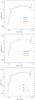 |
Fig. 1 Effects of opacities (top), overshooting (middle) and mass loss (bottom) on 20 M⊙ evolutionary tracks. The computations have been performed with the code MESA. In the upper panel, different solar heavy elements mixtures are used, for the same initial metal fraction (Z = 0.014). GN93 refers to Grevesse et al. (1993), GS98 to Grevesse & Sauval (1998) and AGS09 to Asplund et al. (2009). |
In Fig. 1 we illustrate the effect of modifying the opacities, the overshooting and the mass loss on the evolution of a M = 20 M⊙ model from the ZAMS to the terminal age helium main sequence (TAHeMS). We have used both the MESA and STAREVOL codes to compute the evolutionary sequences. We mainly discuss the MESA models in this section (the results obtained using STAREVOL are very similar).
The top panel illustrates the effect of different heavy elements solar mixtures on the opacities. The solar composition of Grevesse et al. (1993) and Asplund et al. (2009) are relatively similar: the C, N, O and Ne abundances do not differ by more than ~0.05 dex. The Grevesse & Sauval (1998) abundances are on average 0.10−0.15 dex larger. In Fig. 1, we see that the main effects of different solar composition on the opacities is reflected in the post main sequence evolution. On the main sequence, the luminosity variations are negligible, while beyond the terminal age main sequence (TAMS) the differences vary between 0.01 and 0.02 dex depending on the temperature.
The middle panel of Fig. 1 shows the effect of overshooting. The calculations have been performed for a diffusive overshooting with a parameter f equal to 0, 0.01 and 0.02 as indicated on the figure. Overshooting is included only in the convective regions related to H burning. Qualitatively, the effect of an increasing overshooting is the lengthening of the main sequence phase. As a result of the larger extension of the convective core, a larger amount of hydrogen is available for helium production in the core. Quantitatively, the main sequence duration is 8.60 Myr for f = 0.01 and 9.06 Myr for f = 0.02. This corresponds to an increase of 9%. As a consequence of the longer main sequence duration for larger overshooting, the star exits the core H burning phase at a lower effective temperature (by 2500 K), and at a higher luminosity (increase of 0.05 dex) when f increases from 0.01 to 0.02. If the overshooting parameter is not constrained, a degeneracy in the evolutionary status of a star located close to the end of the main sequence can appear. Depending on the tracks used and the amount of overshooting, it can be identified as a core H burning object close to end of the main sequence, or as a post main sequence object. Beyond the main sequence, models with stronger overshooting evolve similarly but at higher luminosities.
The bottom panel of Fig. 1 illustrates the effect of mass loss rates on evolutionary paths. In addition to the track with the standard mass loss rate, two additional tracks with mass loss rates globally scaled by a factor 0.33 and 0.10 are shown. As expected, the main sequence is barely affected. The reason is the low values of the mass loss rates during this phase for the initial mass of 20 M⊙ considered here. For the standard track (dashed blue line) the mass at the end of the main sequence is 19.66 M⊙, corresponding to a loss of only 1.7% of the initial mass over 8.60 Myr. The mass drops to 18.26 M⊙ in the next Myr (time to reach the bottom of the red giant branch). On average, the mass loss rate is thus 35 times larger in the post-main sequence phase compared to the main sequence. To first order, the effect of mass loss can be understood as a simple shift to lower luminosity. Since the luminosity is directly proportional to some power-law of the mass (the exponent being around 1.0−2.0 depending on the mass, e.g. Kippenhahn & Weigert 1990), a reduction of the mass immediately translates into a reduced luminosity. This is what we observe in Fig. 1. Quantitatively, a reduction by a factor close to 3 (10) in the mass loss rates corresponds to a maximum increase in luminosity of ~0.01 (0.03) dex. The changes are larger for more massive stars since mass loss rates are also higher.
The prescriptions of mass loss rates for massive stars suffer from several uncertainties. The presence of clumping in hot stars winds has lead to a reduction of the mass loss rates by a factor of roughly 3 (Puls et al. 2008). But this value is still debated, reduction up to a factor of 10 being sometimes necessary to reproduce observational diagnostics (Bouret et al. 2005; Fullerton et al. 2006). For the cool part of the evolution of a massive star, the very nature of the mass loss mechanism is still not clear. Mauron & Josselin (2011) have shown that the mass loss rates of de Jager et al. (1988) are still valid. But for a given luminosity, the scatter in mass loss rates is large (up to a factor 10). The uncertainties in the mass loss rates thus translate into uncertainties of the order of 0.02 dex in the luminosity of evolutionary tracks beyond the TAMS.
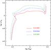 |
Fig. 2 Effect of metallicity on a 20 M⊙ model computed with MESA. |
Figure 2 highlights the well documented effects of metallicity (e.g. Meynet & Maeder 2003). We have computed models for three different metallicities: the solar value (Z = 0.014) and the extreme values encountered in the Galaxy according to the study of HII regions by Balser et al. (2011) − Z = 1.5 Z⊙ and Z = 1/2.5 Z⊙. No scaling of the mass loss rates was applied in order to extract the effect of metallicity on the internal structure and evolution. A lower metal content corresponds to a lower opacity, which in turn translates into a higher luminosity. On average, a reduction of the metal content by a factor of two translates into an increase in luminosity by 0.005−0.010 dex on the main sequence and by 0.03−0.05 dex beyond.
Assuming a typical uncertainty on the luminosity of ±0.02 dex (opacity effect), ±0.04 dex (overshooting effect), ±0.01 dex (mass loss effect), ±0.03 dex (metallicity effect) and simply adding quadratically the errors, we obtain a global uncertainty of about ±0.05 dex on the luminosity of a MESA track. The values we adopted are typical of the uncertainties at the end of the main sequence and around Teff = 10 000 K. An uncertainty of 0.05 dex on the luminosity is equivalent to an uncertainty of about 6% on the distance of the star. On the main sequence, the uncertainty on the luminosity is lower than ±0.02 dex.
We have computed a second set of these models using the STAREVOL code, and we also find that the choice of the overshooting and of the metallicity are the ones affecting the most the luminosity. The global uncertainty on the 20 M⊙ track computed with STAREVOL is of ±0.06 dex around Teff = 10 000 K, of the same order than that found for MESA models. In Fig. 3, we display the envelope corresponding to the global intrinsic error for the MESA and STAREVOL models of 20 M⊙. For both sets of models, the shape of the envelope is similar. The uncertainty is maximum at temperatures around 10 000 K (in the core He burning phase, see Table 2). The uncertainty on the luminosity at a given effective temperature is not symmetrical with respect to the reference track shown in dashed line. These envelopes illustrate the intrinsic uncertainties of a given evolutionary track.
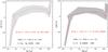 |
Fig. 3 Region occupied by the evolutionary tracks of 20 M⊙ models computed with MESA (left) and STAREVOL (right) with different opacities, metallicities, mass loss rates and overshooting parameters. The dashed red line shows the track of the standard model, with the parameters as indicated on the figure (the overshooting parameter − ov − is not defined in the same way in both codes, hence the different values). The shaded envelope defines a rough global intrinsic uncertainty on 20 M⊙ models. |
We have performed the same type of calculations and comparisons on a M = 7 M⊙ model. The effect of mass loss is negligible (changes in luminosity smaller then 0.01 dex). Different chemical mixtures and their effect on opacities translates to uncertainties <0.05 dex on the luminosity. They are roughly similar to the effects seen in the M = 20 M⊙ star. A change in metallicity from solar to 1/2.5 solar corresponds to an increase in luminosity by 0.1 dex. Hotter temperatures are also obtained. The effect is larger than in the M = 20 M⊙ model. Finally, the largest effect on the evolutionary track of the M = 7 M⊙ model is due to changes in the overshooting parameter. Variations in luminosity by 0.10−0.15 dex are observed beyond the main sequence. The effect of overshooting dominates the uncertainty on the M = 7 M⊙ evolutionary track. The global uncertainty on the luminosity of the M = 7 M⊙ model amounts to 0.2 dex, which is equivalent to an error of 30% on the distance.
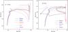 |
Fig. 4 Evolutionary tracks for M = 20 M⊙ (left) and M = 40 M⊙ (right), without rotation. For the M = 40 M⊙ case, no Padova track exists. |
3.2. Comparison between codes
In this section we make direct comparisons between the six codes presented in Sect. 2. We focus on the M = 20 M⊙ track corresponding to a late O star on the main sequence. Table 2 gathers the effective temperature, luminosity and age at four different evolutionary phases, for the six types of models. The 40 M⊙ track is also briefly presented at the end of this section.
Figure 4 (left) shows the evolutionary tracks of classical (no rotation included) 20 M⊙ model at solar metallicity. On the main sequence there is an overall good agreement between the outputs of the different codes. The STERN track is overluminous and bluer than the others which is expected from its lower metallicity (Z = 0.0088 vs. Z = 0.014−0.017 for all the other tracks). The TAMS of the Geneva, STAREVOL and MESA models is located in the same region of the HR diagram as can also be verified from Table 2. However, the age at the TAMS is quite different for the Geneva Model, which is younger by ≈0.7 Myr compared to the STAREVOL and MESA models. A difference in age at the TAMS with no associated difference in Teff nor luminosity may indicate differences in the nuclear physics.
The characteristic hook at the end of the main sequence occurs at lower temperatures for the FRANEC, Padova and STERN models. The larger amount of overshooting, hence the size of the H core, is responsible for these differences (see Table 1). From Table 2, we also see that FRANEC and Padova models reach the TAMS later (by ~0.5 Myr) compared to MESA and STAREVOL models, which is consistent with having a larger reservoir of fuel to be consumed during the hydrogen core burning phase. On the other hand, and surprisingly, the STERN model is even younger than all the models except the Geneva one, when it reaches the TAMS. The lower metal content might lead to a higher core temperature and consequently to a faster hydrogen burning via the CNO reactions. At the end of the main sequence, an age spread of 1.3 Myr (15%) is observed between the six codes.
Beyond the main sequence, the differences between the various codes are larger. The Geneva/Starevol/MESA tracks are still rather similar in the post main sequence evolution, with differences in luminosity usually lower than 0.05 dex. The red supergiant part of the STAREVOL model is located redwards compared to that of the MESA and Geneva models. The reason for this behaviour is attributed to a combination of differences in the mixing length parameter, the opacities and the equation of state. The Padova and FRANEC models reach the TAMS with larger luminosities due to the stronger overshoot, and see their luminosity subsequently decrease to a large amount (0.3 dex in the case of the FRANEC model). This behaviour is also observed in the STERN model. The Padova, STERN and FRANEC models reach  = 4.87, 4.77 and 4.71 respectively at the bottom of the red giant branch, compared to the = 5.00−5.05 reached by the MESA, STAREVOL and Geneva models. The decrease of the total luminosity during the Hertzsprung gap results from a subtle balance between the core contraction, the energy generation by the H shell surrounding the core, the mean molecular weight gradient profile and the opacity of the surface layers. For the Padova, STERN and FRANEC models, the thermal instability of the envelope (triggered by the above conditions) seems to be stronger, leading to a larger overall reduction of the luminosity. Given that the detailed structures associated with these tracks are not all available, it is difficult to be more precise concerning the different paths followed by the tracks presented here.
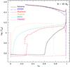 |
Fig. 5 Effective temperature as a function of central helium mass fraction for a M = 20 M⊙ model computed with the six codes considered in this study. |
The beginning of the helium core burning phase (ZAHeMS) is defined as the time at which the central helium mass fraction starts to decrease from its maximum value reached after the central hydrogen burning phase. The ZAHeMS starts at Teff ~ 25 000 K for most models, except the Padova (Teff = 15 657 K) and the STERN (Teff = 5388 K) ones. We attribute the very different temperature of the STERN models to the large overshooting and the inclusion of magnetism. The temperatures at the TAHeMS differ by 350 K at most. This is a large difference (10%), affecting the interpretation of the properties of red supergiants (e.g. Levesque et al. 2005; Davies et al. 2013). The tracks from FRANEC and Padova tracks present a blue hook similar to what is observed during core helium burning for lower masses.
The large differences in the post main sequence evolution can also be seen in Fig. 5 where we show the evolution of effective temperature as a function of core helium mass fraction (YC). The MESA and STAREVOL tracks spend most of the helium burning phase at temperatures larger than 10 000 K. 40% of the helium burning phase takes place at hot temperatures in the Geneva model. The subsequent evolution takes place mainly at low Teff. In the FRANEC model, almost all the helium burning is done in the cool part of the HR diagram. Finally, the Padova model features a blue loop so that helium burning is first done at low Teff before finishing at Teff> 10 000 K.
To summarize, the evolution of the M = 20 M⊙ model becomes more uncertain as temperature decreases (i.e. as the star evolves), with a wider spread in luminosity in the HR diagram. This type of differences also exists for lower mass stars not analyzed here4, and reveals the uncertainty of the He-burning phases understanding and modelling. The length of the main sequence depends on the treatment of overshooting, as illustrated in Sect. 3.1. Differences in luminosity up to 0.3 dex (a factor of 2) and in temperatures up to 10% are observed in the coolest phases of evolution.
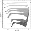 |
Fig. 6 Envelopes of evolutionary paths for M =7, 9, 15, 20, 25, 40 and 60 M⊙ taking into account the predictions of the codes studied in this paper. Rotation is not included. The envelopes for the 7 and 9 M⊙ models do not include FRANEC since no tracks is available for these masses. The Padova models do not exist for 40 and 60 M⊙. For the 40 and 60 M⊙ tracks, the envelope encompasses only the redward evolution (the Wolf-Rayet phases are not included). |
Figure 4 (right) shows the evolutionary tracks for a M = 40 M⊙ star. Padova models for such a mass are not available (the grid of Bertelli et al. 2009 stops at M = 20 M⊙). The Geneva, MESA and STAREVOL models are very similar during the H and He burning phases. The FRANEC track has the same path as the Geneva/MESA/STAREVOL tracks on the main sequence. Beyond that, its luminosity is about 0.05 to 0.08 dex lower until it reaches the red part of the HR diagram where it drops by another 0.12 dex before rising again by 0.25 dex and starting its blueward evolution towards the Wolf-Rayet phase. The behaviour is very different from the other models since once in the red part of the HR diagram, the luminosity increases instead of decreasing. This behaviour is tentatively attributed to the size of the H-rich envelope that develops in the FRANEC model when the luminosity drops. This envelope reaches 15 M⊙ at the lowest effective temperature. For comparison, in the MESA model it represents at most about 10 M⊙. The STERN track is more luminous than all other tracks on the main sequence. It does not show the characteristic hook revealing the end of the convective core H burning phase. This feature is very peculiar in the STERN track and is attributed to the combination of the very large overshooting parameter and the inclusion of magnetism (see Sect. 4.1).
In Fig. 6 we present a summary of the comparison between the available standard tracks. For each mass, we present envelopes encompassing the tracks produced by the six codes. These envelopes are defined from the ZAMS to temperatures of about 3000 K. For sake of clarity, the subsequent evolution (back to the blue) of the most massive objects (M > 40 M⊙) is not taken into account to create these envelopes. Such envelopes provide a first guess of the uncertainty on the evolutionary tracks for specific masses. The main sequence phase is relatively well defined with the major uncertainties being encountered at the exhaustion of central hydrogen, when the track makes a hook in the HR diagram. For the masses shown in Fig. 6, there is no overlap. The same conclusion remains for the post main sequence evolution above 40 M⊙. For the lower masses there is a degeneracy on the mass at low temperatures where the envelopes defining the possible location for a specific mass overlap. The overlap is the largest in the coolest phases (below 5000 K). Severe degeneracies in the initial masses appear. For instance, a star with log (Teff) = 3.6 and = 4.2 can be reproduced by tracks of stars with initial masses between 7 and 15 M⊙. The corresponding stellar ages are thus very different (see also Martins et al. 2012b).
The global intrinsic uncertainty within models computed with the same stellar evolution code (0.05 dex at most for a 20 M⊙ model) is much lower than the uncertainty coming from the use of tracks computed with different stellar evolution codes (0.4 dex at maximum for M = 20 M⊙, see Fig. 6). The uncertainty is in both cases larger beyond the TAMS, and it appears that no clear consensus exists on the position of lower end of the red giant branch nor on the temperature of the red giant branch itself, making it very difficult to draw trustful conclusions when comparing effective temperatures and luminosities obtained from spectroscopic analysis with predictions of evolutionary tracks for yellow/red supergiants. Age determinations are also very uncertain.
3.3. Rotation
The effects of rotation on evolutionary tracks of massive stars have been described in details in the literature. We refer to Maeder & Meynet (2000b) and Langer (2012) for reviews of the main effects. To summarize, the effects of rotation can be broadly described as follows:
-
geometrical effects: rapid rotation tends to flatten stars, the equatorial radius becoming larger than the polar radius. As a consequence the equatorial gravity is smaller than the polar gravity. According to the Von Zeipel theorem (von Zeipel 1924), the effective temperature at the pole is larger.
-
Effects on transport processes: rotation triggers various instabilities and fluid motions in the stellar interior (e.g. meridional circulation, shear instability) which transport angular momentum and chemical species between the stellar core and the surface. Consequently, the surface abundances and internal distribution of species are strongly affected by rotation.
-
Effect on mass loss rate: rotation modifies the surface temperature and gravity as described above. Since radiatively driven winds are directly related to these quantities (Castor et al. 1975), mass loss rates are also affected. Maeder & Meynet (2000a) showed that on average, they increase with the ratio of rotational velocity to critical rotational velocity.
A direct consequence of the mixing processes on the evolution of a star is an increase of the duration of the core hydrogen burning phase. Because of mixing, material above the central convective core is brought to the center, leading to a refuelling of the core hence to an extension of the hydrogen core burning phase duration. The effect is qualitatively the same as overshooting. This is somewhat counterbalanced by the larger luminosity of rotating tracks, caused by a different radial profile of the mean molecular weight. A higher luminosity translates into a shorter nuclear burning timescale. But this effect is smaller than the effect of mixing, so that on average, rotation leads to longer nuclear burning sequences (by 10−20% for the main sequence). Rotating stars thus end their main sequence with larger luminosities than non rotating stars.
In Fig. 7 we show the envelopes of tracks for M = 20 M⊙. The dark grey one corresponds to rotating models, the light grey one to non rotating models. The envelopes have been defined from the tracks computed with STERN, FRANEC, the Geneva code, STAREVOL and MESA. We have excluded the Padova tracks since they do not include rotation. The MESA and STAREVOL tracks have been computed assuming an initial surface equatorial velocity of 200 and 233 km s-1 respectively. The STERN and FRANEC tracks have an initial velocity of 300 km s-1. The Geneva tracks have been computed for a ratio of initial to critical rotation of about 0.4, corresponding, with their definition of the critical velocity, to about 250 km s-1 at the equator.
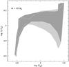 |
Fig. 7 Uncertainty on the location of the evolutionary path for a 20 M⊙ stellar model with (dark grey envelope) and without (light grey delimited by dashes lines) rotation. We have considered tracks generated by five different codes (Geneva, STERN, FRANEC, MESA and Starevol) with similar (yet not exactly the same) initial rotation rates. |
The widening of the main sequence described above is visible in Fig. 7: the dark grey region extends over a wider luminosity range from the ZAMS to the TAMS. Beyond the main sequence, the envelope of the rotating models is wider than that of the non-rotating models immediately after the TAMS, and becomes subsequently narrower at temperatures below ~20 000 K. In the Hertzsprung gap (5000 <Teff< 20 000 K), the less luminous of the rotating tracks are overluminous by about 0.1 dex in compared to the non rotating tracks. The width of the envelope remains large in the coolest phases: 0.2 dex at log Teff = 3.7. Since we are using models with different rotational velocities (between 200 and 300 km s-1) the width of the corresponding envelope is most likely affected by this dispersion of velocities and is probably an upper limit. If all models had been computed with the same initial velocity, the spread in luminosity would be slightly smaller.
The global uncertainty associated with the choice of a specific grid of stellar evolution models is reduced beyond the ZAMS when considering models including rotation. This is essentially due to the fact that the decrease in luminosity after the TAMS when the tracks crosses the Hertzsprung gap, is much less important in the rotating models generated with STERN and FRANEC codes. We may attribute it to the larger mass loss and efficient mixing.
4. Comparisons with observational results
After comparing results of calculation with different codes, we now turn to comparisons to observational data. From now on, we use only the publicly available grids of tracks of Brott et al. (2011a), Ekström et al. (2012) and Chieffi & Limongi (2013). All include rotational mixing.
4.1. The main sequence width
In Fig. 8 we show a HR diagram with OB stars and the evolutionary tracks of the three public grids. The tracks are truncated so that only the part corresponding to a hydrogen mass fraction higher than 0.60 is shown5. This is already a high value for O stars, corresponding to He/H = 0.35 by number. The stellar parameters for the comparison stars result from detailed analysis with atmosphere models or from calibrations according to spectral types. In that case, the calibrations of Martins et al. (2005a) have been used to assign an effective temperature. A bolometric correction was subsequently computed following Martins & Plez (2006). Extinction was calculated from B − V. The distance to the stars (taken from parallaxes when available, or from cluster membership) finally lead to the magnitudes and thus, with the bolometric correction, to the luminosity. The data concerning the comparison stars have been taken from the following studies: Massey & Johnson (1993), McErlean et al. (1999), Vrancken et al. (2000), Walborn et al. (2002), Lyubimkov et al. (2002), Levenhagen & Leister (2004), Martins et al. (2005b, 2008, 2012a,b), Crowther et al. (2006a,b, 2010), Melena et al. (2008), Searle et al. (2008), Markova & Puls (2008), Martins et al. (2008), Hunter et al. (2009), Lefever et al. (2010), Liermann et al. (2010), Negueruela et al. (2010), Przybilla et al. (2010), and Bouret et al. (2012). In the following, we will assume that the main sequence is populated by stars of luminosity class V and IV. This is a reasonable assumption for stars below ~40 M⊙ but certainly an oversimplification for stars above 40 M⊙ for which the spectroscopic luminosity class is not necessarily matching the internal evolutionary status (a luminous star with a strong mass loss can still be burning hydrogen in its core and already have the appearance of a supergiant because of its wind).
The upper panel of Fig. 8 shows the Geneva tracks with initial rotation on the ZAMS between 180 and 270 km s-1 depending on the initial mass. The width of the main sequence (between the solid and short dashed - long dashed lines) corresponds well to the position of main sequence stars below ~7 M⊙. The extension of the main sequence might be slightly too small for masses between 7 and 25 M⊙ (compared with the location of red triangles and pentagons, that is stars with luminosity classes of IV and V). The main sequence width is larger when rotation is included, as expected.
In the middle panel of Fig. 8 we show the HR diagram built using the tracks of Brott et al. (2011a) for V sin i = 300 km s-1. The main sequence for models including rotation is wider than for the Geneva models. For masses of 10−15 M⊙, the main sequence extension corresponds to the area populated by luminosity class V, IV and III objects. Bright giants and supergiants are located beyond the main sequence. All giant stars (green squares) being included in the main sequence width, the core H-burning phase in the Brott et al. models is too extended. The models without rotation have a narrower main sequence, in better agreement with the position of dwarfs and sub-giants below ~15 M⊙. The main difference between the Geneva and STERN tracks is attributed to the overshooting parameter (α = 0.335 for STERN versus 0.1 for Geneva). The larger overshooting in the Brott et al. models translates into a wider main sequence. This is particularly true above ~30 M⊙ where all blue supergiants are within the main sequence width. Even if some supergiant stars can in principle still be main sequence objects at high luminosity, it is unlikely that all of them are core-H burning objects, indicating that an overshooting of 0.335 is too large for stars with masses above 20 M⊙.
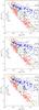 |
Fig. 8 Comparison between evolutionary tracks (black lines) and the location of OB stars in the HR diagram. The evolutionary tracks are from Ekström et al. (2012) (top), Brott et al. (2011a) (middle) and Chieffi & Limongi (2013) (bottom). They are shown for hydrogen mass fraction lower than 0.60 for clarity. The short dashed − long dashed line connects the cooler edge of the main sequence for the different models and defines the TAMS. The dotted lines is the same for the non-rotating models. Different symbols correspond to different luminosity classes. Filled symbols correspond to stars for which the stellar parameters have been determined through a tailored analysis, while open symbols are for stars with parameters taken from calibrations according to their spectral type. The data sources are listed in the text, Sect. 4.1. |
Finally, the bottom panel of Fig. 8 shows the FRANEC models of Chieffi & Limongi (2013). Unfortunately, this grid only includes models for masses larger than 13 M⊙ so we focus on the HR diagram above this mass. Between 13 and 20 M⊙, the main sequence width appears to be a little wider than the extension of the region where luminosity class V and IV stars are located. Most giants (green squares) are within the predicted main sequence band. Non rotating models better account for the observed extension of the main sequence. Beyond 20 M⊙ and up to 40 M⊙ the MS width remains roughly constant and includes many supergiants. It might thus be too wide. As for the STERN models, this may be due to the overshooting parameter (α = 0.2 for Chieffi & Limongi). We note the peculiar behaviour of the non rotating models above 40 M⊙: the core H burning phase extends to cooler temperatures than the models including rotation.
From the HR diagram, we thus conclude that moderate values of the overshooting parameter (α < 0.2) in models with initial rotational velocities of 250−300 km s-1 correctly reproduce the main sequence width. For models without rotation, a larger amount of overshooting is required to compensate for the reduction of the main sequence width.
There are few determinations of the strength of overshooting in the literature, and they provide conflicting results. Ribas et al. (2000) used eclipsing binaries to show that α increases with mass, but Claret (2007) found that α = 0.2 could reproduce correctly the properties of 3 < M < 30 M⊙ stars. Using asteroseismology, Briquet et al. (2007) determined α = 0.44 ± 0.07 for the B2IV star θ Oph and Briquet et al. (2011) obtained α = 0.1 ± 0.05 for the O9V star HD 46202. One of the main reasons for these differences is that it is usually the extent of the convective core that is constrained from observations. From this size, the overshooting distance is determined by subtraction of the convective core predicted by models in absence of overshooting. This core size depends on the input physics and thus varies from model to model, implying that the estimates of the overshooting distance also depend on the uncertainties of the evolutionary models. Although it relies on a physical effect, overshooting can be partly viewed as an adjustment variable to correctly reproduce the extension of stellar convective cores that are deduced from observations. Keeping this limitation in mind, we can test the values of overshooting adopted in the various codes.
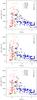 |
Fig. 9 Projected rotational velocity as a function of surface gravity. The symbols have the same meaning as in Fig. 8. Top: evolutionary tracks from Brott et al. (2011a). Middle: evolutionary tracks from Ekström et al. (2012). Bottom: evolutionary tracks from Chieffi & Limongi (2013). The vertical dashed line is a guideline located at log g = 3.45. |
The large overshooting parameter adopted by Brott et al. (2011a) results from the comparison of the projected rotational velocity to the surface gravity of massive stars in LMC clusters. High gravity objects show a wide range of rotational velocities, while low log g stars have V sin i< 100 km s-1. The transition occurs at about log g = 3.2 in the LMC stars and corresponds to the rapid inflation of the star after the end of the core-H burning phase. The larger radius immediately translates into a lower velocity. Brott et al. (2011a) calibrated the overshooting parameter of their 16 M⊙ model to reproduce this sudden drop.
Figure 9 shows the V sin i − log g diagram for the stars used to build the HR diagram of Fig. 8. Only the stars for which both the projected rotational velocity and surface gravity are available are included in Fig. 9. As expected, a clear transition is seen at log g = 3.45. Above this value, velocities span the range 0−400 km s-1, while below only the lowest velocities (<100 km s-1) are observed. Main sequence objects (red triangles) are all located on the left part of the transition, while most supergiants (blue circles) are found on the right side. This is qualitatively consistent with the results of Hunter et al. (2009) and Brott et al. (2011a). However, the value we obtain for the transition gravity at solar metallicity is larger than that obtained for the LMC by these authors: 3.45 versus 3.2. The overshooting used by Brott et al. to reproduce the properties of LMC stars is too high for Galactic targets. This is illustrated in the upper panel of Fig. 9 where we see that the Brott et al’s tracks have a terminal main sequence (identified by the loop in the tracks) at log g = 2.9−3.2 for masses between 5 and 20 M⊙. The large overshooting increases the core-H burning phase, resulting in a bigger star and thus a lower gravity at the hydrogen core exhaustion. The middle panel of Fig. 9 shows the behaviour of the Geneva models. In the 5−20 M⊙ range, the TAMS is located at log g = 3.25−3.60, in better agreement with the observational data. However, the 5 and 9 M⊙ tracks have a TAMS at log g slightly too large compared to the position of luminosity class V stars. A value of α equal to 0.1 is a little too low to reproduce the bulk of main sequence stars. The bottom panel presents the tracks from Chieffi & Limongi (2013) in the mass range 13 M⊙ to 60 M⊙. The overshoot parameter used for these models is d/Hp = 0.2, and we see an intermediate behaviour compared to the two other families of tracks, as expected for this intermediate value of overshooting. The TAMS is located at log g = 3.0−3.2, at gravities too low compared to the observations.
Let us note that the Geneva and FRANEC tracks (Figs. 9b and c) behave similarly beyond the TAMS (in particular the 40 M⊙ track) and only cover the slowest supergiants (blue circles), with predicted surface velocities of less than 40 km s-1for log g < 3.0. The models from the STERN grid on the other hand experience a weaker braking and conserve a more rapid rotation beyond. They better reproduce the observed distribution of rotation velocities of supergiants. The treatment of rotation induced mixing and angular momentum evolution in the STERN code is different from that implemented in the Geneva and FRANEC codes, which might explain these differences in the evolution of the surface equatorial velocity.
In conclusion, an overshooting parameter a little larger than 0.1 is required to have a convective core extension able to account for the observed width of the main sequence for Galactic OB stars.
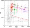 |
Fig. 10 C/H as a function of N/H. The symbols correspond to results from spectroscopic analysis from Martins et al. (2008); Hunter et al. (2009); Przybilla et al. (2010); Nieva & Simón-Díaz (2011); Firnstein & Przybilla (2012); Bouret et al. (2012). The evolutionary tracks for various masses between 15 and 60 M⊙ are taken from Ekström et al. (2012) (black), Brott et al. (2011a) (red) and Chieffi & Limongi (2013) (magenta). |
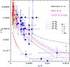 |
Fig. 11 Same as Fig. 10 on a wider scale to show abundances of evolved objects. The stars analyzed by Hunter et al. (2009) have been omitted for clarity. |
4.2. Surface carbon and nitrogen content
Rotation modifies the surface abundances because of the induced mixing processes. Surface abundances are thus important diagnostics to see how realistic is the treatment of rotation in evolutionary models. In Figs. 10 and 11 we compare the C/H and N/H ratios predicted by the models to those determined for OB stars. The symbols correspond to Galactic stars analyzed by means of quantitative spectroscopic analysis. The evolutionary tracks of Brott et al. (2011a), Ekström et al. (2012) and Chieffi & Limongi (2013) are shown. They span a mass range between 15 and 60 M⊙. OB stars on the main sequence have an initial carbon content between 5.0 × 10⁻⁵ and 2.6 × 10⁻⁴. We note that values lower than 2.0 × 10⁻⁴ are only obtained in the study of Hunter et al. (2009). The other studies of main sequence stars (Przybilla et al. 2010; Nieva & Simón-Díaz 2011; Firnstein & Przybilla 2012) all find C/H larger than 2.0 × 10⁻⁴, consistent with the solar reference value of Grevesse et al. (2010).
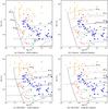 |
Fig. 12 Same as Fig. 8 but focusing on the upper part of the HR diagram. The orange squares correspond to WNh stars. We have used stars for which stellar parameters determined from spectroscopic analysis are available. In the upper (lower) panels the Geneva (FRANEC) models are shown. The tracks have been plotted for X(He) < 0.75 which corresponds to He/H ~ 0.8 by number. Left: tracks with rotation. Right: non rotating tracks. |
The Brott et al. (2011a) tracks have an initial composition roughly corresponding to the average of the B stars of Hunter et al. (2009). The few B stars of Hunter et al. with evidence for N enrichment are rather well accounted for by these tracks. On the other hand, the OB stars analyzed by Przybilla et al. (2010), Nieva & Simón-Díaz (2011) and Firnstein & Przybilla (2012) cannot be reproduced by the Brott et al. tracks. The Ekström et al. (2012) and Chieffi & Limongi (2013) predictions are better (although on average slightly too carbon rich for the Geneva models) to account for the initial composition and the evolution of these stars. One may wonder whether the samples of Hunter et al. (2009) and Przybilla et al. (2010)/Nieva & Simón-Díaz (2011)/Firnstein & Przybilla (2012) are taken from environments with different metallicities. Hunter et al. (2009) focused on NGC 6611 towards the Galactic Center, and NGC 3293/NGC 4755 at Galactic longitudes of 285° and 303° and distances close to 2 kpc. The stars of Przybilla et al. (2010)/Nieva & Simón-Díaz (2011)/Firnstein & Przybilla (2012) are mostly from the solar neighborhood. We thus do not expect strong metallicity differences among the stars shown in Fig. 10. The reason for the differences in C abundance at the beginning of the evolution between the two sets of stars is thus not clear. It might be related to the methods used to determine the stellar parameters and the surface abundances.
Turning to Fig. 11, we see that evolved OB stars are well reproduced by the Ekström et al. and Chieffi & Limongi models, although the number of stars with good C and N abundances is still too small to draw firm conclusions. The Brott et al. (2011a) tracks have a too low carbon content at a given N/H because of the initial offset discussed above.
These comparisons indicate that accurate abundance determinations are necessary before the predictions of evolutionary models regarding surface composition can be tested at depth. The reason for the difference between the study of Hunter et al. on the one hand, and of Nieva, Przybilla, Firnstein and collaborators on the other hand needs to be understood before preference can be given to a set of tracks.
4.3. The upper HR diagram
In this section, we focus on the upper HR diagram, i.e. at luminosities larger than 3 × 10⁵ L⊙. The only publicly available tracks including rotation for stars with masses larger than 60 M⊙ are provided by the Geneva group and Chieffi & Limongi (2013). In Fig. 12 we plot the evolutionary tracks of Ekström et al. (2012) and Chieffi & Limongi in the upper and lower panels respectively. Only the part of the tracks with a surface helium mass fraction smaller than 0.75 is shown. This is equivalent to a number ratio He/H of about 0.8. This value is the largest determined for most WNh stars (Hamann et al. 2006; Martins et al. 2008; Liermann et al. 2010).
We first focus on the Geneva models. The WNh stars and the most luminous supergiants cannot be accounted for by the evolutionary tracks with rotation of Ekström et al. (2012). The 60, 85 and 120 M⊙ tracks turn to the blue almost immediately after the ZAMS (Fig. 12, upper left panel). The 60 M⊙ track later comes back to the red part of the HRD, but at that time it is depleted in hydrogen, while the comparison stars all still contain a significant fraction of hydrogen. The 85 and 120 M⊙ tracks do not come back to the right of the ZAMS and cannot reproduce the position of the WNh stars. We thus conclude that the solar metallicity tracks with rotation of Ekström et al. (2012) do not account for the most massive stars and thus should not be used for comparisons with normal stars with masses above 60 M⊙. The Geneva tracks are computed for  where veq and vcrit are the equatorial velocity and the break-up velocity. For stars with M > 60 M⊙ the initial velocity is ~280 km s-1. Although not extreme, and in spite of the rapid drop of the rotational velocity with age (see Fig. 10 of Ekström et al. 2012) the fast initial rotation may explain the blueward evolution of the most massive models. This behaviour is similar to that of quasi-chemically homogeneous tracks (Maeder 1987; Langer 1992).
For comparison, we show on the upper right panel of Fig. 12 the Geneva non rotating tracks, with the same cut in helium mass fraction. This time, the 60, 85 and 120 M⊙ models cross the region occupied by the most luminous supergiants and the WNh stars. With a low or moderate helium content, they can thus reproduce the existence of these very luminous objects. One can conclude that the current Geneva rotating tracks are probably computed with a too high initial rotational velocity to explain the existence of most of the Galactic WNh and early O supergiants. The tracks by Meynet & Maeder (2003) include rotation with an initial equatorial velocity of 300 km s-1 and have Z = 0.020. They are super-solar according to the current calibration of solar abundances (Z = 0.014). They do not show the rapid blueward evolution just after the ZAMS seen in the Ekström et al. tracks. They better account for the very massive stars, as exemplified by the studies of Hamann et al. (2006) and Martins et al. (2008). Since the initial rotational velocity in the Meynet & Maeder (2003) tracks is larger than in the Ekström et al. (2012) models, we attribute the different behaviour to the metallicity difference.
Levesque et al. (2012) used the evolutionary tracks including rotation of Ekström et al. (2012) to compute population synthesis models. They concluded that the inclusion of rotation lead to a significant increase of the ionizing flux in young stellar population. The main reason is a shift towards higher luminosities of the tracks when rotation is included (see Sect. 3.3). In the earliest phases, the presence of stars with masses in excess of 60 M⊙ also contributes to the larger ionizing flux, since as illustrated above, the tracks predict much higher temperature when rotation is included. As discussed by Levesque et al. (2012), their predictions are probably biased towards populations with larger than average rotational velocities. In view of the direct comparison between evolutionary tracks and position of Galactic massive stars in the HR diagram, we confirm that the Ekström et al. (2012) tracks should be used with a good recognition that they are relevant for fast rotating objects.
Coming back to the lower panels of Fig. 12, we see that the models of Chieffi & Limongi do not suffer from the same problems as the Geneva models. The 60 and 80 M⊙ tracks including rotation evolve classically towards the red part of the HR diagram. They all have initial rotation of about 250 km s-1 similar to that of the 20 M⊙ and 40 M⊙ models from Ekström et al. (2012) as can be see from Fig. 9. They can account for stars as luminous as 106 L⊙. The 120 M⊙ track also evolves redwards, but turns back to the blue at log Teff = 4.54. Many of the luminous WNh stars can be explained by this track. Only three objects at log Teff = 4.4 are not reproduced by the FRANEC tracks. But the 120 M⊙ non-rotating track (lower right panel of Fig. 12) extends down to such temperatures. Since the rotation of massive stars spans a range of values, it is possible that some objects are slow rotators. Unfortunately, it is difficult to measure rotation velocities in WNh stars since their spectrum is dominated by lines formed above the photosphere, in the wind.
We thus conclude that overall the Chieffi & Limongi tracks better reproduce the population of luminous O supergiants and WNh stars in the HR diagram. For the most luminous stars, it appears that non-rotating tracks may give a better fit to the observations than rotating ones when only considering the position in the HR diagram. The difference between the FRANEC and Geneva computations are: 1) a larger overshooting and mixing length parameter and 2) the inclusion of efficiency factors in the treatment of rotation in the study of Chieffi & Limongi. The mass loss rates in the temperature range of interest are the same. Since the Geneva models are very different with and without rotation, we tend to attribute the differences with the FRANEC models to the second point listed above. The efficiency factors of Chieffi & Limongi reduce the impact of rotation on the diffusion coefficients. Qualitatively, they could limit the strong effects of rotation seen in the grid of Ekström et al. (2012).
5. Conclusion
We have performed a comparison of evolutionary models for massive stars in the Galaxy. The published grids of Bertelli et al. (2009), Brott et al. (2011a), Ekström et al. (2012) and Chieffi & Limongi (2013) have been used. We have also computed additional models with the codes STAREVOL (Decressin et al. 2009) and MESA (Paxton et al. 2013). Our goal was to estimate and highlight the uncertainties in the output of these models. Our conclusions are:
-
Evolutionary tracks in the HR diagram are sensitive to the adopted solar composition mixture, metallicity, the amount of overshooting and the mass loss rate. The extension of the convective core, due to overshooting and/or rotation-induced mixing, and the adopted initial metallicity are the major sources of uncertainty on the determined luminosity on the main sequence and during the core He burning phase. Within one set of stellar evolution models, we estimate a global intrinsic uncertainty on the luminosity of about ±0.05 dex for a star with an initial mass of 20 M⊙. This uncertainty is lower when studying main sequence stars. This uncertainty translates into an error of about 6% on the distance, and may rise up to an error of 30% on the distance of lower mass red supergiants (typically stars with initial mass of 7 M⊙).
-
The evolutionary tracks computed with the six different codes agree reasonably well for the main sequence evolution. Beyond that, large differences appear. They are the largest at low effective temperature. In the red part of the HR diagram, evolutionary tracks with different initial masses and computed with different codes can overlap. The difference on the luminosity of a star located near the red giant branch can be as large as 0.4 dex depending on the stellar evolution models adopted, which makes the estimate of ages and initial masses for red supergiants extremely uncertain.
-
Comparison of the tracks of Brott et al. (2011a), Ekström et al. (2012) and Chieffi & Limongi (2013) with the properties (Teff, luminosity) of a large number of OB and WNh stars in the Galaxy indicate that in the mass range 7−20 M⊙ the Ekström et al. tracks have a slightly too narrow main sequence width, while the Brott et al. and Chieffi & Limongi tracks have a too wide one. This is due to the overshooting parameters used. These results are confirmed by the analysis of the distribution of rotational velocities as a function of log g for Galactic stars with various spectral types. A clear drop in rotational velocities is observed at log g = 3.45, at larger gravity than that observed for LMC stars studied by Hunter et al. (2008). An overshooting parameter slightly above 0.1 is required to reproduce this trend.
-
Measurements of surface abundances of carbon and nitrogen are currently too uncertain to help constrain evolutionary models.
-
Stars with initial masses higher than about 60 M⊙ are not accounted for by the Ekström et al. tracks with rotation. They bend to the blue part of the HR diagram quickly after leaving the zero age main sequence, and do not reproduce the position of the WNh and luminous blue supergiants. Models provided by Chieffi & Limongi give a much better fit to the observations. Non rotating tracks of both grids can reproduce the position of the most luminous objects.
Future analysis of surface abundances of large samples of Galactic OB stars will provide critical constraints on evolutionary models and the treatment of rotation. Better prescriptions of mass loss rates for a wide variety of stars are also required to improve the predictions of evolutionary models.
For a plasma described by a general equation of state, the Ledoux stability criterion is given by  with
with  and
and  , μ being the mean molecular weight. When there are no chemical gradients, ∇μ = 0 and the Schwarzschild stability criterion is recovered: ∇rad < ∇ad.
The updates concern opacities and reference solar abundances, as well as mass-loss prescriptions.
See for instance the results presented at the workshop “The Giant Branches” held in Leiden in May 2009 − http:///www.lorentzcenter.nl/lc/web/2009/324/program.php3?wsid=324
This value is chosen so that the end of the main sequence for the 40 M⊙ track is visible.
Acknowledgments
We warmly thank the MESA team for making their code freely available (http://mesa.sourceforge.net/). We thank Marco Limongi and Alessandro Chieffi for kindly providing their models and associated information. We aknowledge the comments and suggestions of an anonymous referee. We thank Georges Meynet, Daniel Schaerer, Sylvia Ekström, Cyril Georgy, Selma de Mink, Hugues Sana for interesting discussions. This study was supported by the grant ANR-11-JS56-0007 (Agence Nationale de la Recherche).
References
- Asplund, M., Grevesse, N., & Sauval, A. J. 2005, in Cosmic Abundances as Records of Stellar Evolution and Nucleosynthesis, eds. T. G. Barnes III, & F. N. Bash, ASP Conf. Ser., 336, 25 [Google Scholar]
- Asplund, M., Grevesse, N., Sauval, A. J., & Scott, P. 2009, ARA&A, 47, 481 [NASA ADS] [CrossRef] [Google Scholar]
- Balser, D. S., Rood, R. T., Bania, T. M., & Anderson, L. D. 2011, ApJ, 738, 27 [NASA ADS] [CrossRef] [Google Scholar]
- Bertelli, G., Nasi, E., Girardi, L., & Marigo, P. 2009, A&A, 508, 355 [NASA ADS] [CrossRef] [EDP Sciences] [Google Scholar]
- Bono, G., Caputo, F., Cassisi, S., et al. 2000, ApJ, 543, 955 [NASA ADS] [CrossRef] [Google Scholar]
- Bouret, J.-C., Lanz, T., & Hillier, D. J. 2005, A&A, 438, 301 [NASA ADS] [CrossRef] [EDP Sciences] [Google Scholar]
- Bouret, J.-C., Hillier, D. J., Lanz, T., & Fullerton, A. W. 2012, A&A, 544, A67 [NASA ADS] [CrossRef] [EDP Sciences] [Google Scholar]
- Briquet, M., Morel, T., Thoul, A., et al. 2007, MNRAS, 381, 1482 [NASA ADS] [CrossRef] [Google Scholar]
- Briquet, M., Aerts, C., Baglin, A., et al. 2011, A&A, 527, A112 [NASA ADS] [CrossRef] [EDP Sciences] [Google Scholar]
- Brott, I., de Mink, S. E., Cantiello, M., et al. 2011a, A&A, 530, A115 [NASA ADS] [CrossRef] [EDP Sciences] [Google Scholar]
- Brott, I., Evans, C. J., Hunter, I., et al. 2011b, A&A, 530, A116 [NASA ADS] [CrossRef] [EDP Sciences] [Google Scholar]
- Castor, J. I., Abbott, D. C., & Klein, R. I. 1975, ApJ, 195, 157 [NASA ADS] [CrossRef] [Google Scholar]
- Chaboyer, B., & Zahn, J.-P. 1992, A&A, 253, 173 [NASA ADS] [Google Scholar]
- Chieffi, A., & Limongi, M. 2013, ApJ, 764, 21 [NASA ADS] [CrossRef] [Google Scholar]
- Chiosi, C., & Maeder, A. 1986, ARA&A, 24, 329 [NASA ADS] [CrossRef] [Google Scholar]
- Claret, A. 2007, A&A, 475, 1019 [NASA ADS] [CrossRef] [EDP Sciences] [Google Scholar]
- Cox, J. P. 1968, Principles of stellar structure − Vol. 1: Physical principles; Vol.2: Applications to stars (New York: Gordon and Breach) [Google Scholar]
- Crowther, P. A. 2000, A&A, 356, 191 [NASA ADS] [Google Scholar]
- Crowther, P. A., & Bohannan, B. 1997, A&A, 317, 532 [NASA ADS] [Google Scholar]
- Crowther, P. A., Hadfield, L. J., Clark, J. S., Negueruela, I., & Vacca, W. D. 2006a, MNRAS, 372, 1407 [NASA ADS] [CrossRef] [Google Scholar]
- Crowther, P. A., Lennon, D. J., & Walborn, N. R. 2006b, A&A, 446, 279 [NASA ADS] [CrossRef] [EDP Sciences] [Google Scholar]
- Crowther, P. A., Schnurr, O., Hirschi, R., et al. 2010, MNRAS, 408, 731 [NASA ADS] [CrossRef] [Google Scholar]
- Cunha, K., Hubeny, I., & Lanz, T. 2006, ApJ, 647, L143 [NASA ADS] [CrossRef] [Google Scholar]
- Davies, B., Kudritzki, R.-P., Plez, B., et al. 2013, ApJ, 767, 3 [NASA ADS] [CrossRef] [Google Scholar]
- de Jager, C., Nieuwenhuijzen, H., & van der Hucht, K. A. 1988, A&AS, 72, 259 [NASA ADS] [Google Scholar]
- Decressin, T., Mathis, S., Palacios, A., et al. 2009, A&A, 495, 271 [NASA ADS] [CrossRef] [EDP Sciences] [Google Scholar]
- Ekström, S., Georgy, C., Eggenberger, P., et al. 2012, A&A, 537, A146 [NASA ADS] [CrossRef] [EDP Sciences] [Google Scholar]
- Endal, A. S., & Sofia, S. 1978, ApJ, 220, 279 [NASA ADS] [CrossRef] [Google Scholar]
- Ferguson, J. W., Alexander, D. R., Allard, F., et al. 2005, ApJ, 623, 585 [NASA ADS] [CrossRef] [Google Scholar]
- Firnstein, M., & Przybilla, N. 2012, A&A, 543, A80 [NASA ADS] [CrossRef] [EDP Sciences] [Google Scholar]
- Fullerton, A. W., Massa, D. L., & Prinja, R. K. 2006, ApJ, 637, 1025 [NASA ADS] [CrossRef] [Google Scholar]
- Gräfener, G., & Hamann, W.-R. 2008, A&A, 482, 945 [NASA ADS] [CrossRef] [EDP Sciences] [Google Scholar]
- Grevesse, N., & Sauval, A. J. 1998, Space Sci. Rev., 85, 161 [NASA ADS] [CrossRef] [Google Scholar]
- Grevesse, N., Noels, A., & Sauval, A. J. 1993, A&A, 271, 587 [NASA ADS] [Google Scholar]
- Grevesse, N., Noels, A., & Sauval, A. J. 1996, in Cosmic Abundances, eds. S. S. Holt, & G. Sonneborn, ASP Conf. Ser., 99, 117 [Google Scholar]
- Grevesse, N., Asplund, M., Sauval, A. J., & Scott, P. 2010, Ap&SS, 328, 179 [NASA ADS] [CrossRef] [Google Scholar]
- Hamann, W.-R., Koesterke, L., & Wessolowski, U. 1995, A&A, 299, 151 [NASA ADS] [Google Scholar]
- Hamann, W.-R., Gräfener, G., & Liermann, A. 2006, A&A, 457, 1015 [NASA ADS] [CrossRef] [EDP Sciences] [Google Scholar]
- Heger, A., Langer, N., & Woosley, S. E. 2000, ApJ, 528, 368 [NASA ADS] [CrossRef] [Google Scholar]
- Herwig, F. 2000, A&A, 360, 952 [NASA ADS] [Google Scholar]
- Hunter, I., Brott, I., Lennon, D. J., et al. 2008, ApJ, 676, L29 [NASA ADS] [CrossRef] [Google Scholar]
- Hunter, I., Brott, I., Langer, N., et al. 2009, A&A, 496, 841 [NASA ADS] [CrossRef] [EDP Sciences] [Google Scholar]
- Iglesias, C. A., & Rogers, F. J. 1996, ApJ, 464, 943 [NASA ADS] [CrossRef] [Google Scholar]
- Kippenhahn, R., & Weigert, A. 1990, Stellar Structure and Evolution (Springer) [Google Scholar]
- Kippenhahn, R., Meyer-Hofmeister, E., & Thomas, H. C. 1970, A&A, 5, 155 [NASA ADS] [Google Scholar]
- Kudritzki, R. P., Gabler, A., Gabler, R., Groth, H. G., & Pauldrach, A. W. A. 1989, in Physics of Luminous Blue Variables, eds. K. Davidson, A. F. J. Moffat, & H. J. G. L. M. Lamers, IAU Colloq. 113, Astrophys. Space Sci. Lib., 157, 67 [Google Scholar]
- Langer, N. 1992, A&A, 265, L17 [NASA ADS] [Google Scholar]
- Langer, N. 2012, ARA&A, 50, 107 [NASA ADS] [CrossRef] [Google Scholar]
- Langer, N., Fricke, K. J., & Sugimoto, D. 1983, A&A, 126, 207 [NASA ADS] [Google Scholar]
- Lefever, K., Puls, J., Morel, T., et al. 2010, A&A, 515, A74 [NASA ADS] [CrossRef] [EDP Sciences] [Google Scholar]
- Levenhagen, R. S., & Leister, N. V. 2004, AJ, 127, 1176 [NASA ADS] [CrossRef] [Google Scholar]
- Levesque, E. M., Massey, P., Olsen, K. A. G., et al. 2005, ApJ, 628, 973 [NASA ADS] [CrossRef] [Google Scholar]
- Levesque, E. M., Leitherer, C., Ekstrom, S., Meynet, G., & Schaerer, D. 2012, ApJ, 751, 67 [NASA ADS] [CrossRef] [Google Scholar]
- Liermann, A., Hamann, W.-R., Oskinova, L. M., Todt, H., & Butler, K. 2010, A&A, 524, A82 [NASA ADS] [CrossRef] [EDP Sciences] [Google Scholar]
- Limongi, M., Chieffi, A., & Bonifacio, P. 2003, ApJ, 594, L123 [CrossRef] [Google Scholar]
- Lyubimkov, L. S., Rachkovskaya, T. M., Rostopchin, S. I., & Lambert, D. L. 2002, MNRAS, 333, 9 [NASA ADS] [CrossRef] [Google Scholar]
- Maeder, A. 1987, A&A, 178, 159 [NASA ADS] [Google Scholar]
- Maeder, A. 1997, A&A, 321, 134 [NASA ADS] [Google Scholar]
- Maeder, A., & Meynet, G. 2000a, A&A, 361, 159 [NASA ADS] [Google Scholar]
- Maeder, A., & Meynet, G. 2000b, ARA&A, 38, 143 [NASA ADS] [CrossRef] [Google Scholar]
- Maeder, A., & Meynet, G. 2001, A&A, 373, 555 [NASA ADS] [CrossRef] [EDP Sciences] [Google Scholar]
- Maeder, A., & Zahn, J.-P. 1998, A&A, 334, 1000 [NASA ADS] [Google Scholar]
- Maeder, A., Meynet, G., Ekström, S., & Georgy, C. 2009, Commun. Asteroseismol., 158, 72 [NASA ADS] [Google Scholar]
- Markova, N., & Puls, J. 2008, A&A, 478, 823 [NASA ADS] [CrossRef] [EDP Sciences] [Google Scholar]
- Martins, F., & Plez, B. 2006, A&A, 457, 637 [NASA ADS] [CrossRef] [EDP Sciences] [Google Scholar]
- Martins, F., Schaerer, D., Hillier, D. J., et al. 2005a, A&A, 441, 735 [NASA ADS] [CrossRef] [EDP Sciences] [Google Scholar]
- Martins, F., Schaerer, D., Hillier, D. J., et al. 2005b, A&A, 441, 735 [NASA ADS] [CrossRef] [EDP Sciences] [Google Scholar]
- Martins, F., Genzel, R., Hillier, D. J., et al. 2007, A&A, 468, 233 [NASA ADS] [CrossRef] [EDP Sciences] [Google Scholar]
- Martins, F., Hillier, D. J., Paumard, T., et al. 2008, A&A, 478, 219 [NASA ADS] [CrossRef] [EDP Sciences] [Google Scholar]
- Martins, F., Escolano, C., Wade, G. A., et al. 2012a, A&A, 538, A29 [NASA ADS] [CrossRef] [EDP Sciences] [Google Scholar]
- Martins, F., Förster Schreiber, N. M., Eisenhauer, F., & Lutz, D. 2012b, A&A, 547, A17 [NASA ADS] [CrossRef] [EDP Sciences] [Google Scholar]
- Martins, F., Mahy, L., Hillier, D. J., & Rauw, G. 2012c, A&A, 538, A39 [NASA ADS] [CrossRef] [EDP Sciences] [Google Scholar]
- Massey, P., & Johnson, J. 1993, AJ, 105, 980 [NASA ADS] [CrossRef] [Google Scholar]
- Mauron, N., & Josselin, E. 2011, A&A, 526, A156 [NASA ADS] [CrossRef] [EDP Sciences] [Google Scholar]
- McErlean, N. D., Lennon, D. J., & Dufton, P. L. 1999, A&A, 349, 553 [NASA ADS] [Google Scholar]
- Melena, N. W., Massey, P., Morrell, N. I., & Zangari, A. M. 2008, AJ, 135, 878 [NASA ADS] [CrossRef] [Google Scholar]
- Meynet, G., & Maeder, A. 1997, A&A, 321, 465 [NASA ADS] [Google Scholar]
- Meynet, G., & Maeder, A. 2003, A&A, 404, 975 [NASA ADS] [CrossRef] [EDP Sciences] [Google Scholar]
- Negueruela, I., Clark, J. S., & Ritchie, B. W. 2010, A&A, 516, A78 [NASA ADS] [CrossRef] [EDP Sciences] [Google Scholar]
- Neugent, K. F., & Massey, P. 2011, ApJ, 733, 123 [NASA ADS] [CrossRef] [Google Scholar]
- Neugent, K. F., Massey, P., & Georgy, C. 2012, ApJ, 759, 11 [NASA ADS] [CrossRef] [Google Scholar]
- Nieuwenhuijzen, H., & de Jager, C. 1990, A&A, 231, 134 [NASA ADS] [Google Scholar]
- Nieva, M.-F., & Simón-Díaz, S. 2011, A&A, 532, A2 [NASA ADS] [CrossRef] [EDP Sciences] [Google Scholar]
- Nugis, T., & Lamers, H. J. G. L. M. 2000, A&A, 360, 227 [NASA ADS] [Google Scholar]
- Paxton, B., Bildsten, L., Dotter, A., et al. 2011, ApJS, 192, 3 [Google Scholar]
- Paxton, B., Cantiello, M., Arras, P., et al. 2013, ApJS, 208, 4 [NASA ADS] [CrossRef] [Google Scholar]
- Petrovic, J., Langer, N., Yoon, S.-C., & Heger, A. 2005, A&A, 435, 247 [NASA ADS] [CrossRef] [EDP Sciences] [Google Scholar]
- Pietrinferni, A., Cassisi, S., Salaris, M., & Castelli, F. 2004, ApJ, 612, 168 [NASA ADS] [CrossRef] [Google Scholar]
- Pietrinferni, A., Cassisi, S., Salaris, M., & Castelli, F. 2006, ApJ, 642, 797 [NASA ADS] [CrossRef] [Google Scholar]
- Przybilla, N., Firnstein, M., Nieva, M. F., Meynet, G., & Maeder, A. 2010, A&A, 517, A38 [NASA ADS] [CrossRef] [EDP Sciences] [Google Scholar]
- Puls, J., Vink, J. S., & Najarro, F. 2008, A&ARv, 16, 209 [NASA ADS] [CrossRef] [EDP Sciences] [Google Scholar]
- Reimers, D. 1975, Mem. Soc. Roy. Sci. Liège, 8, 369 [Google Scholar]
- Ribas, I., Jordi, C., & Giménez, Á. 2000, MNRAS, 318, L55 [NASA ADS] [CrossRef] [Google Scholar]
- Searle, S. C., Prinja, R. K., Massa, D., & Ryans, R. 2008, A&A, 481, 777 [NASA ADS] [CrossRef] [EDP Sciences] [Google Scholar]
- Siess, L. 2006, A&A, 448, 717 [NASA ADS] [CrossRef] [EDP Sciences] [Google Scholar]
- Siess, L., Dufour, E., & Forestini, M. 2000, A&A, 358, 593 [NASA ADS] [Google Scholar]
- Smith, N., & Conti, P. S. 2008, ApJ, 679, 1467 [NASA ADS] [CrossRef] [Google Scholar]
- Spruit, H. C. 2002, A&A, 381, 923 [NASA ADS] [CrossRef] [EDP Sciences] [Google Scholar]
- Straniero, O., Chieffi, A., & Limongi, M. 1997, ApJ, 490, 425 [NASA ADS] [CrossRef] [Google Scholar]
- Talon, S., & Zahn, J.-P. 1997, A&A, 317, 749 [Google Scholar]
- van Loon, J. T., Cioni, M.-R. L., Zijlstra, A. A., & Loup, C. 2005, A&A, 438, 273 [NASA ADS] [CrossRef] [EDP Sciences] [Google Scholar]
- Vink, J. S., de Koter, A., & Lamers, H. J. G. L. M. 2000, A&A, 362, 295 [NASA ADS] [Google Scholar]
- Vink, J. S., de Koter, A., & Lamers, H. J. G. L. M. 2001, A&A, 369, 574 [NASA ADS] [CrossRef] [EDP Sciences] [Google Scholar]
- von Zeipel, H. 1924, MNRAS, 84, 684 [NASA ADS] [CrossRef] [Google Scholar]
- Vrancken, M., Lennon, D. J., Dufton, P. L., & Lambert, D. L. 2000, A&A, 358, 639 [NASA ADS] [Google Scholar]
- Walborn, N. R., Howarth, I. D., Lennon, D. J., et al. 2002, AJ, 123, 2754 [NASA ADS] [CrossRef] [Google Scholar]
- Weiss, A., Keady, J. J., & Magee, Jr., N. H. 1990, At. Data Nucl. Data Tables, 45, 209 [Google Scholar]
- Zahn, J.-P. 1992, A&A, 265, 115 [NASA ADS] [Google Scholar]
All Tables
Properties of the 20 M⊙ model computed with different codes, without rotation, and evaluated at four different evolutionary phases.
All Figures
|
Fig. 1 Effects of opacities (top), overshooting (middle) and mass loss (bottom) on 20 M⊙ evolutionary tracks. The computations have been performed with the code MESA. In the upper panel, different solar heavy elements mixtures are used, for the same initial metal fraction (Z = 0.014). GN93 refers to Grevesse et al. (1993), GS98 to Grevesse & Sauval (1998) and AGS09 to Asplund et al. (2009). |
| In the text | |
|
Fig. 2 Effect of metallicity on a 20 M⊙ model computed with MESA. |
| In the text | |
|
Fig. 3 Region occupied by the evolutionary tracks of 20 M⊙ models computed with MESA (left) and STAREVOL (right) with different opacities, metallicities, mass loss rates and overshooting parameters. The dashed red line shows the track of the standard model, with the parameters as indicated on the figure (the overshooting parameter − ov − is not defined in the same way in both codes, hence the different values). The shaded envelope defines a rough global intrinsic uncertainty on 20 M⊙ models. |
| In the text | |
|
Fig. 4 Evolutionary tracks for M = 20 M⊙ (left) and M = 40 M⊙ (right), without rotation. For the M = 40 M⊙ case, no Padova track exists. |
| In the text | |
|
Fig. 5 Effective temperature as a function of central helium mass fraction for a M = 20 M⊙ model computed with the six codes considered in this study. |
| In the text | |
|
Fig. 6 Envelopes of evolutionary paths for M =7, 9, 15, 20, 25, 40 and 60 M⊙ taking into account the predictions of the codes studied in this paper. Rotation is not included. The envelopes for the 7 and 9 M⊙ models do not include FRANEC since no tracks is available for these masses. The Padova models do not exist for 40 and 60 M⊙. For the 40 and 60 M⊙ tracks, the envelope encompasses only the redward evolution (the Wolf-Rayet phases are not included). |
| In the text | |
|
Fig. 7 Uncertainty on the location of the evolutionary path for a 20 M⊙ stellar model with (dark grey envelope) and without (light grey delimited by dashes lines) rotation. We have considered tracks generated by five different codes (Geneva, STERN, FRANEC, MESA and Starevol) with similar (yet not exactly the same) initial rotation rates. |
| In the text | |
|
Fig. 8 Comparison between evolutionary tracks (black lines) and the location of OB stars in the HR diagram. The evolutionary tracks are from Ekström et al. (2012) (top), Brott et al. (2011a) (middle) and Chieffi & Limongi (2013) (bottom). They are shown for hydrogen mass fraction lower than 0.60 for clarity. The short dashed − long dashed line connects the cooler edge of the main sequence for the different models and defines the TAMS. The dotted lines is the same for the non-rotating models. Different symbols correspond to different luminosity classes. Filled symbols correspond to stars for which the stellar parameters have been determined through a tailored analysis, while open symbols are for stars with parameters taken from calibrations according to their spectral type. The data sources are listed in the text, Sect. 4.1. |
| In the text | |
|
Fig. 9 Projected rotational velocity as a function of surface gravity. The symbols have the same meaning as in Fig. 8. Top: evolutionary tracks from Brott et al. (2011a). Middle: evolutionary tracks from Ekström et al. (2012). Bottom: evolutionary tracks from Chieffi & Limongi (2013). The vertical dashed line is a guideline located at log g = 3.45. |
| In the text | |
|
Fig. 10 C/H as a function of N/H. The symbols correspond to results from spectroscopic analysis from Martins et al. (2008); Hunter et al. (2009); Przybilla et al. (2010); Nieva & Simón-Díaz (2011); Firnstein & Przybilla (2012); Bouret et al. (2012). The evolutionary tracks for various masses between 15 and 60 M⊙ are taken from Ekström et al. (2012) (black), Brott et al. (2011a) (red) and Chieffi & Limongi (2013) (magenta). |
| In the text | |
|
Fig. 11 Same as Fig. 10 on a wider scale to show abundances of evolved objects. The stars analyzed by Hunter et al. (2009) have been omitted for clarity. |
| In the text | |
|
Fig. 12 Same as Fig. 8 but focusing on the upper part of the HR diagram. The orange squares correspond to WNh stars. We have used stars for which stellar parameters determined from spectroscopic analysis are available. In the upper (lower) panels the Geneva (FRANEC) models are shown. The tracks have been plotted for X(He) < 0.75 which corresponds to He/H ~ 0.8 by number. Left: tracks with rotation. Right: non rotating tracks. |
| In the text | |
Current usage metrics show cumulative count of Article Views (full-text article views including HTML views, PDF and ePub downloads, according to the available data) and Abstracts Views on Vision4Press platform.
Data correspond to usage on the plateform after 2015. The current usage metrics is available 48-96 hours after online publication and is updated daily on week days.
Initial download of the metrics may take a while.