| Issue |
A&A
Volume 560, December 2013
|
|
|---|---|---|
| Article Number | A106 | |
| Number of page(s) | 27 | |
| Section | Stellar atmospheres | |
| DOI | https://doi.org/10.1051/0004-6361/201322336 | |
| Published online | 16 December 2013 | |
The virtual observatory service TheoSSA: Establishing a database of synthetic stellar flux standards
I. NLTE spectral analysis of the DA-type white dwarf G191−B2B⋆,⋆⋆,⋆⋆⋆,⋆⋆⋆⋆
1 Institute for Astronomy and Astrophysics, Kepler Center for Astro and Particle Physics, Eberhard Karls University, Sand 1, 72076 Tübingen, Germany
e-mail: rauch@astro.uni-tuebingen.de
2 Space Telescope Science Institute, 3700 San Martin Drive, Baltimore MD 21218, USA
3 NASA Goddard Space Flight Center, Greenbelt MD 20771, USA
Received: 22 July 2013
Accepted: 22 August 2013
Context. Hydrogen-rich, DA-type white dwarfs are particularly suited as primary standard stars for flux calibration. State-of-the-art NLTE models consider opacities of species up to trans-iron elements and provide reliable synthetic stellar-atmosphere spectra to compare with observations.
Aims. We will establish a database of theoretical spectra of stellar flux standards that are easily accessible via a web interface.
Methods. In the framework of the Virtual Observatory, the German Astrophysical Virtual Observatory developed the registered service TheoSSA. It provides easy access to stellar spectral energy distributions (SEDs) and is intended to ingest SEDs calculated by any model-atmosphere code. In case of the DA white dwarf G191−B2B, we demonstrate that the model reproduces not only its overall continuum shape but also the numerous metal lines exhibited in its ultraviolet spectrum.
Results. TheoSSA is in operation and contains presently a variety of SEDs for DA-type white dwarfs. It will be extended in the near future and can host SEDs of all primary and secondary flux standards. The spectral analysis of G191−B2B has shown that our hydrostatic models reproduce the observations best at and log g = 7.60 ± 0.05. We newly identified Fe vi, Ni vi, and Zn iv lines. For the first time, we determined the photospheric zinc abundance with a logarithmic mass fraction of −4.89 (7.5 × solar). The abundances of He (upper limit), C, N, O, Al, Si, O, P, S, Fe, Ni, Ge, and Sn were precisely determined. Upper abundance limits of about 10% solar were derived for Ti, Cr, Mn, and Co.
Conclusions. The TheoSSA database of theoretical SEDs of stellar flux standards guarantees that the flux calibration of all astronomical data and cross-calibration between different instruments can be based on the same models and SEDs calculated with different model-atmosphere codes and are easy to compare.
Key words: standards / stars: abundances / stars: atmospheres / stars: individual: G191-B2B / virtual observatory tools / white dwarfs
Based on observations with the NASA/ESA Hubble Space Telescope, obtained at the Space Telescope Science Institute, which is operated by the Association of Universities for Research in Astronomy, Inc., under NASA contract NAS5-26666.
Figures 1, 6, 10–12, 23, A.1, A.2 and Tables 2–4 are available in electronic form at http://www.aanda.org
Table 5 and Figs. A.1 and A.2 (FITS files) are only available at the CDS via anonymous ftp to cdsarc.u-strasbg.fr (130.79.128.5) or via http://cdsarc.u-strasbg.fr/viz-bin/qcat?J/A+A/560/A106
© ESO, 2013
1. Introduction
In the framework of the Virtual Observatory (VO), the German Astrophysical Virtual Observatory (GAVO) project provides synthetic stellar spectra on demand via the registered Theoretical Stellar Spectra Access (TheoSSA) VO service (Rauch 2008a; Rauch & Nickelt 2009; Rauch et al. 2009). These SEDs can be used for spectral analyses (Rauch et al. 2010; Ringat & Rauch 2010; Rauch & Ringat 2011; Ringat et al. 2012) or serve as ionizing spectra for e.g. photoionization models of ionized nebulae. The registered TMAW VO tool1, that allows to calculate individual NLTE model atmospheres considering opacities of H, He, C, N, O, Ne, Na, and Mg, provides additional SEDs which are automatically ingested by TheoSSA. Figure 1 shows the complete action scheme for a VO user to retrieve an SED.
With the increasing usage of TheoSSA over the last years, it became necessary to demonstrate the reliability of the SEDs. We established simple benchmark tests (Ringat et al. 2012) to show the achievable analysis precision, e.g. in the determination of effective temperatures (Teff) and surface gravities (log g), in cases that TMAW SEDs are used which are calculated with standard model atoms that are limited in the number of atomic levels treated in NLTE. This guarantees model calculations in a reasonable time for a VO user.
Since 2012 TheoSSA also includes synthetic spectra of spectrophotometric standard stars. In this paper, we start to systematically establish a database of these and address the reliability of state-of-the-art model-atmosphere spectra and the achievable limits in future flux calibration.
Parameters of the HST DA standard stars (Gianninas et al. 2011).
White dwarfs (WDs) are ideal objects for the calibration of astronomical observations (Rauch 2012). They are relatively simple objects and their radiation is determined by fundamental physics, e.g. their radius is defined by electron degeneracy. Moreover, they are nearby and their distance can be measured precisely, at least by the upcoming GAIA2 mission (cf. Pancino et al. 2012, for a description of the GAIA spectrophotometric standard stars survey). Most of the hot, hydrogen-rich WDs (spectral type DA) with Teff < 40 000 K have virtually pure hydrogen atmospheres (gravitational settling), while the hotter WDs exhibit lines of heavier elements due to radiative levitation. WD spectral modeling requires adequate observations (WDs are intrinsically faint) and state-of-the-art theoretical model atmospheres that account for reliable physics and deviations from local thermodynamic equilibrium (LTE).
The hot DA-type WD G191−B2B (BD+52°913) is, together with GD 71, and GD 153, one of the primary flux reference standards for all absolute calibrations from 1000 to 25 000 Å (Bohlin 2007). Recent results for their Teff and log g are summarized in Table 1. G191−B2B, the hottest and visually brightest (mV = 11.7228, van Leeuwen 2007) isolated WD (with a well known distance of 57.96 pc, Anderson & Francis 2012) of the sample, is ideal for panchromatic calibration from the ultraviolet (UV) to the infrared (IR) wavelength range. However, due to its high Teff and relatively low log g, radiative levitation competes against gravitational settling and holds trace elements in the photosphere and exhibits many weak metal lines (e.g. Barstow et al. 2003) in its observed UV spectrum.
A variety of previous spectral analyses of G191−B2B (Table 2) had shown that it is difficult to determine its Teff precisely. Barstow et al. (1998) found that the metal content in the photosphere has a strong impact on the determined Teff. was found by the most recent analysis (Gianninas et al. 2011) who considered only C, N, and O (at solar abundances) in their models. The neglect of other metals calls for improved models with better metal opacities. The same may be true for HZ 43A even if metals are below the detection limit of the available spectra (Table 1).
Many abundance analyses were performed, most of them (e.g. Barstow et al. 2005), were based on previous Teff determinations from Balmer-line fits (cf. Table 2) and not from self-consistent fits to models with varying metal abundances. Lanz et al. (1996) measured He, C, N, O, Si, Fe, and Ni abundances, Holberg et al. (2003) determined abundances of C, N, O, Al, Si, Fe, and Ni and gave upper limits for Mg, Cr, Mn, and Co. The compiled abundances are listed in in Table 3.
Based on a grid of state-of-the-art line-blanketed NLTE model atmospheres that include opacities of all identified metals, we perform a detailed spectral analysis. We describe the available observations in Sect. 2, followed by a brief introduction to our model atmosphere code and the atomic data (Sect. 3). The spectral analysis is summarized in Sect. 4 and we end with our conclusions (Sect. 7).
2. Observations
2.1. FUSE data
G191−B2B was observed many times over the course of the FUSE mission in the wavelength range 910 Å − 1190 Å, both for calibration purposes and for studies of the interstellar medium. For the present study, only observations obtained in the first eight months of the mission through the LWRS spectrograph aperture were analyzed. This time period included the majority of the LWRS exposure time obtained during the mission, and had the secondary benefit that the detectors had not yet suffered much degradation from gain sag. The observation IDs of the datasets were: M1010201, M1010202, M1030602, P1041203, and S3070101.
Apart from a few quirks affecting the M1010201 and M1030602 observations, which were among the first obtained during the mission, the quality of the data is excellent. No SiC data were obtained in observations M1010201 or M1030602 as a result of channel mis-alignment. Otherwise: exposure-to-exposure variations in flux were typically well under 1%, indicating good channel alignment. The detector region used to record spectral image data for LiF2b was offset from the actual spectrum position in the M1010201 observation, so those spectra were discarded. The net exposure times were 33.3 ks for the SiC channels, 36 ks for LiF2b, and 40 ks for LiF1 and LiF2a.
No special processing was applied to data from individual exposures. Raw data were processed with CalFUSE v3.2.3. Zero-point offsets in the wavelength scale were adjusted for each exposure by shifting each spectrum to coalign narrow interstellar absorption features. In order to assess the influence of geocoronal airglow emission, spectra obtained during orbital day and night were combined separately. All the observations were obtained in spectral image (“histogram”) mode, so no information on photon arrival time was available within an exposure. However, the timeline table in the intermediate data files was examined for each exposure to determine the time spent in the “Day” and “Night” portions of the orbit. If the “Day” portion of such an exposure exceeded 15% of the total exposure duration, it was included with the other Day spectra. Because histogram mode exposures were short, most exposures were entirely Day or entirely Night.
The individual exposures from all five observations were then combined to form composite Day and Night spectra for each channel. The Day and Night spectra were then compared at the locations of all the known airglow emission lines. If the Day spectra showed any excess flux in comparison to the Night spectra at those locations, the corresponding pixels in the Day spectra were flagged as bad and were not included in subsequent processing. Significant airglow emission during orbital Day was seen for most observations at H i Ly β through Ly δ, and O I λλ 988,1027,1028,1039 Å. Significant airglow was present during orbital night only at Ly β; this affects the interstellar-absorption profile but has no effect on our analysis of the photospheric spectrum.
The final step was to combine the spectra from the four instrument channels into a single composite spectrum. Because of residual distortions in the wavelength scale in each channel, additional shifts of localized regions of each spectrum were required to coalign the spectra; such shifts were typically only one or two pixels. Bad pixels resulting from detector defects were flagged at this point and excluded from further processing. Finally, the spectra were resampled onto a common wavelength scale and combined, weighting by signal to noise on a pixel-by-pixel basis.
The signal to noise of the final combined spectrum is limited by fixed-pattern noise in the detectors. The final spectrum has a minimum of roughly 20 000 counts per 0.013 Å pixel in the continuum, near the Lyman edge, and 60 000–130 000 counts per pixel long-ward of 1000 Å. The effects of fixed-pattern noise are minimized by the fact that the positions of the spectra on the detectors varied during each observation, and by the fact that nearly every wavelength bin was sampled by at least two different detectors.
2.2. HST data
As described in detail by Bohlin & Gordon (in prep.), the HST/STIS low-dispersion flux calibration is derived from an ensemble match to the NLTE TLUSTY (version 203) model atmosphere SEDs for pure hydrogen (Hubeny & Lanz 1995). The models are for G191−B2B, GD 71, and GD 153. Originally, HZ 43A was also used as a standard star but fell off the list of primary flux standards because of an M star companion that contaminates the STIS observations in the visible and IR (Bohlin et al. 2001).
For the STIS échelle modes, the flux calibration is based only on the TLUSTY model for G191−B2B. The échelle absolute fluxes are less precise than for low dispersion because of the single model for the reference fluxes, because of imprecision in the matching of the separate echelle orders, and because the plethora of weak lines at the shorter wavelengths are missing in the reference SED. However, the STIS echelle narrow metal line profiles are unaffected by uncertainties in the absolute fluxes.
For the highest STIS resolution of ≈3 km s-1, there are two modes, namely E140H and E230H, which require several central wavelength settings for complete wavelength coverage from 1145 − 3145 Å. Because G191−B2B is the primary STIS échelle calibration star with repeated observations, 105 observations in the  aperture are available from the Mikulski Archive for Space Telescopes (MAST)3. Each spectrum is resampled to a wavelength grid with a sampling interval corresponding to a resolving power of R = 2.3 × 10⁵ and co-added. The number of individual observations at each wavelength point ranges from 4 − 44, while the total exposure time ranges from 6400 − 64 000 s at each point. The total counts in electrons at each point in the continuum are typically well above 1000 and range up to over 10 000 from 1225 − 1400 Å, where the statistical uncertainty is sometimes better than 1%. The high-dispersion échelle spectrum is available from the CALSPEC4 database along with the STIS low-dispersion data.
The photospheric radial velocity vrad = 22.1 ± 0.6 km s-1 measured by Holberg et al. (1994) matches well our STIS observation. We adopt this value for our analysis.
2.3. Interstellar line absorption and reddening
The interstellar neutral hydrogen density NH i was determined from the comparison of our final model with the STIS and FUSE observations (Fig. 2). In all plots shown in this paper, we modeled the interstellar medium (ISM) line absorption (using Voigt line profiles) with WRPLOT5. The best match is found for  . The D i blends to H i L α − δ are clearly visible and best reproduced at
  , i.e.
  , Our values are in good agreement with those determined by Lemoine et al. (2002), log (NH i/cm2) = 18.18 ± 0.18 and
  (both with 2σ errors).
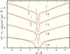 |
Fig. 2 Comparison of STIS and FUSE observations around H i L α–δ with our final model. Thick (red in the online version) photospheric + ISM line absorption model with NH i = 2.2 × 1018 cm-2; thin (blue) pure photospheric model; dashed (green, L α only) NH i = 1.2 × 1018 cm-2, 3.2 × 1018 cm-2. The locations of the D i blends are marked. L β–δ are shifted in flux (0.7, 1.6, 2.7 × 10⁻¹¹ erg cm-2 s-1 Å-1) for clarity. A reddening of EB − V = 0.0005 is applied following the law of Fitzpatrick (1999, with RV = 3.1. |
Besides H i and D i, we identified interstellar lines of C ii– iv, N i– ii, O i, Al ii, Si ii– iii, P i– ii, S i– ii, and Fe ii in the FUSE and STIS spectra (Table 5). To identify pure photospheric lines that are contaminated by ISM lines, we modeled all of these and found that we need two distinct clouds with vrad = 9 ± 1 km s-1 and vrad = 19 ± 1 km s-1. This is well in agreement with the measurements of Sahu et al. (8.6 ± 1.7 km s-1 and 19.3 ± 2.5 km s-1 1999), who assigned the latter value to the local interstellar cloud. Dickinson et al. (2012b) measured 8.5 ± 0.18 km s-1 and 19.3 ± 0.03 km s-1. They unambiguously detected that the first cloud is of circumstellar origin. An additional third cloud with intermediate velocity like assumed by Vidal-Madjar et al. (1998, vrad = 8.2,13.2,20.3 ( ± 0.8 km s-1 is not necessary for our modeling (Fig. 3, top).
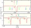 |
Fig. 3 STIS spectrum around the interstellar absorption lines O iλ 1302.163 Å (top) and N iλλ 1199.550,1200.223,1200.710 Å (bottom) compared with the synthetic spectrum of our final model where the ISM lines are included. The labels give the radial velocities (in km s-1) that are applied. |
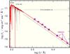 |
Fig. 4 Comparison of FUSE and HST (STIS and NICMOS) observations with our final model. A reddening of EB − V = 0.0005 is applied. The low-resolution (LR) STIS+NICMOS observation vanishes behind the model SED due to the line width. Therefore, we plotted the observed spectrum twice, one shifted by Δlog fλ = −0.2 for clarity. U,R,I (Landolt & Uomoto 2007), B,V (Høg et al. 2000), J,H, and K (Cutri et al. 2003) fluxes (converted from brightnesses using values given by Heber et al. 2002) are shown for comparison. |
Interestingly, we find additional weak absorptions of O I λ 1302.163 Å and N I λ 1199.550,1200.223,1200.710 Å at vrad of − 26.3 km s-1 and − 26.1,km s-1, respectively. These velocities are reminiscent of the expansion velocity of a planetary nebula shell (e.g.. Kwok et al. 1978), that for a stellar mass of M = 0.555 M⊙ (Sect. 4.6) must have been ejected more than 500 000 years ago (Renedo et al. 2010). Its recombined, neutral gas, however, is still in the line of sight.
From the low interstellar NH i density, we expect a low interstellar reddening. The Galactic reddening law of Groenewegen & Lamers (1989), log (NH i/EB − V) = 21.58 ± 0.10, predicts 0.0003 ≲ EB − V ≲ 0.0007. Figure 4 shows a comparison of observations and synthetic spectrum from the far UV (FUV) to the IR. We find EB − V = 0.0005 ± 0.0005.
3. Model atmospheres and atomic data
Table 2 demonstrates clearly that a panchromatic analysis from the EUV to the optical is inevitable for accurate results on photospheric parameters. Moreover, NLTE modeling is mandatory to calculate a reliable synthetic spectrum.
Lanz et al. (1996) presented the first NLTE model (Table 2) that reproduced the observed spectrum from the EUV to the optical wavelength range. Barstow & Hubeny (1998) introduced then a stratified H+He envelope including heavier metals in their models to improve the match to the observed flux below the He ii absorption threshold (λ ≲ 228 Å). Later analyses had shown that there is further evidence for a stratification in G191−B2B’s photosphere. Vennes et al. (2000) closely examined Feige 24 that, compared with G191−B2B, has similar atmospheric parameters and an almost identical abundance pattern. They found that the O iv / O v ionization equilibrium is overcorrected by − 0.8 dex in their NLTE model. They concluded that this might reveal an inhomogeneous vertical stratification of oxygen in both stars. A later analysis of both stars (Vennes & Lanz 2001) showed that the average heavy-metal abundance in Feige 24 is 0.17 dex larger compared to the cooler and, hence, older G191−B2B (same log g). Thus, the abundance pattern is determined by the same processes in both stars and the authors assumed that selective radiative pressure and gravity are in diffusive equilibrium. This was proven by Dreizler & Wolff (1999). They used self-consistent diffusion models (Table 2) that were able to reproduce the observed flux for λ ≲ 228 Å without additional absorbers or mechanisms. However, problems remained with the fit to the UV lines.
Now, our strategy to proceed with the analysis is threefold. We start with chemically homogeneous models to find the model that reproduces best the continuum slope and the spectral lines from the FUV to the optical (Sect. 4). In an intermediate step, we will then apply the depth-dependent abundance profiles calculated by Dreizler & Wolff (1999) to our final homogeneous model to investigate the impact of chemical stratification on the emergent spectrum (Sect. 4.3). In the last step, a diffusion model is calculated and compared with the homogeneous model (Sect. 4.4).
4. Spectral analysis and results
The metal-line blanketed NLTE model atmospheres for our analysis were calculated with the state-of-the-art Tübingen NLTE model-atmosphere package (TMAP6, Werner et al. 2003), which can consider opacities of all elements from H to Ni and beyond (Rauch 1997, 2003; Werner et al. 2012; Rauch et al. 2012). TMAP was successfully used for the spectral analysis of hot, compact stars (e.g. Rauch et al. 2007; Wassermann et al. 2010; Ziegler et al. 2012).
Our models assume plane-parallel geometry and are in hydrostatic and radiative equilibrium. Opacities of all species for which spectral lines are identified, namely H, He, C, N, O, Al, Si, P, S, Ca, Sc, Ti, V, Cr, Mn Fe, Co, Ni, Zn, Ge, and Sn, were considered in the model-atmosphere calculations. For all elements, we account for level dissolution (pressure ionization) following Hummer & Mihalas (1988) and Hubeny et al. (1994). Figure 5 demonstrates that our H i model ion (Table 4) includes all levels that are relevant in the line-forming region −4.5 < log [m/(g/cm2)]. All model atmospheres presented here cover column densities m of − 7.6 < log m < 3.2 (cf. Beuermann et al. 2006) represented by 90 depth points.
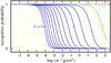 |
Fig. 5 Occupation probabilities of the H i levels with principal quantum numbers n = 1 − 14 in our final model. |
The model-atoms and respective absorption cross-sections for Ca–Ni were calculated via the recently registered VO service TIRO7 that uses Kurucz’s atomic data8 and line lists (Kurucz 1991, 2009, 2011).
Ca, Sc, Ti, V, Cr, Mn, and Co lines are not identified. These were merged into a generic model atom (Rauch & Deetjen 2003) with fixed solar abundance ratios. Then, we performed test calculations and adjusted the abundance to a value (1.78 × 10⁻⁶ by mass, the solar value is 9.93 × 10⁻⁵) where all of its lines just fade in the noise of the observed spectra. All other model atoms were constructed from data retrieved from the public Tübingen model-atom database TMAD9.
In total, we considered 1038 atomic levels in NLTE combined with 4646 line transitions (for the number of individual iron-group lines, see Table 4) in the model-atmosphere calculations with 53 203 frequency points within 1 × 10¹² Hz ≤ ν ≤ 3 × 10¹⁷ Hz. For the emergent spectra (100 Å ≤ λ ≤ 400 000 Å, 686 196 wavelength points), we account for fine-structure splitting and used 1585 NLTE levels and 9721 respective line transitions. The model-atom statistics are summarized in Table 4. Figure 6 shows the ionization fractions of all elements in our final model. It may be interesting to note that a single model atmosphere needs about one week to converge, i.e. the absolute values of all relative corrections are below 10-4, on a 64 bit, 2.66 GHz compute core with 8 GB memory.
For the calculation of synthetic H i line profiles, we use Stark line-broadening tables provided by Tremblay & Bergeron (2009). For those lines, where no broadening tables are available, TMAP uses an approximate formula, as described in Ziegler et al. (2012, Eqs. (1)–(5)).
We started with a model with and log g = 7.55 (the values of Gianninas et al. 2011) and the element abundances from Table 3. Next, we adjusted these abundances to best reproduce the respective spectral lines. We then calculated an extended grid of 234 model atmospheres (48 000 K ≤ Teff ≤ 68 000 K in steps of ≤1000 K and 7.35 ≤ log g ≤ 7.75 in steps of 0.05 (some of the hotter models are calculated only for log g ≤ 7.60). For this grid, we extensively used compute resources of the bwGRiD10 in addition. Although this highly speeded up the model-grid calculation, the wide parameter range and the large number (15) of parameters to adjust simultaneously did not allow us to take a statistical approach in the spectral analysis (χ2 method like e.g. in Gianninas et al. 2011) on a reasonable time scale. We therefore need to rely upon our “χ-by-eye” methods. All SEDs that were calculated for this analysis are available via TheoSSA11.
In a first analysis step, we will determine log g based on UV and optical observations. Then, we will determine Teff precisely based on ionization equilibria of the metals which are sensitive indicators. Subsequently, we will adjust the abundances again and verify our Teff and log g results.
4.1. Surface gravity and effective temperature
The dependency of the synthetic flux level on Teff and log g for fixed abundances is demonstrated in Fig. 7, where we compare the observed and synthetic fluxes in the FUV. In the top panel, it is obvious that at a constant , a log g higher by 0.2 dex than log g = 7.55 measured by Gianninas et al. (2011) is necessary to reproduce the Lyman-line decrement. For a fixed log g = 7.55 (middle panel), a lower Teff (Δ Teff = 6000 K) improves the agreement between model and observation. The bottom panel shows that at values within the (statistical) error ranges from the H i Balmer-line analysis, and log g = 7.60 (cf. Table 2Gianninas et al. 2011), a good agreement for both, line profiles and decrement, is achieved.
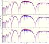 |
Fig. 7 Section of the FUSE observation compared with our model fluxes with different Teff and log g. In the top and middle panels, the synthetic fluxes are normalized to the observed flux at 1000 Å and in the bottom panel to the observed K magnitude (see Fig. 4). EB − V and NH i are applied using our results from Sect. 2.3. |
This was not expected from the outset although Barstow et al. (1998) found a relatively good agreement of Teff and log g from H i Lyman and Balmer lines in the heavy-metal rich models (Table 2). The later analysis by Barstow et al. (2001, Table 2 shows strong deviations in log g between optical and FUV analyses. Figure 8 shows a comparison of synthetic H i Balmer line profiles with optical observations. The deviation between the / log g = 7.55 and the 60 000/7.60 ones is minor.
In addition to the low-resolution (R ≈ 500) optical spectrum, medium-resolution (R ≈ 6000) observations of Hα and Hβ are shown is Fig. 9. The agreement among the STIS low and medium resolution is excellent. While the model absorption is a bit weak as shown in the lower plot of Fig. 9, the central NLTE emission reversal agrees well with the observations.
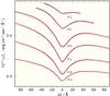 |
Fig. 8 Synthetic H i Balmer-line profiles compared with the STIS LR observation. The observation is shifted by factors of 0.921, 0.323, 0.232, 0.202, 0.193, and 0.188 for Hα – Hζ, respectively, to fit into this plot. Red, full line: and log g = 7.60; blue, dashed: and log g = 7.55. |
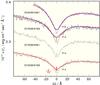 |
Fig. 9 STIS Hα and Hβ low-resolution (dashed, blue) and medium-resolution (gray lines) observations (labeled with medium-resolution grating/central wavelength in Å). Because of uncertainty in the flux calibration, the medium-resolution data are normalized to the low-resolution flux. The flux around Hβ in the top plot is multiplied by a factor of 0.35. The red lines in the upper two plots are the medium-resolution (R ≈ 6000) spectra degraded to the low resolution (R ≈ 500) and agree with the low resolution (blue dash) within the uncertainty of the R = 500 resolution. The lower two plots are shifted down by 0.035 and 0.07 × 10⁻¹³ flux units, respectively. In the lowest plot, the model is overplotted in red after smoothing to the medium resolution. While the model Hα absorption is somewhat too weak, the central emission agrees with the observation within the uncertainty of the resolution (insert). |
Although we cannot reproduce Hα and Hβ in detail in the medium-resolution spectrum, this has no significant influence on our determination of Teff and log g because the higher members of the H i Balmer series form much deeper in the atmosphere where the influence of metal opacities is less important (cf. Napiwotzki & Rauch 1994). We adopt log g = 7.60.
In the next step of this analysis, we evaluate ionization equilibria of metals that exhibit lines of successive ionization stages. Figures 10–12 show some strategic lines for this Teff determination. In total, we can use eight elements and lines of C iii– iv, N iii– v, Si iii– iv, P iv– v, S iv– v, Fe iv– vi, Ni iv– vi, and Ge iv– v. reproduces well all these equilibria simultaneously. For our further analysis, we adopt .
4.2. Photospheric abundances
In the following, we use logarithmic mass fractions for all abundance values, if not otherwise mentioned. Previously determined abundances and respective references are summarized in Table 3. In the following, we will briefly mention the strategic lines for the abundance determinations and note abnormalities for an element selection only. Most of the identified metals exhibit lines of at least two subsequent ionization stages and some of these lines were already used for the determination of Teff (Sect. 4.1). The abundances were then adjusted to achieve best line fits. Two large plots (Figs. A.1, A.2, German DIN A0 size) are provided in the online material that show a comparison of our final model with the observation in the FUSE and STIS wavelength ranges (in total 911 − 1750 Å). They include all line identifications (FUSE/STIS wavelength range), e.g. 2/421 Fe iv, 144/815 Fe v, 1/52 Fe vi, 1/236 Ni iv, 13/690 Ni v, and 9/43 Ni vi lines. These numbers are much higher than those of Preval et al. (2013, 106 Fe v and 44 Ni v . The recent work of Berengut et al. (2013) to employ G191−B2B as a stellar laboratory to determine the fine-structure constant is based on the latter list and may, thus, not fully exploit capacity of all the available STIS spectra of G191−B2B.
Our line identifications are also summarized in Table 5, whereas Table 6 gives a list of the strongest unidentified lines.
4.2.1. Helium
The first analyses revealed only upper limits for the He abundance, e.g. He < − 3.1 and <4.1 (Vennes et al. 1996; Gunderson et al. 2001, respectively). Cruddace et al. (2002) determined He = −4.2 ± 0.1 using high-resolution EUV spectroscopy. An attempt to identify and measure He ii Lyman lines (n − n′ = 1–4, 1–5) with J-PEX12 (Barstow et al. 2005) was not successful. Our models show that He II λ 1640 Å (2–3) should be clearly visible at He = −3.7 and − 4.2 and disappears in the noise of the observation only at about He < − 4.7 (Fig. 13). We adopt this upper-limit value for our models.
Wavelengths (in Å) of unidentified strong (Wλ > 10 mÅ), likely photospheric lines in the FUSE and STIS observations.
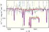 |
Fig. 13 Synthetic spectrum around He iiλ 1640.42 Å compared with the STIS observation. He abundances are green, dashed: −10.0, red, thick: −4.7, blue, thin: −4.2, blue, dashed: −3.1. The insert shows the region Δλ = ± 0.4 Å around the He ii line. For comparison, the observation was smoothed with a low-pass filter (Savitzky & Golay 1964, n = 15, m = 4). |
4.2.2. Carbon, nitrogen, and oxygen
C iii and C iv lines are visible in the observation. C III λ 977.02 Å and C IV λλ 1548.20,1550.77 Å have strong ISM blends. In case of the latter, the photospheric component can be separated and modeled (Fig. 10). At C = −5.15, lines of both ions are well reproduced.
N iii– v lines are found in the observation, they are all well matched at N = −5.58 (Fig. 10).
Vennes et al. (2000) encountered deviations between oxygen abundances determined from O iv and O v lines in an analysis of Feige 24. The O v abundance was 0.5 dex higher in their LTE model approach. In their NLTE models, they found that the O iv / O v ionization equilibrium was overcorrected by − 0.8 dex. They suggested an inhomogeneous stratification of O in the atmosphere. Vennes & Lanz (2001) discovered that a similar problem exists in G191−B2B, with an overcorrection of − 0.6 dex. Consequently they assumed that in both stars, the interplay between selective radiation pressure and gravity in diffusive equilibrium are the key processes for this phenomenon. Figure 14 shows the same deviation in our models. While O IV λλ 1338.615,1342.990,1343.526 Å are well fitted at O = −4.72, O V λ 1371.296 Å is apparently much stronger than observed. It is matched with an O abundance that is reduced by − 0.4 dex.
In the FUSE observation, only the short wavelength component of the O VI λλ 1031.912,1037.614 Å resonance doublet is detectable. The unexpected weakness of this doublet was already reported by Oegerle et al. (2005). Dickinson et al. (2012b) verified that it stems from the photosphere. The O vi resonance doublet in our models is even stronger, compared to O iv and O v lines, requiring a reduction of the O abundance by about –1.5 dex (Fig. 14). Dickinson et al. (2012a) encountered a similar problem with enigmatically deep line profiles of the N v resonance doublet in their models. We revisit the problem with the oxygen abundances derived from different ionization stages in Sects. 4.3 and 4.4 in detail.
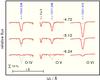 |
Fig. 14 Most prominent O iv, O v, and O vi lines in the STIS and FUSE observations compared with our theoretical line profiles calculated with three O abundances (O = −4.72, –5.12, –6.24, from top to bottom). |
4.2.3. Aluminum, silicon, phosphorus, and sulfur
Holberg et al. (1998) identified the Al III λλ 1854.72,1862.79 Å resonance doublet in the IUE NEWSIPS SWP Echelle Data Set13, and Holberg et al. (2003) measured Al = −5.08. We could newly identify some other Al iii lines. We derive Al = −4.95, well in agreement with the Holberg et al. (2003) value (Fig. 15).
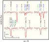 |
Fig. 15 Theoretical Al iii line profiles calculated from our final model compared with the STIS observation. |
Si iii– iv, P iv– v, and S v– vi lines are identified. We determine Si = −4.30, P = −5.81, and S = −5.24 (Fig. 10).
4.2.4. Iron-group elements
Many hundreds of lines of Fe iv– vi and Ni iv–vi are identified (Table 5). They are best reproduced at Fe = −3.30 and Ni = −4.45. Note that the Ni/Fe abundance ratio is about 25% higher than the solar ratio. Some of these lines are shown in various figures in this paper, please have a look at the two large online figures that show the complete FUSE and STIS wavelength ranges. An animation of STIS wavelength range can been seen at http://astro.uni-tuebingen.de/~rauch/A0_E140H_SW.gif as well.
In Fig. 15 three lines of Cr iv and one of Co iv are visible in the synthetic spectrum of our final model. These are weak and comparable to the noise of the observation. Although one may be tempted to believe the presence of Cr IV λ 1863.075 Å, we take this as a hint that a log mass fraction of − 5.75 for the generic model atom is reasonable and adopt this as an upper limit for our analysis. This is, within the error limits, in agreement with the upper limits for Cr, Mn, and Co of about − 6.2 that were found by Holberg et al. (2003).
Preval et al. (2013) suggested that the unidentified line at 1272.98 Å is a V iv line. Since many other V iv lines with much stronger log gf values (g is the statistical weight of the lower atomic level and f is the oscillator strength of the line transition) from Kurucz’s POS line lists (with good wavelengths) are not present in the spectrum, e.g. V IV λλ 1355.127,1419.577,1426.647 Å (all more than ten times higher log gf) therefore this identification appears to be very unlikely.
We mention here that we find deviations between Kurucz’s POS wavelengths and the observation of up to 0.05 Å. In addition, Fig. 13 shows that the strengths of Fe IV λ 1640.042 Å and Fe IV λ 1640.155 Å in the model are the opposite way around in the observation.
Figure 16 shows a comparison of models (calculated with Kurucz’s POS lines) in the FUSE and STIS wavelength ranges where in each case the abundance of an individual element X in the construction of the generic (Ca, Sc, Ti, V, Cr, Mn, Co) model atom is increased by a factor of ten. Values higher that 1 in the flux ratio indicate stronger lines of element X.
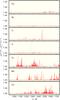 |
Fig. 16 Flux ratio of our final model and a model with ten times increased abundance of element X (Ca to Co, from top to bottom). The location of V ivλ1272.98 Å is marked. |
E.g. the case of Ti, two lines are much stronger than all others, Ti IV λλ 1451.739,1467.343 Å. They are not identified in the observation but at the ten times increased abundance they are clearly visible in the model. The same is valid for Cr, where Cr IV λλ 1332.415 Å and Cr VI λλ 1417.660 Å are the strongest lines in our models (Fig. 16), and for Mn and Co as well. This allows us to establish upper abundance limits of about 10% solar for Ti, Cr, Mn, and Co (cf. the beginning of Sect. 4).
4.2.5. Zinc, germanium, and tin
21 Zn iv lines are newly identified in the STIS observation. These are almost all that are listed in the NIST14 database with relative intensities higher than 100. Since no individual calculations for Zn iv transition probabilities are available, we adapted those of the isoelectronic Ge vi (Rauch et al. 2012). In Fig. 17, we show nine of them with NIST relative intensities of 200. All their theoretical line profiles are reproduced at Zn = −4.89.
For Ge, we used the same model atom as Rauch et al. (2012) and determined Ge = −5.49 (Fig. 10).
We constructed a relatively small Sn model atom. The only lines for which reliable oscillator strengths are available are the Sn iii and Sn iv resonance lines (Morton 2000). For all other allowed transitions, we follow Werner et al. (2012) and set f = 1. We used the Sn IV λ 1314.537 Å resonance line, like Vennes et al. (2005), to measure the abundance of Sn = −6.45.
4.2.6. Summary of results with chemically homogeneous models
We can reproduce the entire ultraviolet spectrum of G191−B2B with our chemically homogeneous NLTE models, with the exception of the O iv/ vi lines which are obviously affected by O stratification effects. Current diffusion models yield poor fits to the metal lines (Dreizler & Wolff 1999). and log g = 7.60 ± 0.05 were determined within small error limits. They are in agreement with Gianninas et al. (2011, Teff = 60 920, log g = 7.55 ± 0.05). We do not encounter problems in modeling H i Lyman and Balmer lines simultaneously with the same Teff and log g like found by Barstow et al. (2001, see Table 2.
We can determine all abundances with error limits of 0.2 dex. In case of Zn, where we adopt Ge vi f-values, we estimate that the error is 0.3 dex. Our C, N, O, Al, Si, Fe, and Ni abundances (Fig. 18) agree, within error limits, with those of Vennes et al. (1996); Holberg et al. (2003); Vennes et al. (2005). Our values are in general slightly higher. One reason may be the about 6000 K higher Teff of our final model. The stellar parameters are summarized in Table 8.
The abundances of all elements but Fe predicted by Chayer et al. (1995) for a DA-type WD differ strongly from those that we determined (Fig. 18).
4.3. Test of the diffusion impact
In a first step, we simply applied the abundance profiles provided by Dreizler & Wolff (1999) to the occupation numbers of He, C, N, O, Si, and Ni in our final model. Figure 19 (top panel) shows that this gives a good agreement with O v while O iv is now too weak. The O vi lines appears even stronger, strengthening the discrepancy. Since the atmospheric structure was kept fixed in this test, we expected that, if at all, only a self-consistent diffusion model is able to reproduce the observed O iv– vi lines simultaneously.
4.4. A self-consistent diffusion model
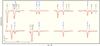 |
Fig. 17 Theoretical line profiles of the strongest Zn iv lines in the STIS wavelength range compared with the observation. |
We used the NGRT15 code (Dreizler & Wolff 1999; Schuh et al. 2002) to calculate diffusion models with the same element composition and model atoms like our homogeneous TMAP models. The first model shows a strongly increased abundance of the generic model atom that combines Ca, Sc, Ti, V, Cr, Mn, and Co (Sect. 4) and, hence, much too strong lines of the considered elements. The reason is that the IrOnIc code (Rauch & Deetjen 2003) calculates a mean atomic weight for the generic atom following  (1)where ri is the relative mass-fraction (with respect to r1 = 1) and Ai the atomic weight of element i. The artificially increased number of lines of a single generic element strongly increases its radiative levitation. Flux blocking by the generic element then leads to stronger gravitational settling of other elements, e.g. Sn had an abundance below 10-17 throughout the model atmosphere. The other elements showed abundances that were partly more than one dex below those of our homogeneous model. Since we did not want to neglect all opacities of the generic atom, we changed its atomic weight to
  (2)Now, the stratified NGRT models yields depth dependent abundances (Fig. 20) that are closer to those of our homogeneous model, especially Sn appears at a realistic value. In case of He, C, N, O, Si, and Ni the abundance profiles are similar to those of (Dreizler & Wolff 1999). The changed atmospheric structure is shown in Fig. 21. It is interesting to note that most of the lines and all continua are formed at log m ≳ − 3 (Fig. 22) while deviations in the temperature structure are noticeable only outside of this region. The resulting spectrum (Fig. 23) of the stratified model is, compared with the homogeneous model, no improvement. While Fe v lines match the observation at about , it can be extrapolated that Fe iv lines are much too strong for Teff ≲ 70 000 K. Ni iv and Ni v lines are much too strong because the Ni abundance is enhanced (Fig. 20) in the line-forming regions and can, thus, not be used for a Teff estimate.
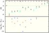 |
Fig. 18 Top: photospheric abundances of G191−B2B (red stars) compared with solar values (Asplund et al. 2009). [X] denotes log (mass fraction/solar mass fraction) of element X. The dashed, green line shows the solar ratio. The arrows indicate upper limits. The cyan diamonds (Holberg et al. 2003), triangles (Vennes et al. 1996), and tridents (Vennes et al. 2005) are previously determined values. Bottom: comparison of our abundance number ratios (red stars) with predictions of diffusion calculations for DA-type (blue squares) WDs (Chayer et al. 1995) with and log g = 7.5. |
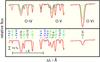 |
Fig. 19 Same as Fig. 14. Top: dashed, green TMAP (=chemically homogeneous) model with O = −4.72; thin, blue TMAP model with abundance profiles from Dreizler & Wolff (1999), thick, red NGRT (=diffusion) model. Bottom: thick, red NGRT model with an artificially reduced O abundance in the outer atmosphere. Note that in the NGRT models, the line strengths of the generic iron-group element (see text) are overestimated. |
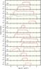 |
Fig. 20 Abundance profiles in our diffusion model (, log g = 7.60). Short-dashed (blue) lines: unrealistically high abundance of the generic iron-group element (IG, see text), thick (red) lines: reduced IG abundance, horizontal long-dashed, thin (cyan) lines: the abundances in our final homogeneous model. In the O panel, the thick dashed (green) line shows our modified O-abundance profile (see text). |
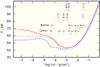 |
Fig. 21 Temperature structures (, log g = 7.60) of a pure H model (thin, black), our final homogeneous model (thick, red), and a diffusion model (dashed, blue). The formation depths of the line cores of the lowest members of the H i Lyman and Balmer series, the C iv, N v, O vi, Si iv, and S vi resonance doublets, and our strategic O ivλλ 1338.634,1343.022,1343.526 Å and O vλ 1371.296 Å lines are marked. |
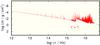 |
Fig. 22 Optical depth τ = 1 in our final homogeneous model. |
In the stratified models, the O iv and O v lines are now mucher stronger than observed and O vi appears at the same strength that resulted from our diffusion test (Sect. 4.3). The O abundance profile (Fig. 20) shows a strong increase for log m < − 4. Only by the introduction of an artificial abundance reduction by a factor of m/1585 for log m ≲ − 3.2, we achieve an acceptable agreement of O v and O vi (Fig. 19). O iv is still slightly too strong because the abundance and, thus, the lines (including a blend at O iv) of the generic iron-group atom (Sect. 3) are overestimated by the NGRT model (Fig. 20). Based on this numerical exercise, it may be speculated that a weak stellar wind or an other, unknown process that is not considered by NGRT is responsible for the lower oxygen abundances in the outer atmosphere.
We can conclude two things. A generic model atom is obviously not suited for a diffusion calculation due to the strongly enhanced number of lines for a single atom in the modeling process. The NGRT diffusion models yield partly too low abundances in the line-forming regions and, thus, cannot reproduce the metal line properly. An additional, weak wind may be necessary to increase the metal abundances in the line-forming regions.
4.5. The extreme-ultraviolet spectrum
The inability to model the EUVE spectrum with chemically homogeneous atmospheres (Holberg et al. 1989) was the reason to investigate stratified photospheres (e.g. Koester 1991). Lanz et al. (1996) demonstrated, that it is possible to consistently match the optical, UV, and EUV data with homogeneous NLTE models with the same Teff and chemical composition.
We calculated EUV spectra from our model grid with 193 584 frequency points within 100 Å ≤ λ ≤ 930 Å, and Kurucz’s LIN line lists (theoretical and laboratory measured lines, in total 8 135 405 lines of Ca–Ni in our wavelength interval, Kurucz 2009). These spectra were processed with the recently registered VO tool TEUV16 that corrects synthetic stellar fluxes for interstellar absorption below 911 Å. It simulates radiative bound-free absorption of the lowest ionization states of H, He, C, N, and O using Opacity Project data (Seaton et al. 1994). Two interstellar components with different radial and turbulent velocities, temperatures, and column densities can be considered. Figure 24 shows the comparison of synthetic and observed EUV spectra. Our synthetic spectra were normalized to the measured FUSE flux of 1.347 × 10⁻¹¹erg cm-2 s-1 Å-1 at 920 Å. Then, the interstellar column densities are adjusted, to match the EUVE flux NH i for 530 Å, NHe i for 470 Å, and NHe ii for 220 Å. Since our models do not reproduce the measured flux between 250 Å and the He ii ground state threshold, NHe ii is not reliable. Table 7 shows the applied NH i and NHe i values compared with the literature values. Our NH i values, necessary to match the EUVE flux level, are about a factor of two higher than 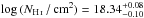 that we determined previously from H i Lyman-line fits (Sect. 2.3). log NN i = 13.87 and log NO i = 14.86 were adopted from Lemoine et al. (2002).
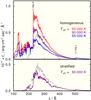 |
Fig. 24 Top: comparison of three synthetic spectra (Teff = 55 000, 60 000, and 65 000 K) of chemically homogeneous models with the EUVE observation. The wavelengths of ground-state absorption thresholds of He ions are indicated. Bottom: comparison of a stratified model with the observation. |
The overall agreement of our homogeneous models with at wavelengths λ ≳ 250 Å is very good, especially the interval 360 Å ≲ λ ≲ 450 Å is excellently matched in detail. Models with and yield much too high and too low fluxes, respectively. At λ ≲ 250 Å the theoretical flux is too high in all models, even at . A stratified model (Fig. 24) with fails to reproduce the flux between 250 Å ≲ λ ≲ 420 Å and has a too-high flux at λ ≲ 200 Å.
Both, our homogeneous and our stratified models, fail to reproduce the entire EUV spectrum of G191−B2B. It seems likely that there may be some stratification in the atmosphere but we don’t yet know how to distribute the various atomic species with depth. This is a challenge for theorists.
4.6. Mass and distance
A stellar mass of  and a luminosity of
  are determined by comparison with evolutionary models (Fig. 25) for old white dwarfs (metallicity z = 0.001).
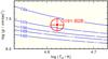 |
Fig. 25 Location of G191−B2B in the log Teff–log g plane (the ellipse indicates the errors of our analysis) compared with evolutionary tracks for hydrogen-rich white dwarfs (Renedo et al. 2010) labeled with the respective stellar masses (in M⊙). |
We calculated the spectroscopic distance following the flux calibration of Heber et al. (1984b) for λeff = 5454 Å, ![\begin{eqnarray} d[\mathrm{pc}]=7.11 \times 10^{-4} \cdot \sqrt{H_\nu\cdot M \times 10^{0.4\, m_{\mathrm{v}_0}-\log g}}, \end{eqnarray}](/articles/aa/full_html/2013/12/aa22336-13/aa22336-13-eq259.png) (3)with mVo = mV − 2.175c, c = 1.47EB − V, and the Eddington flux Hν = 1.109 × 10⁻³ erg cm-2 s-1 Hz-1 at λeff of our final model atmosphere. We used EB − V = 0.0005 ± 0.0005 (Sect. 2.3), , and mV = 11.7228 ± 0.0082 (van Leeuwen 2007), and derived a distance of d = 62 ± 4 pc and a height above the Galactic plane of z = 8 ± 1 pc. This is in agreement with the Hipparcos17 parallax measurement (van Leeuwen 2007, HIP23692) of
(3)with mVo = mV − 2.175c, c = 1.47EB − V, and the Eddington flux Hν = 1.109 × 10⁻³ erg cm-2 s-1 Hz-1 at λeff of our final model atmosphere. We used EB − V = 0.0005 ± 0.0005 (Sect. 2.3), , and mV = 11.7228 ± 0.0082 (van Leeuwen 2007), and derived a distance of d = 62 ± 4 pc and a height above the Galactic plane of z = 8 ± 1 pc. This is in agreement with the Hipparcos17 parallax measurement (van Leeuwen 2007, HIP23692) of  pc and the XHIP18 value of d = 57.96 ± 10.31 pc (Anderson & Francis 2012). The spectroscopic distance of d = 55.84 ± 0.86 pc determined by Holberg et al. (2008) is slightly smaller, this error estimate, however, appears to be too optimistic.
5. TheoSSA: synthetic stellar spectra on demand
At the end, we want to compare our final TMAP model flux with an SED, that was calculated with the TMAW tool (Sect. 1) and considers H, He, C, N, and O only. Figure 26 shows that the TMAP flux is higher everywhere at λ > 911 Å. The reason is strong metal-line blanketing at λ < 911 Å that causes a flux increase at longer wavelengths. It amounts to about 10% at 1000 Å and to about 5% at 7000 Å. The lower panel of Fig. 26 illustrates that the theoretical line profiles of the H i Balmer series are almost identical in both, TMAP and TMAW models, with the exception of an increased emission reversal in the line core of Hα in the TMAP model.
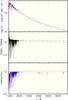 |
Fig. 26 Comparison of our final TMAP model (blue, thick) with a TMAW model (red, thin). Top: astrophysical fluxes at the stellar surface, middle: ratio TMAP/TMAW flux, bottom: normalized fluxes. |
The TheoSSA database contains currently TMAP SEDs of a dozen standard stars. Some of them are represented by different models for comparison, because they were initially calculated for the calibration (Vernet et al. 2008a,b, 2010) of ESO’s19 second generation VLT20 instrument XSHOOTER21 (Vernet et al. 2011) while the parameters of Gianninas et al. (2011) and Giammichele et al. (2012) were published later (Table 9).
Standard star SEDs (references for Teff and log g are given) presently available in TheoSSA.
6. Accuracy of flux calibration with G191−B2B
Our spectral analysis was performed using state-of-the-art atomic data and model-atmosphere code. The best reproduction of UV and optical spectra was achieved with chemically homogeneous models. In Fig. 27, we compared two models at the edge of our error ranges in Teff and log g. The deviation in the continuum flux of two TMAP model SEDs is ≈3% in the optical and ≈5% in the FUV. A systematic error is present due to the uncertainty of the used atomic data, such as oscillator strengths where it is typically ≈15% for a single line. The employment of many lines of many ions of many atoms in a spectral analysis minimizes the propagation of these uncertainties into the errors of the main photospheric properties like Teff, log g, and the abundances. An additional systematic error may be present between individual model-atmosphere packages (e.g. Rauch 2008b) because of differences in coding, approximations, etc.
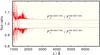 |
Fig. 27 Flux ratio of two TMAP models at the edge of the Teff and log g error ranges and our final model. |
The situation for the flux calibration is, however, not that strongly dependent on the exact Teff and log g values (the latter is even less important). E.g. in the case of G191−B2B and our errors (3% in Teff and 0.05 dex in log g), a normalization to a precisely measured brightness will reduce the deviation between model SED and observation much below 1% in the optical and infrared. The residuals among the three primary stars G191−B2B, GD 71, and GD 153 are generally sub percent at the longer wavelengths (Bohlin 2007). The remaining deviation in the FUV wavelength range is presently less than 2%. Further improvement is essentially dependent on the reliability of the atomic data (Sect. 7).
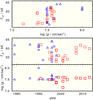 |
Fig. 28 Determined Teff and log g values in the last 34 years. Blue triangles denote analyses with LTE models, red squares those with NLTE models (Table 2). The result of Koester et al. (1979, log g = 5.95 is outside the top and bottom panels. |
7. Conclusions
The TheoSSA service is designed to provide theoretical stellar SEDs of any kind in VO-compliant form. Its efficiency is strongly increasing if more different model-atmosphere groups provide their SEDs with a proper description in their respective meta data. The establishment of a database of spectrophotometric standard stars is an opportunity to use the same model SEDs for astrophysical flux calibration. Many model-atmosphere groups have their own best models for some of these stars, for which a common base for comparison arises. Differences in the algorithms for considered physics, assumptions, and approximations in different model-atmosphere codes, lead to systematic deviations in general.
Figure 28 shows the temporal development of the Teff and log g determinations of G191−B2B. While both values had a large scatter in the 1990s (error ranges are not shown for clarity), the three most recent analyses, that are all based on sophisticated NLTE model-atmosphere techniques, show a good agreement within relatively narrow error ranges of about 3% in Teff and 0.05 dex (≈12%) in log g. Ironically, these latest results agree quite well with the very first line-profile analysis presented by Holberg et al. (1986) performed with a Ly α line-profile fit with a simple, pure-H LTE model atmosphere. The TheoSSA database may help to get closer to the intended goal of 1% accuracy in absolute flux calibration.
We presented here our spectral analysis of G191−B2B to demonstrate the current state-of-the-art. We are presently able to reproduce the observed spectrum from 250 Å to the infrared. The EUV part from 150 Å to 250 Å cannot be modeled, neither by our homogeneous nor by our stratified models. The reason is unknown.
A similar analysis of the UV spectrum of the calibration star BD + 28°4211 (,  ) was just published by Latour et al. (2013).
Model-atmosphere codes have arrived now at a high level of sophistication, and we already encounter problems getting reliable atomic data to reproduce the high-resolution and high-S/N spectra that are obtained with presently available instruments. This is a challenge for atomic physicists to be prepared for upcoming telescopes and instruments.
Online material
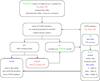 |
Fig. 1 Flow diagram of TheoSSA. The VO user sends an SED request to the GAVO database by entering the photospheric parameters. If a suitable model is available within the desired tolerance limits, it is offered as a results table. In case that the parameters are not exactly matched, the VO user may decide to calculate a model with the exact parameters. TMAW will start a model-atmosphere calculation at our institute’s (IAAT) PC cluster then. Extended model grids make use of computer resources that are provided by AstroGrid-D. As soon as the model is converged, the VO user can retrieve the SED table from the GAVO database. |
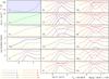 |
Fig. 6 Temperature and density structure and ionizations fractions of our model with and log g = 7.60. IG denotes a generic model atom consisting of Ca, Sc, Ti, V, Cr, Mn, and Co. |
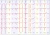 |
Fig. 10 Synthetic line profiles of C iii– iv, N iii– v, Si iii– iv, P iv– v, S iv– v, and Ge iv– v calculated from models with 57 000 K ≤ Teff ≤ 62 000 K and log g = 7.6 compared with FUSE and STIS observations. The small horizontal bars, labeled with the element’s name, indicate Teff where the ionization balance is best reproduced. The lines are identified at the top. “is” denotes interstellar origin. In the cases of C iv λλ 1548,1550 Å, C iv λλ 1548,1550 Å, and Si iii λλ 1206.500,1206.555 Å, the photospheric line profile is shown by a dashed, blue line (for the model at the top only). |
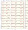 |
Fig. 11 Same as Fig. 10 for Fe iv– vi lines (from left to right panels, marked blue in the top panels) only. |
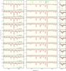 |
Fig. 12 Same as Fig. 10 for Ni iv– vi lines (from left to right panels, marked green in the top panels) only. |
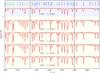 |
Fig. 23 Comparison of our model spectra (all calculated with log g = 7.60) with the STIS observation. Top: final homogeneous model (TMAP). The stratified NGRT models have Teff = 65 000 K, 60 000 K, 55 000 K, and 50 000 K (from top to bottom). The lines in the models are marked. |
Statistics of our model atoms.
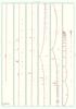 |
Fig. A.1 Comparison of the FUSE observation with our final model. Stellar and interstellar lines are identified. “is” denotes interstellar origin, “unid.” denotes unidentified lines. |
 |
Fig. A.2 Comparison of a section of the STIS observation with our final model. Stellar and interstellar lines are identified. “is” denotes interstellar origin, “unid.” denotes unidentified lines. |
Tübingen Model-Atmosphere WWW Interface, http://astro.uni-tuebingen.de/~TMAW
Acknowledgments
TR is supported by the German Aerospace Center (DLR, grant 05 OR 1301). The GAVO project at Tübingen has been supported by the Federal Ministry of Education and Research (BMBF, grants 05 AC 6 VTB, 05 AC 11 VTB). AstroGrid-D was funded by the BMBF (01 AK 804 [A-G]). The bwGRiD22 is funded within the framework of the D-Grid Project by the BMBF. This research has made use of the SIMBAD database, operated at the CDS, Strasbourg, France. This research has made use of NASA’s Astrophysics Data System. This work used the WRPLOT visualization software developed by Wolf-Rainer Hamann (Potsdam) and the WRPLOT team. Some of the data presented in this paper were obtained from the Mikulski Archive for Space Telescopes (MAST). STScI is operated by the Association of Universities for Research in Astronomy, Inc., under NASA contract NAS5-26555. Support for MAST for non-HST data is provided by the NASA Office of Space Science via grant NNX09AF08G and by other grants and contracts. The TEUV tool (http://astro-uni-tuebingen.de/~TEUV) used to apply interstellar corrections to theoretical spectra was constructed as part of the activities of the German Astrophysical Virtual Observatory. The TIRO service (http://astro-uni-tuebingen.de/~TIRO) used to calculate opacities for this paper was constructed as part of the activities of the German Astrophysical Virtual Observatory.
References
- Allen de Prieto, C., Hubeny, I., & Smith, J. A. 2009, MNRAS, 396, 759 [NASA ADS] [CrossRef] [Google Scholar]
- Anderson, E., & Francis, C. 2012, Astron. Lett., 38, 331 [NASA ADS] [CrossRef] [Google Scholar]
- Asplund, M., Grevesse, N., Sauval, A. J., & Scott, P. 2009, ARA&A, 47, 481 [NASA ADS] [CrossRef] [Google Scholar]
- Barstow, M. A., & Hubeny, I. 1998, MNRAS, 299, 379 [NASA ADS] [CrossRef] [Google Scholar]
- Barstow, M. A., Hubeny, I., & Holberg, J. B. 1998, MNRAS, 299, 520 [NASA ADS] [CrossRef] [Google Scholar]
- Barstow, M. A., Holberg, J. B., Hubeny, I., et al. 2001, MNRAS, 328, 211 [NASA ADS] [CrossRef] [Google Scholar]
- Barstow, M. A., Good, S. A., Holberg, J. B., et al. 2003, MNRAS, 341, 870 [NASA ADS] [CrossRef] [Google Scholar]
- Barstow, M. A., Cruddace, R. G., Kowalski, M. P., et al. 2005, MNRAS, 362, 1273 [NASA ADS] [CrossRef] [Google Scholar]
- Bauer, F., & Husfeld, D. 1995, A&A, 300, 481 [NASA ADS] [Google Scholar]
- Berengut, J. C., Flambaum, V. V., Ong, A., et al. 2013, Phys. Rev. Lett., 111, 010801 [NASA ADS] [CrossRef] [Google Scholar]
- Beuermann, K., Burwitz, V., & Rauch, T. 2006, A&A, 458, 541 [NASA ADS] [CrossRef] [EDP Sciences] [Google Scholar]
- Beuermann, K., Burwitz, V., & Rauch, T. 2008, A&A, 481, 769 [NASA ADS] [CrossRef] [EDP Sciences] [Google Scholar]
- Bohlin, R. C. 2007, in The Future of photometric, spectrophotometric and polarimetric standardization, ed. C. Sterken, ASP Conf. Ser., 364, 315 [Google Scholar]
- Bohlin, R. C., Dickinson, M. E., & Calzetti, D. 2001, AJ, 122, 2118 [NASA ADS] [CrossRef] [Google Scholar]
- Chayer, P., Fontaine, G., & Wesemael, F. 1995, ApJS, 99, 189 [NASA ADS] [CrossRef] [Google Scholar]
- Chayer, P., Vennes, S., Pradhan, A. K., et al. 1996, in Astrophysics in the extreme ultraviolet, eds. S. Bowyer, & R. F. Malina, IAU Colloq. 152, 211 [Google Scholar]
- Cruddace, R. G., Kowalski, M. P., Yentis, D., et al. 2002, ApJ, 565, 47 [NASA ADS] [CrossRef] [Google Scholar]
- Cutri, R. M., Skrutskie, M. F., van Dyk, S., et al. 2003, VizieR Online Data Catalog, II/246 [Google Scholar]
- Dickinson, N. J., Barstow, M. A., & Hubeny, I. 2012a, MNRAS, 421, 3222 [NASA ADS] [CrossRef] [Google Scholar]
- Dickinson, N. J., Barstow, M. A., Welsh, B. Y., et al. 2012b, MNRAS, 423, 1397 [NASA ADS] [CrossRef] [Google Scholar]
- Dreizler, S., & Wolff, B. 1999, A&A, 348, 189 [NASA ADS] [Google Scholar]
- Dupuis, J., Vennes, S., Bowyer, S., Pradhan, A. K., & Thejll, P. 1995, ApJ, 455, 574 [NASA ADS] [CrossRef] [Google Scholar]
- Finley, D. S., Basri, G., & Bowyer, S. 1990, ApJ, 359, 483 [NASA ADS] [CrossRef] [Google Scholar]
- Finley, D. S., Koester, D., & Basri, G. 1997, ApJ, 488, 375 [NASA ADS] [CrossRef] [Google Scholar]
- Fitzpatrick, E. L. 1999, PASP, 111, 63 [NASA ADS] [CrossRef] [Google Scholar]
- Giammichele, N., Bergeron, P., & Dufour, P. 2012, ApJS, 199, 29 [NASA ADS] [CrossRef] [Google Scholar]
- Gianninas, A., Bergeron, P., & Ruiz, M. T. 2011, ApJ, 743, 138 [NASA ADS] [CrossRef] [Google Scholar]
- Green, J., Jelinsky, P., & Bowyer, S. 1990, ApJ, 359, 499 [NASA ADS] [CrossRef] [Google Scholar]
- Groenewegen, M. A. T., & Lamers, H. J. G. L. M. 1989, A&AS, 79, 359 [NASA ADS] [Google Scholar]
- Gunderson, K., Wilkinson, E., Green, J. C., & Barstow, M. A. 2001, ApJ, 562, 992 [NASA ADS] [CrossRef] [Google Scholar]
- Guseinov, O. K., Novruzova, K. I., & Rustamov, I. S. 1983, Ap&SS, 96, 1 [NASA ADS] [CrossRef] [Google Scholar]
- Heber, U., Hamann, W.-R., Hunger, K., et al. 1984a, A&A, 136, 331 [NASA ADS] [Google Scholar]
- Heber, U., Hunger, K., Jonas, G., & Kudritzki, R. P. 1984b, A&A, 130, 119 [NASA ADS] [Google Scholar]
- Heber, U., Moehler, S., Napiwotzki, R., Thejll, P., & Green, E. M. 2002, A&A, 383, 938 [NASA ADS] [CrossRef] [EDP Sciences] [Google Scholar]
- Høg, E., Fabricius, C., Makarov, V. V., et al. 2000, A&A, 355, L27 [NASA ADS] [Google Scholar]
- Holberg, J. B., Wesemael, F., & Basile, J. 1986, ApJ, 306, 629 [NASA ADS] [CrossRef] [Google Scholar]
- Holberg, J. B., Kidder, K., Liebert, J., & Wesemael, F. 1989, in White dwarfs, Lect. Notes Phys. 328, ed. G. Wegner (Berlin: Springer Verlag), IAU Colloq., 114, 188 [Google Scholar]
- Holberg, J. B., Ali, B., Carone, T. E., & Polidan, R. S. 1991, ApJ, 375, 716 [NASA ADS] [CrossRef] [Google Scholar]
- Holberg, J. B., Hubeny, I., Barstow, M. A., et al. 1994, ApJ, 425, L105 [NASA ADS] [CrossRef] [Google Scholar]
- Holberg, J. B., Barstow, M. A., & Sion, E. M. 1998, ApJS, 119, 207 [NASA ADS] [CrossRef] [Google Scholar]
- Holberg, J. B., Barstow, M. A., Hubeny, I., et al. 2003, in Hubble’s science legacy: future optical/ultraviolet astronomy from space, eds. K. R. Sembach, J. C. Blades, G. D. Illingworth, & R. C. Kennicutt, Jr., ASP Conf. Ser., 291, 383 [Google Scholar]
- Holberg, J. B., Sion, E. M., Oswalt, T., et al. 2008, AJ, 135, 1225 [NASA ADS] [CrossRef] [Google Scholar]
- Hubeny, I., & Lanz, T. 1995, ApJ, 439, 875 [Google Scholar]
- Hubeny, I., Hummer, D. G., & Lanz, T. 1994, A&A, 282, 151 [NASA ADS] [Google Scholar]
- Hummer, D. G., & Mihalas, D. 1988, ApJ, 331, 794 [NASA ADS] [CrossRef] [Google Scholar]
- Kilkenny, D., Heber, U., & Drilling, J. S. 1988, South African Astronomical Observatory Circular, 12, 1 [Google Scholar]
- Kimble, R. A., Davidsen, A. F., Blair, W. P., et al. 1993, ApJ, 404, 663 [NASA ADS] [CrossRef] [Google Scholar]
- Koester, D. 1991, in Evolution of stars: the photospheric abundance connection, eds. G. Michaud, & A. V. Tutukov, IAU Symp., 145, 435 [Google Scholar]
- Koester, D., & Finley, D. 1992, in The Atmospheres of early-type stars, eds. U. Heber, & C. S. Jeffery (Berlin: Springer Verlag), Lect. Notes Phys., 401, 314 [Google Scholar]
- Koester, D., Schulz, H., & Weidemann, V. 1979, A&A, 76, 262 [NASA ADS] [Google Scholar]
- Kurucz, R. L. 1991, in NATO ASIC Proc. 341: Stellar atmospheres – beyond classical models, eds. L. Crivellari, I. Hubeny, & D. G. Hummer (Dordrecht: Reidel Publishing Co.), 441 [Google Scholar]
- Kurucz, R. L. 2009, in Am. Inst. Phys. Conf. Ser., eds. I. Hubeny, J. M. Stone, K. MacGregor, & K. Werner, 1171, 43 [Google Scholar]
- Kurucz, R. L. 2011, Can. J. Phys., 89, 417 [NASA ADS] [CrossRef] [Google Scholar]
- Kwok, S., Purton, C. R., & Fitzgerald, P. M. 1978, ApJ, 219, L125 [NASA ADS] [CrossRef] [Google Scholar]
- Lajoie, C.-P., & Bergeron, P. 2007, ApJ, 667, 1126 [NASA ADS] [CrossRef] [Google Scholar]
- Landolt, A. U., & Uomoto, A. K. 2007, AJ, 133, 768 [NASA ADS] [CrossRef] [Google Scholar]
- Lanz, T., Barstow, M. A., Hubeny, I., & Holberg, J. B. 1996, ApJ, 473, 1089 [NASA ADS] [CrossRef] [Google Scholar]
- Latour, M., Fontaine, G., Chayer, P., & Brassard, P. 2013, ApJ, 773, 84 [NASA ADS] [CrossRef] [Google Scholar]
- Lemoine, M., Vidal-Madjar, A., Hébrard, G., et al. 2002, ApJS, 140, 67 [NASA ADS] [CrossRef] [Google Scholar]
- Liebert, J., Bergeron, P., & Holberg, J. B. 2005, ApJS, 156, 47 [NASA ADS] [CrossRef] [Google Scholar]
- McCook, G. P., & Sion, E. M. 1999, ApJS, 121, 1 [NASA ADS] [CrossRef] [Google Scholar]
- Morton, D. C. 2000, ApJS, 130, 403 [NASA ADS] [CrossRef] [MathSciNet] [Google Scholar]
- Napiwotzki, R., & Rauch, T. 1994, A&A, 285, 603 [NASA ADS] [Google Scholar]
- Oegerle, W. R., Jenkins, E. B., Shelton, R. L., Bowen, D. V., & Chayer, P. 2005, ApJ, 622, 377 [NASA ADS] [CrossRef] [Google Scholar]
- Pancino, E., Altavilla, G., Marinoni, S., et al. 2012, MNRAS, 426, 1767 [NASA ADS] [CrossRef] [Google Scholar]
- Preval, S. P., Barstow, M. A., Holberg, J. B., & Dickinson, N. J. 2013, in ASP Conf. Ser. 469, eds. J. Krzesiński, G. Stachowski, P. Moskalik, & K. Bajan, 193 [Google Scholar]
- Rauch, T. 1997, A&A, 320, 237 [NASA ADS] [Google Scholar]
- Rauch, T. 2003, A&A, 403, 709 [NASA ADS] [CrossRef] [EDP Sciences] [Google Scholar]
- Rauch, T. 2008a, in Proc. Astronomical Spectroscopy and Virtual Observatory, eds. M. Guainazzi, & P. Osuna (European Space Agency), 183 [Google Scholar]
- Rauch, T. 2008b, A&A, 481, 807 [NASA ADS] [CrossRef] [EDP Sciences] [Google Scholar]
- Rauch, T. 2012 [arXiv:1210.7636] [Google Scholar]
- Rauch, T., & Deetjen, J. L. 2003, in Stellar atmosphere modeling, eds. I. Hubeny, D. Mihalas, & K. Werner, ASP Conf. Ser., 288, 103 [Google Scholar]
- Rauch, T., & Nickelt, I. 2009, in Multi-wavelength Astronomy and Virtual Observatory, eds. D. Baines, & P. Osuna, 49 [Google Scholar]
- Rauch, T., & Ringat, E. 2011, in Astronomical data analysis software and systems XX, eds. I. N. Evans, A. Accomazzi, D. J. Mink, & A. H. Rots, ASP Conf. Ser., 442, 563 [Google Scholar]
- Rauch, T., Ziegler, M., Werner, K., et al. 2007, A&A, 470, 317 [NASA ADS] [CrossRef] [EDP Sciences] [Google Scholar]
- Rauch, T., Nickelt, I., Stampa, U., Demleitner, M., & Koesterke, L. 2009, in Astronomical data analysis software and systems XVIII, eds. D. A. Bohlender, D. Durand, & P. Dowler, ASP Conf. Ser., 411, 388 [Google Scholar]
- Rauch, T., Ringat, E., & Werner, K. 2010 [arXiv:1011.3628] [Google Scholar]
- Rauch, T., Werner, K., Biémont, É., Quinet, P., & Kruk, J. W. 2012, A&A, 546, A55 [NASA ADS] [CrossRef] [EDP Sciences] [Google Scholar]
- Renedo, I., Althaus, L. G., Miller Bertolami, M. M., et al. 2010, ApJ, 717, 183 [NASA ADS] [CrossRef] [Google Scholar]
- Ringat, E., & Rauch, T. 2010, in Am. Inst. Phys. Conf. Ser., 1273, eds. K. Werner, & T. Rauch, 121 [Google Scholar]
- Ringat, E., Rauch, T., & Werner, K. 2012, Baltic Astron., 21, 341 [NASA ADS] [Google Scholar]
- Sahu, M. S., Landsman, W., Bruhweiler, F. C., et al. 1999, ApJ, 523, L159 [NASA ADS] [CrossRef] [Google Scholar]
- Savitzky, A., & Golay, M. J. E. 1964, Anal. Chem., 36, 1627 [NASA ADS] [CrossRef] [Google Scholar]
- Schuh, S. L., Dreizler, S., & Wolff, B. 2002, A&A, 382, 164 [NASA ADS] [CrossRef] [EDP Sciences] [Google Scholar]
- Seaton, M. J., Yan, Y., Mihalas, D., & Pradhan, A. K. 1994, MNRAS, 266, 805 [NASA ADS] [CrossRef] [Google Scholar]
- Shipman, H. L. 1979, ApJ, 228, 240 [NASA ADS] [CrossRef] [Google Scholar]
- Tremblay, P.-E., & Bergeron, P. 2009, ApJ, 696, 1755 [NASA ADS] [CrossRef] [Google Scholar]
- van Leeuwen, F. 2007, A&A, 474, 653 [NASA ADS] [CrossRef] [EDP Sciences] [Google Scholar]
- Vennes, S., & Lanz, T. 2001, ApJ, 553, 399 [NASA ADS] [CrossRef] [Google Scholar]
- Vennes, S., Thejll, P., & Shipman, H. L. 1991, in NATO ASIC Proc. 336, White dwarfs, eds. G. Vauclair, & E. Sion, 235 [Google Scholar]
- Vennes, S., Chayer, P., Hurwitz, M., & Bowyer, S. 1996, ApJ, 468, 898 [NASA ADS] [CrossRef] [Google Scholar]
- Vennes, S., Polomski, E. F., Lanz, T., et al. 2000, ApJ, 544, 423 [NASA ADS] [CrossRef] [Google Scholar]
- Vennes, S., Chayer, P., & Dupuis, J. 2005, ApJ, 622, L121 [NASA ADS] [CrossRef] [Google Scholar]
- Vernet, J., Kerber, F., D’Odorico, S., et al. 2008a, in 2007 ESO Instrument Calibration Workshop, eds. A. Kaufer, & F. Kerber (Heidelberg, Berlin: Spring Verlag), 153 [Google Scholar]
- Vernet, J., Kerber, F., Saitta, F., et al. 2008b, in Proc. SPIE, 7016 [Google Scholar]
- Vernet, J., Kerber, F., Mainieri, V., et al. 2010, Highlights of Astronomy, 15, 535 [NASA ADS] [Google Scholar]
- Vernet, J., Dekker, H., D’Odorico, S., et al. 2011, A&A, 536, A105 [NASA ADS] [CrossRef] [EDP Sciences] [Google Scholar]
- Vidal-Madjar, A., Allard, N. F., Koester, D., et al. 1994, A&A, 287, 175 [NASA ADS] [Google Scholar]
- Vidal-Madjar, A., Lemoine, M., Ferlet, R., et al. 1998, A&A, 338, 694 [NASA ADS] [Google Scholar]
- Wassermann, D., Werner, K., Rauch, T., & Kruk, J. W. 2010, A&A, 524, A9 [NASA ADS] [CrossRef] [EDP Sciences] [Google Scholar]
- Werner, K., & Dreizler, S. 1994, A&A, 286, L31 [NASA ADS] [Google Scholar]
- Werner, K., Deetjen, J. L., Dreizler, S., et al. 2003, in Stellar atmosphere modeling, eds. I. Hubeny, D. Mihalas, & K. Werner, ASP Conf. Ser., 288, 31 [Google Scholar]
- Werner, K., Rauch, T., Ringat, E., & Kruk, J. W. 2012, ApJ, 753, L7 [NASA ADS] [CrossRef] [Google Scholar]
- Wolff, B., Koester, D., Dreizler, S., & Haas, S. 1998, A&A, 329, 1045 [NASA ADS] [Google Scholar]
- Ziegler, M., Rauch, T., Werner, K., Köppen, J., & Kruk, J. W. 2012, A&A, 548, A109 [NASA ADS] [CrossRef] [EDP Sciences] [Google Scholar]
All Tables
Wavelengths (in Å) of unidentified strong (Wλ > 10 mÅ), likely photospheric lines in the FUSE and STIS observations.
Standard star SEDs (references for Teff and log g are given) presently available in TheoSSA.
All Figures
|
Fig. 2 Comparison of STIS and FUSE observations around H i L α–δ with our final model. Thick (red in the online version) photospheric + ISM line absorption model with NH i = 2.2 × 1018 cm-2; thin (blue) pure photospheric model; dashed (green, L α only) NH i = 1.2 × 1018 cm-2, 3.2 × 1018 cm-2. The locations of the D i blends are marked. L β–δ are shifted in flux (0.7, 1.6, 2.7 × 10⁻¹¹ erg cm-2 s-1 Å-1) for clarity. A reddening of EB − V = 0.0005 is applied following the law of Fitzpatrick (1999, with RV = 3.1. |
| In the text | |
|
Fig. 3 STIS spectrum around the interstellar absorption lines O iλ 1302.163 Å (top) and N iλλ 1199.550,1200.223,1200.710 Å (bottom) compared with the synthetic spectrum of our final model where the ISM lines are included. The labels give the radial velocities (in km s-1) that are applied. |
| In the text | |
|
Fig. 4 Comparison of FUSE and HST (STIS and NICMOS) observations with our final model. A reddening of EB − V = 0.0005 is applied. The low-resolution (LR) STIS+NICMOS observation vanishes behind the model SED due to the line width. Therefore, we plotted the observed spectrum twice, one shifted by Δlog fλ = −0.2 for clarity. U,R,I (Landolt & Uomoto 2007), B,V (Høg et al. 2000), J,H, and K (Cutri et al. 2003) fluxes (converted from brightnesses using values given by Heber et al. 2002) are shown for comparison. |
| In the text | |
|
Fig. 5 Occupation probabilities of the H i levels with principal quantum numbers n = 1 − 14 in our final model. |
| In the text | |
|
Fig. 7 Section of the FUSE observation compared with our model fluxes with different Teff and log g. In the top and middle panels, the synthetic fluxes are normalized to the observed flux at 1000 Å and in the bottom panel to the observed K magnitude (see Fig. 4). EB − V and NH i are applied using our results from Sect. 2.3. |
| In the text | |
|
Fig. 8 Synthetic H i Balmer-line profiles compared with the STIS LR observation. The observation is shifted by factors of 0.921, 0.323, 0.232, 0.202, 0.193, and 0.188 for Hα – Hζ, respectively, to fit into this plot. Red, full line: and log g = 7.60; blue, dashed: and log g = 7.55. |
| In the text | |
|
Fig. 9 STIS Hα and Hβ low-resolution (dashed, blue) and medium-resolution (gray lines) observations (labeled with medium-resolution grating/central wavelength in Å). Because of uncertainty in the flux calibration, the medium-resolution data are normalized to the low-resolution flux. The flux around Hβ in the top plot is multiplied by a factor of 0.35. The red lines in the upper two plots are the medium-resolution (R ≈ 6000) spectra degraded to the low resolution (R ≈ 500) and agree with the low resolution (blue dash) within the uncertainty of the R = 500 resolution. The lower two plots are shifted down by 0.035 and 0.07 × 10⁻¹³ flux units, respectively. In the lowest plot, the model is overplotted in red after smoothing to the medium resolution. While the model Hα absorption is somewhat too weak, the central emission agrees with the observation within the uncertainty of the resolution (insert). |
| In the text | |
|
Fig. 13 Synthetic spectrum around He iiλ 1640.42 Å compared with the STIS observation. He abundances are green, dashed: −10.0, red, thick: −4.7, blue, thin: −4.2, blue, dashed: −3.1. The insert shows the region Δλ = ± 0.4 Å around the He ii line. For comparison, the observation was smoothed with a low-pass filter (Savitzky & Golay 1964, n = 15, m = 4). |
| In the text | |
|
Fig. 14 Most prominent O iv, O v, and O vi lines in the STIS and FUSE observations compared with our theoretical line profiles calculated with three O abundances (O = −4.72, –5.12, –6.24, from top to bottom). |
| In the text | |
|
Fig. 15 Theoretical Al iii line profiles calculated from our final model compared with the STIS observation. |
| In the text | |
|
Fig. 16 Flux ratio of our final model and a model with ten times increased abundance of element X (Ca to Co, from top to bottom). The location of V ivλ1272.98 Å is marked. |
| In the text | |
|
Fig. 17 Theoretical line profiles of the strongest Zn iv lines in the STIS wavelength range compared with the observation. |
| In the text | |
|
Fig. 18 Top: photospheric abundances of G191−B2B (red stars) compared with solar values (Asplund et al. 2009). [X] denotes log (mass fraction/solar mass fraction) of element X. The dashed, green line shows the solar ratio. The arrows indicate upper limits. The cyan diamonds (Holberg et al. 2003), triangles (Vennes et al. 1996), and tridents (Vennes et al. 2005) are previously determined values. Bottom: comparison of our abundance number ratios (red stars) with predictions of diffusion calculations for DA-type (blue squares) WDs (Chayer et al. 1995) with and log g = 7.5. |
| In the text | |
|
Fig. 19 Same as Fig. 14. Top: dashed, green TMAP (=chemically homogeneous) model with O = −4.72; thin, blue TMAP model with abundance profiles from Dreizler & Wolff (1999), thick, red NGRT (=diffusion) model. Bottom: thick, red NGRT model with an artificially reduced O abundance in the outer atmosphere. Note that in the NGRT models, the line strengths of the generic iron-group element (see text) are overestimated. |
| In the text | |
|
Fig. 20 Abundance profiles in our diffusion model (, log g = 7.60). Short-dashed (blue) lines: unrealistically high abundance of the generic iron-group element (IG, see text), thick (red) lines: reduced IG abundance, horizontal long-dashed, thin (cyan) lines: the abundances in our final homogeneous model. In the O panel, the thick dashed (green) line shows our modified O-abundance profile (see text). |
| In the text | |
|
Fig. 21 Temperature structures (, log g = 7.60) of a pure H model (thin, black), our final homogeneous model (thick, red), and a diffusion model (dashed, blue). The formation depths of the line cores of the lowest members of the H i Lyman and Balmer series, the C iv, N v, O vi, Si iv, and S vi resonance doublets, and our strategic O ivλλ 1338.634,1343.022,1343.526 Å and O vλ 1371.296 Å lines are marked. |
| In the text | |
|
Fig. 22 Optical depth τ = 1 in our final homogeneous model. |
| In the text | |
|
Fig. 24 Top: comparison of three synthetic spectra (Teff = 55 000, 60 000, and 65 000 K) of chemically homogeneous models with the EUVE observation. The wavelengths of ground-state absorption thresholds of He ions are indicated. Bottom: comparison of a stratified model with the observation. |
| In the text | |
|
Fig. 25 Location of G191−B2B in the log Teff–log g plane (the ellipse indicates the errors of our analysis) compared with evolutionary tracks for hydrogen-rich white dwarfs (Renedo et al. 2010) labeled with the respective stellar masses (in M⊙). |
| In the text | |
|
Fig. 26 Comparison of our final TMAP model (blue, thick) with a TMAW model (red, thin). Top: astrophysical fluxes at the stellar surface, middle: ratio TMAP/TMAW flux, bottom: normalized fluxes. |
| In the text | |
|
Fig. 27 Flux ratio of two TMAP models at the edge of the Teff and log g error ranges and our final model. |
| In the text | |
|
Fig. 28 Determined Teff and log g values in the last 34 years. Blue triangles denote analyses with LTE models, red squares those with NLTE models (Table 2). The result of Koester et al. (1979, log g = 5.95 is outside the top and bottom panels. |
| In the text | |
|
Fig. 1 Flow diagram of TheoSSA. The VO user sends an SED request to the GAVO database by entering the photospheric parameters. If a suitable model is available within the desired tolerance limits, it is offered as a results table. In case that the parameters are not exactly matched, the VO user may decide to calculate a model with the exact parameters. TMAW will start a model-atmosphere calculation at our institute’s (IAAT) PC cluster then. Extended model grids make use of computer resources that are provided by AstroGrid-D. As soon as the model is converged, the VO user can retrieve the SED table from the GAVO database. |
| In the text | |
|
Fig. 6 Temperature and density structure and ionizations fractions of our model with and log g = 7.60. IG denotes a generic model atom consisting of Ca, Sc, Ti, V, Cr, Mn, and Co. |
| In the text | |
|
Fig. 10 Synthetic line profiles of C iii– iv, N iii– v, Si iii– iv, P iv– v, S iv– v, and Ge iv– v calculated from models with 57 000 K ≤ Teff ≤ 62 000 K and log g = 7.6 compared with FUSE and STIS observations. The small horizontal bars, labeled with the element’s name, indicate Teff where the ionization balance is best reproduced. The lines are identified at the top. “is” denotes interstellar origin. In the cases of C iv λλ 1548,1550 Å, C iv λλ 1548,1550 Å, and Si iii λλ 1206.500,1206.555 Å, the photospheric line profile is shown by a dashed, blue line (for the model at the top only). |
| In the text | |
|
Fig. 11 Same as Fig. 10 for Fe iv– vi lines (from left to right panels, marked blue in the top panels) only. |
| In the text | |
|
Fig. 12 Same as Fig. 10 for Ni iv– vi lines (from left to right panels, marked green in the top panels) only. |
| In the text | |
|
Fig. 23 Comparison of our model spectra (all calculated with log g = 7.60) with the STIS observation. Top: final homogeneous model (TMAP). The stratified NGRT models have Teff = 65 000 K, 60 000 K, 55 000 K, and 50 000 K (from top to bottom). The lines in the models are marked. |
| In the text | |
|
Fig. A.1 Comparison of the FUSE observation with our final model. Stellar and interstellar lines are identified. “is” denotes interstellar origin, “unid.” denotes unidentified lines. |
| In the text | |
|
Fig. A.2 Comparison of a section of the STIS observation with our final model. Stellar and interstellar lines are identified. “is” denotes interstellar origin, “unid.” denotes unidentified lines. |
| In the text | |
Current usage metrics show cumulative count of Article Views (full-text article views including HTML views, PDF and ePub downloads, according to the available data) and Abstracts Views on Vision4Press platform.
Data correspond to usage on the plateform after 2015. The current usage metrics is available 48-96 hours after online publication and is updated daily on week days.
Initial download of the metrics may take a while.