| Issue |
A&A
Volume 560, December 2013
|
|
|---|---|---|
| Article Number | A54 | |
| Number of page(s) | 12 | |
| Section | Planets and planetary systems | |
| DOI | https://doi.org/10.1051/0004-6361/201322234 | |
| Published online | 05 December 2013 | |
Magnesium in the atmosphere of the planet HD 209458 b: observations of the thermosphere-exosphere transition region
1 Institut d’Astrophysique de Paris, UMR7095 CNRS, Université Pierre & Marie Curie, 98bis boulevard Arago, 75014 Paris, France
e-mail: This email address is being protected from spambots. You need JavaScript enabled to view it.
2 School of Physics, University of Exeter, Exeter, EX4 4QL, UK
3 CASA, Department of Astrophysical and Planetary Sciences, University of Colorado, Boulder, CO 80309, USA
4 Division of Geological and Planetary Sciences, California Institute of Technology, MC 170-25 1200, E. California Blvd., Pasadena, CA 91125, USA
5 Lunar and Planetary Lab, University of Arizona, Tucson, AZ 85721, USA
6 Observatoire de Genève, Université de Genève, 51 Chemin des Maillettes, 1290 Sauverny, Switzerland
7 Observatoire de Haute-Provence, CNRS/OAMP, 04870 Saint-Michel l’ Observatoire, France
8 Department of Earth and Space Science and Engineering, York University 4700 Keele street, Toronto, ON M3J1P3, Canada
Received: 9 July 2013
Accepted: 25 September 2013
Abstract
The planet HD 209458 b is one of the most well studied hot-Jupiter exoplanets. The upper atmosphere of this planet has been observed through ultraviolet/optical transit observations with H i observation of the exosphere revealing atmospheric escape. At lower altitudes just below the thermosphere, detailed observations of the Na i absorption line has revealed an atmospheric thermal inversion. This thermal structure is rising toward high temperatures at high altitudes, as predicted by models of the thermosphere, and could reach ~ 10 000 K at the exobase level. Here, we report new near ultraviolet Hubble Space Telescope/Space Telescope Imaging Spectrograph (HST/STIS) observations of atmospheric absorptions during the planetary transit of HD 209458 b. We report absorption in atomic magnesium (Mg i), while no signal has been detected in the lines of singly ionized magnesium (Mg ii). We measure the Mg i atmospheric absorption to be 6.2 ± 2.9% in the velocity range from − 62 to − 19 km s-1. The detection of atomic magnesium in the planetary upper atmosphere at a distance of several planetary radii gives a first view into the transition region between the thermosphere and the exobase, where atmospheric escape takes place. We estimate the electronic densities needed to compensate for the photo-ionization by dielectronic recombination of Mg+ to be in the range of 108−109 cm-3. Our finding is in excellent agreement with model predictions at altitudes of several planetary radii. We observe Mg i atoms escaping the planet, with a maximum radial velocity (in the stellar rest frame) of −60 km s-1. Because magnesium is much heavier than hydrogen, the escape of this species confirms previous studies that the planet’s atmosphere is undergoing hydrodynamic escape. We compare our observations to a numerical model that takes the stellar radiation pressure on the Mg i atoms into account. We find that the Mg i atoms must be present at up to ~7.5 planetari radii altitude and estimate an Mg i escape rate of ~3 × 10⁷ g s-1. Compared to previous evaluations of the escape rate of H i atoms, this evaluation is compatible with a magnesium abundance roughly solar. A hint of absorption, detected at low level of significance, during the post-transit observations, could be interpreted as a Mg i cometary-like tail. If true, the estimate of the absorption by Mg i would be increased to a higher value of about 8.8 ± 2.1%.
Key words: planetary systems / planets and satellites: atmospheres / techniques: spectroscopic / methods: observational
© ESO, 2013
1. Introduction
The first detection of an exoplanet atmosphere was accomplished by detecting sodium in the transiting hot-Jupiter HD 209458 b (Charbonneau et al. 2002). A few other atomic species have been identified in the evaporating upper atmosphere of this planet as well, including hydrogen, oxygen and carbon (Vidal-Madjar et al. 2003, 2004). An extended hydrogen envelope of this planet was also suggested by Hubble Space Telescope/Advanced Camera for Surveys (HST/ACS) observations (Ehrenreich et al. 2008), although these data were not significantly conclusive. The atmospheric escape mechanism has been identified to be an hydrodynamic “blow-off” (Vidal-Madjar et al. 2004). While Ben Jaffel et al. (2007) confirmed the detection of an extended upper atmosphere, the author debated the escape mechanism (see also Vidal-Madjar et al. 2008 and Ben Jaffel 2008). However, more recent observations obtained with the Hubble Space Telescope/Cosmic Origins Spectrograph (HST/COS) have independently confirmed the nature of the hydrodynamic escape mechanism for this planet (Linsky et al. 2010).
Interestingly, complementary observations of the exoplanet’s atmosphere have been secured at different wavelengths, hence probing different altitudes. Ballester et al. (2007) reported detection of H i from recombination via the Balmer jump, while Rayleigh scattering by H2 molecules has also been shown to be a likely explanation for the observed increase of planetary radii toward near-ultraviolet (NUV) wavelengths (Sing et al. 2008a,b; Lecavelier des Etangs et al. 2008b).
Complementary observations have also probed deeper in the atmosphere of HD 209458 b with signatures of molecular species detected using transit spectrophotometry (Knutson et al. 2007; Sing et al. 2008a) or dayside spectrum (Swain et al. 2009). From this spectrum, broad band signatures were interpreted as due to the presence of water vapor (Barman 2007); upper-limits on TiO/VO abundances at high altitude were estimated (Désert et al. 2008), and the thermosphere has also been revealed through a detailed analysis of the Na i line profile (Vidal-Madjar et al. 2011a,b). Near-infrared observations revealed the presence of molecules deeper in this planet’s atmosphere with detections of CO (Snellen et al. 2010) and H2O (Deming et al. 2013). Hot-Jupiter orbit so close to their parents stars that they are exposed to intense extreme ultraviolet (EUV) irradiation and strong stellar winds, which can shape their atmospheres (Lecavelier des Etangs et al. 2004). The high temperatures cause the atmosphere to escape rapidly, implying that the upper thermosphere is cooled primarily by adiabatic expansion (Yelle et al. 2004). One of the hottest exoplanets known is the hot-Jupiter, WASP-12b (Hebb et al. 2009). Fossati et al. (2010) and Haswell et al. (2012) have detected the escaping upper atmosphere of this planet using HST/COS spectra obtained in the NUV. In particular, their observations focused on the extra absorption observed in the Mg ii resonance line cores. These authors interpreted their results in the framework of hydrodynamical escape, similarly to the case of HD 209458 b. In general, UV transit observations have the potential to reveal the mass-loss rates of an exoplanet atmosphere (e.g., Ehrenreich & Désert 2011; Bourrier & Lecavelier des Etangs 2013).
Here, we report new observations of HD 209458 b’s extrasolar atmosphere in the NUV. This spectral domain is particularly rich in terms of the detection possibilities of high altitudes species, which have strong absorption signatures at these wavelengths. These observations were completed under the HST program (ID#11576, PI J.-M. Désert) completed with the Space Telescope Imaging Spectrograph (STIS) instrument between July and December 2010. Observing in the UV offers a great advantage, because of the strong opacity of atoms and ions in that spectral range and the ease in identifying the species that causes the observed absorption, in sharp contrast with the interleaved molecular bands in the near-infrared. We first report the observations and provide details on the instrumental systematics that affect these observations in Sect. 2, while we present the data analysis in Sect. 3. We discuss our findings and draw conclusions from our observations in the two last sections of the paper.
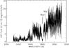 |
Fig. 1 Spectrum of HD 209458 over the whole observed spectral range. Many spectral signatures are seen in the stellar spectrum which includes the Mg ii doublet near 2800 Å, its core emissions due to the stellar chromosphere, and the strong Mg i line near 2850 Å. |
2. Observations and corrections
The observations were conducted using the Echelle E230M STIS grating, which provides a resolving power of λ/Δλ = 30 000. All observations were completed with the NUV-Multi-Anode Microchannel Array (NUV-MAMA) detector and a 0.2′′ × 0.2′′ entrance aperture, providing about 2 pixels per resolution element.
Three transits of HD 209458 b were observed; each used a succession of five consecutive HST orbits. Each HST orbit is built upon a similar observing sequence, producing ten successive exposures of 200 s each (except for the first orbits, which contain only nine exposures due to the time needed to the acquisition). Table 1 lists the observations log.
To compute the planetary orbital phase at the time of observation, we assumed a planet’s orbital period of 3.52474859 days and a central transit time of T0 = 53 344.768245 (MJD) (Knutson et al. 2007). The transits starts and ends at − 0.018 and + 0.018 planetary orbital phases, respectively. The mid-orbital phases shown in Table 1 give the positions of the five HST orbits during each transit: observations of orbits #1 and #2 are always before the transits, orbits #3 and #4 always during the transits, and orbit #5 always after the transits.
The spectra were extracted with the standard calstis pipeline (version 2.32), which includes localization of the orders, optimal order extraction, wavelength calibration, corrections of flat-field, etc. An example of this spectral extraction is shown in Fig. 1 with wavelengths between ~ 2300 Å and 3100 Å at the nominal spectral resolving power, which is at about 10 km s-1 resolution. These spectra contain large amounts of transitions, which gives a noisy appearance.
Log of the HST/STIS observations.
2.1. STIS echelle orders overlaps
Observations made with the E230M echelle spectrograph give access to several orders, covering the whole spectral domain but with some overlap at the extremity of these orders. In the overlapping spectral regions, we averaged the measurements obtained from the two different overlapping orders. At each orders edge, a few pixels (three consecutive ones, corresponding to about 15 km s-1 velocity domains or less than 0.15 Å wide) were found to be unreliable. For these pixels, we simply interpolated the spectrum measured at shorter and longer wavelengths, keeping track of these overlapping wavelengths. For instance, they are listed for transit #2 in Table 2. Because all three transits are not observed at the same epoch (i.e. at different heliocentric corrections, see Table 1), the three transits evaluated radial velocities in the heliocentric rest frame can present relative shifts up to the instrument spectral resolution of 10 km s-1.
E230M orders overlapping wavelengths for the transit #2 (in Å).
As a result, one should be careful to interpret any detected signature at the spectral orders edges, where an interpolation is done (covering ± 0.40 Å). When broad band spectral regions are considered (of about 200 Å), we find the potential perturbations are on the order of 0.1% of the studied signal and thus are considered negligible. In contrast, it is important to check that the positions of the order overlaps does not coincide with the studied domain for narrow spectral bands. In the present study, this is never the case.
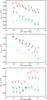 |
Fig. 2 Total HST flux of each sub-exposure measured over the 2900 − 3100 Å spectral domain as a function of the HST orbital phase (in erg cm-2 s-1). Upper plot: transit #1. During this transit, successive HST orbits are shown (orbit #2, black crosses, orbit #3, blue diamonds, orbit #4, green triangles and orbit #5, red squares). Middle plot: same as upper plot for transit #2. Lower plot: same as upper plot for transit #3. |
2.2. Orbital time series observations and correction of the STIS thermal “breathing” effect
For each transit observation, we discard data obtained during the first HST orbit, because systematic trends in the first orbit are found to be always significantly worse than in subsequent orbits; this is likely due to the fact that the HST must thermally relax into its new pointing position during this time. The procedure of discarding the first HST orbit of each transit is usually performed for HST observations of exoplanets’ transits (i.e., Sing et al. 2011; Huitson et al. 2012). For each HST orbit containing 10 sub-exposures, we also discard the first sub-exposures, which are always found to have an anomalous low flux.
The time series observations during each orbit are then extracted by adding the flux over a given spectral domain for each of the considered sub-exposures. As an example, this is shown in Fig. 2, where the total flux is summed over the 2900–3100 Å wavelength range for each sub-exposure of each orbit of each visit as a function of the HST orbital phase. Clear trends are seen that are repeated in all orbits. The correlation of the flux with the HST orbital phase is typical of the HST/STIS thermal “breathing” effect as the HST is heated and cooled during its orbit, causing focus variations.
The shape and amplitude of these systematic variations can change between visits of the same target, as has been found in the STIS optical transit observations of HD 209458 (Brown et al. 2001; Charbonneau et al. 2002; Sing et al. 2008a,b) and HD 189733 (Sing et al. 2011; Huitson et al. 2012). Extensive experience with the optical STIS data over the last decade further indicates that the orbit-to-orbit variations within a single visit are both stable and highly repeatable outside of the first orbit, which displays a different trend (see Brown et al. 2001 and Charbonneau et al. 2002). Because of its repeatability, this effect can be corrected.
It can be seen in Fig. 2 that all orbits in transits #1 and #2 show similar trends, although the observations obtained during the planet’s transit (the in-transit orbit: orbit #4) and during ingress (orbit #3) have lower baseline flux levels compared to the corresponding out-of-transit orbits; this is due to the planetary transit itself.
To correct for the systematic trends introduced by the HST “breathing” effect, the transit depths were fitted simultaneously with a 4th order polynomial function of HST orbital phase, which is referred to hereafter as the “breathing” correction. This correction has proved to be very successful for removing systematic trends in past observations using STIS (e.g., Sing et al. 2008a; Ehrenreich et al. 2012; Bourrier et al. 2013). We investigated whether higher order terms were justified by calculating the Bayesian information criterion (BIC), which is defined as χ2 + klnn for a normal distribution, where k is the number of free parameters and n is the number of data points. It was found that higher order terms that are greater than 4th order were not justified.
In the case of transit #3, the 4th order polynomial correction still leaves a ± 0.7% residual fluctuation (Fig. 3). When a better accuracy is required (i.e., for transit “absorption depths”, or ADs of the order of 1.5% or less), we ignore transit #3, which brings more noise than information. In contrast, for larger ADs, transit #3 is included in the analysis.
2.3. Baseline of the light curves and stellar activity
The variation in flux between orbits, as seen in transit #3, could be due to stellar variability. In the UV, where spectral lines can be very sensitive to the stellar activity, variations on the order of ± 1.5% in the UV are not unexpected. For example, some chromospheric lines can display variations of ~ 2 − 3% per hour as in the case of the Sun (see e.g. Vidal-Madjar 1975; Lemaire 1984).
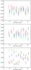 |
Fig. 3 Same as Fig. 2 for the fluxes of each sub-exposure normalized by the total flux that is measured during the transit and corrected for all trends as discussed (see text). Upper plot: transit #1. The overall fluctuation after correction is ± 0.2%. Middle plot: same as upper plot for transit #2. Overall fluctuation: ± 0.3%. Lower plot: same as upper plot for transit #3. Note here the different ordinate scale showing the relatively more perturbed transit #3. For that transit, the overall fluctuation is ± 0.7%. |
In the case of the Mg i and Mg ii spectral line studies presented here, it is known that the Mg ii line cores are formed from the higher parts of the photosphere to the upper part of the chromospheric plateau (Lemaire & Gouttebroze 1983), while the Mg i lines are formed in the upper part of the solar photosphere to the low chromosphere (Briand & Lemaire 1994). This means that the Mg ii line cores are more sensitive to stellar activity (in the case of a G2V star) than the Mg i line core. Because no significant variations are seen in the core of the Mg ii lines during transits (even during the third one, see Sect. 3.3) at a level of 2% at most, this means that we should expect even less perturbations due to stellar activity in the case of the Mg i line core study. Because the observed Mg i variations are above 6% (Sect. 3.2), we consider that variations due to stellar activity of the solar-like star HD 209458 are small enough to be properly corrected from now on, as was done with previous studies.
This comment also concerns the question of the stellar disk homogeneity. Such star-spot-like signatures, already seen in more active stars, could have some influence on the transit depth/shape and thus on the evaluations of the fitted parameters. The star HD 209458 which is of solar type and is quiet at the time of our observations since the Mg ii perturbation, is ~ 2%, any stellar disk inhomogeneity should affect less the Mg i (see spatial observations of the solar disk, e.g. Bonnet & Blamont 1968; Lemaire & Gouttebroze 1983). Again, Mg i show absorption signatures at the 6% level; these evaluations should not be affected significantly by possible stellar, spatial, or temporal activity.
In previous datasets (e.g., Sing et al. 2008a; Sing et al. 2011; Huitson et al. 2012), visit-long flux variations have been corrected by fitting a linear slope as a function of planetary phase for the baseline of the light curves during the entire visits. A simple linear slope over timescales of an HST-transit is found to be sufficient because stellar variability cycles have a typical duration of the order of several days. We also investigated the possibility of better fits to the data by light curves using higher degrees of the polynomial for the flux baseline. We found that the BIC does not improve significantly when using the 2nd degree polynomial for the baseline when binning the spectrum into 200 Å bins. For narrower spectral bands, the effect is even smaller. We therefore decided to use a linear function for the flux baseline in the fit to the light curves. This further shows that the stellar activity during our observations is low, as a perturbing stellar spot signature seen along the path of the planetary disk in front of the star would have led toward the selection of a higher degree polynomial.
2.4. Fit of the light curves and de-trending model
For all spectral bands used in the analysis presented in the following sections, we applied the breathing correction (a 4th order function of the HST phase) and a linear baseline for the out-of transit light curve to consider the visit-long stellar flux variations (linear function of the planetary phase). We used the model of Mandel & Agol (2000) to fit the transit light curve. The three transits were fitted simultaneously with the same functional form for the corrections but with separate correction parameters for each visit. One common value for the RP/R ⋆ parameter was used to fit all visits simultaneously. The orbital inclination of the system, central transit time, and a/R ⋆ are fixed to the values from Hayek et al. (2012).
The de-trending model used for each visit is described by  (1)where F0 is the baseline stellar flux level, a,b1,b2,b3, and b4 are constant fitted parameters, φ is planetary phase, and φHST is HST orbital phase (for the breathing correction). These parameters are found by a fit to the data; they are different for each of the three visits.
Finally, we use the Kurucz (1993) 1D ATLAS stellar atmospheric models1 and a 3-parameter limb darkening law to correct for the stellar limb darkening of the form: 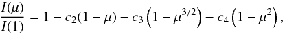 (2)where μ = cos (θ) and θ is the angle in radial direction from the disc center (see details in Sing 2010). The models were calculated at a very high resolution, R = 500 000, to ensure that the limb darkening could be well described for the numerous spectral lines in the data. We used T ∗ = 6000 K, log g = 4.5, and metallicity = 0.0 as the closest approximation to HD 209458. The limb-darkening coefficients are fixed when fitting the planet transit light curve.
2.5. Error estimation
To obtain an estimate of the absorption depth, (AD), that is translatable into a planetary radius, we have to use the complete de-trending model and include the limb-darkening correction to the fit of the data, as described in Sect. 2.4. However, the error bars produced by mpfit (Markwardt 2009), the code that we used to perform the simultaneous fit of the transit model and systematics correction, are an overestimate. Indeed, mpfit determines error bars using the full covariance matrix, which means that it considers the effect of each parameter on the other parameters. Such error estimates overestimate differential absorption depths if a large portion of the systematic trends are common mode. This is discussed in more details for a specific case (see below Sect. 3.2).
Therefore, we used the comparison between in-transit and out-transit spectra and calculated the corresponding absorption depth (ADIn/Out) to estimate the significance of a possible detected signal. By comparing the evaluated flux over any given bandpass, over which the stellar flux is averaged in a similar manner for orbits #2 and #5 (F2 + F5) on one hand and for orbits #3 and #4 (F3 + F4) on the other, we have access to the relative absorption depth (ADIn/Out):
 Using the errors provided by the STIS pipeline for each pixel of the corresponding observation, we can evaluate the error EIn/Out on the evaluated ADIn/Out:
 Because the orbits #4 are completed during the ingress of each of the three planetary transits, the ADIn/Out estimate is expected to be lower than the AD obtained through a full fit of the light curve (Sect. 2.4). Because the in/out ratio is free from uncertainties introduced by correlation in the parameters of the fit, it can be used to obtain estimates of error bars on differential absorption depths and detection significance levels.
3. Data analysis
3.1. Broadband transit absorption depths
We first looked for the transit signal over broad bands in the stellar continuum, which can be compared to the transit that is previously observed at longer wavelengths in the optical. At wavelengths of about 5000 Å, the depth of the transit light curve was measured to be AD ≈ (RP/R ∗ )2 = 1.444%, where RP and R ∗ are the planetary and stellar radii, respectively (Sing et al. 2008a, 2009). From the variation of AD between 4000 Å and 5000 Å and assuming that the absorption at these wavelengths is dominated by Rayleigh scattering in the planet atmosphere (see Lecavelier des Etangs et al. 2008a), the AD at 3000 Å is expected to be AD3000 ~ 1.484%. Using a fit to the data of transits #1 and #2 and the de-trending model as described in Sect. 2.4, we measured the planetary radii in 200 Å bins (Fig. 4). Here, we excluded the transit #3 data because it shows clear residual trends as a function of time (Sect. 2.2). Table 3 presents the coefficients as evaluated according to Eq. (1), and Table 4 shows the AD evaluated for the different spectral domains.
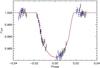 |
Fig. 4 Transit light curves over the broadband 2900–3100 Å that show the measurements obtained over each individual sub-exposure (black dots for transit #1, and blue dots for transit #2) as a function of the planet’s orbital phase. The first and last group of points, before and after the transit, around phase − 0.34 and +0.25 respectively, correspond to the Out of transit orbits #2 and #5, while the two other groups around phase − 0.15 and +0.05 correspond to the In transits observations that are completed respectively during orbit #3 (during ingress) and orbit #4 (deep within the transit). The solid red line shows the fitted profile, including limb-darkening and instrument breathing corrections. |
Broadband absorption depths (AD) measured over various spectral domains using the two first transit observations.
The AD measured here are consistent with the extrapolation, assuming Rayleigh scattering. However, our evaluations are not accurate enough to confirm that the variation of the AD as a function of wavelength follows the Rayleigh scattering law; a fortiori, this cannot be used to obtain an estimate of the atmospheric temperature. This limitation is mainly caused by the decrease in the stellar flux at short wavelengths, as can be seen in Table 4, where the errors clearly increase below 2700 Å.
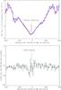 |
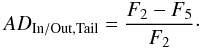
Fig. 5 Mg i line spectral region. Upper panel: the spectrum observed during the three transits. The average of orbits #2 and #5 (blue line) represent the Out of transit spectrum while the average of orbits #3 and #4 (red line) represent the In transit spectrum. Wavelengths are transformed into velocity shifts relative to the Mg i rest wavelength (individual pixels correspond to about 5 km s-1 bandwidth). Lower panel: the In/Out ratio of the two spectra (orbits #3 and #4 divided by orbits #2 and #5). The horizontal green line at the AD = 1.444% level corresponds to the Sing et al. (2008a) absorption depth evaluation at 5000 Å. The histogram shows the ratio rebinned over one resolution element which is over two instrument pixels (about 10 km s-1). The black dots give the ratios rebinned by 6 pixels with corresponding error bars, showing a single feature detected at more than 2-σ over a wide range of wavelengths. |
3.2. Mg i spectral absorption signature
Magnesium is an abundant species, and its neutral form presents a unique and strong spectral line, Mg i at 2852.9641 Å (Fig. 5). This deep line of about 500 km s-1 in width allows the measurement of the star radial velocity, which agrees with previous estimates (VStar = −14.7 km s-1; Kang et al. 2011).
In Fig. 5, the Out of the transit spectrum is the average of orbits #2 and #5, while the In transit one is the average of orbits #3 and #4. In both cases, these averages are completed over the three planet transit observations. The inclusion or exclusion of the third transit does not significantly alter the results. Around the Mg i line center, the In spectrum is seen to be lower than the Out spectrum (upper panel of Fig. 5). The In/Out ratio shows an excess absorption over several dozens of km s-1 in the blue side of the line (lower panel of Fig. 5). To evaluate precisely the absorption depth, we then use the fitting model described above.
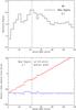 |
Fig. 6 Upper panel: maximum detection level of the absorption depth in the Mg i line as a function of the band width. The maximum detection level is reached at the σ-ratio of 2.1 for a band width of 43 km s-1 ± 3 km s-1 (AD = 6.2 ± 2.9%). Lower panel: velocity limits, Vmin (blue line) and Vmax (red line), of the band domains where the maximum of the significance level is reached as a function of the band width. Vmin is found to be roughly constant at about − 62 km s-1 (stellar reference frame). The position of the highest maximum signal-to-noise ratio at 43 km s-1 is shown by a vertical dashed line. |
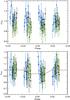 |
Fig. 7 Transit light curve measured in the − 62 to − 19 km s-1 spectral domain. The out-of-transit reference corresponds to the measurements in the orbits #2 (before transit) and #5 (after transit). Upper panel: raw observations. Lower panel: the limb-darkening and all trend correction that are included along with the final global fit (red solid line). All subexposures (black dots for transit #1, blue dots for transit #2 and green dots for transit #3) are shown. The evaluated AD that corresponds to the spectral domain is equal to 6.2 ± 2.9%. Note how flattened the limb-darkening looks: the reason being that the larger Mg i absorption gives a significantly larger planetary radius, which acts to smooth out the limb-darkening profile. |
3.2.1. De-trending model study
To determine the width and velocity of the Mg i absorption signature, as suspected from the ratio plot (lower panel of Fig. 5), we fitted the data using the de-trending model over the three transits and evaluated the AD for a variable spectral band width. We found the spectral position for which the ratio σ = AD/EAD is the largest, where EAD is the uncertainty on the measured absorption depth. As seen in Fig. 6, the strongest signature is found for a band width of 43 km s-1 extending from − 62 to − 19 km s-1. We note that the blue edge of the absorption domain is sharp, as shown by the constant value of the minimum velocity of the band that provides the largest σ-ratio for the absorption (Vmin around − 62 km s-1) and independent of the band width.
Since the evaluated absorption is over ~ 6% and much larger than the nearby continuum ADCont. levels (~1.5%), the transit #3 can be used in the estimates obtained above, because the data of this transit does not introduce more than ± 0.7% fluctuations.
The atmospheric Mg i transit signal over narrow bandpasses, which is in excess to the transit seen over large bandpasses and where Mg i does not absorb the stellar light, ADExcess, can be evaluated by comparing the total absorption depth (ADTotal) in the considered spectral region (i.e. near 2853 Å) to the absorption signature in the nearby continuum (ADCont.). The ADCont. is evaluated over two symmetric broad spectral domains (~2 Å wide) on both sides of the Mg i line (from − 2500 to − 500 km s-1 in the blue side of the line and from +500 to +2500 km s-1 in the red side). This leads to an average nearby stellar continuum absorption, ADCont. = 1.4 ± 0.1%.
To estimate the excess absorption in the spectral line due to the atmosphere only, this value must be subtracted to the total absorption measurement. From the estimated absorption depth ADTotal = 6.2 ± 2.9% and by using the relation, 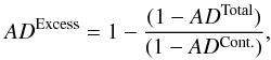 we evaluate an Mg i absorption excess of ADExcess = 4.9 ± 2.9%.
The whole de-trending model which includes the limb darkening correction, is adjusted over the observations for the spectral domain by providing the highest detection level for the absorption (from − 62 to − 19 km s-1; Fig. 7). We can however question the error bars estimates made via the fitting process because of the large number of parameters that are introduced and simultaneously fitted (breathing, light curve baseline, and the limb darkening corrections). To test these errors, we perturbed each parameter in the fit by ± 1σ and found that the ADExcess value changed by less than 0.1%, while the difference in ADTotal changed by 0.9% depending on the de-trending parameters used. We also found that a very similar spectrum as the one shown in Fig. 11 is produced by not fitting for trends at all. This seems to indicate that photon noise clearly dominates systematic noise in our small bins. Additionally, we found that the limb darkening correction made very little difference to the measured AD values; this is likely due to the large size of the planet’s effective radius and the flatness of limb darkening at this wavelength (and as seen by comparison of Figs. 4 and 7). The difference between the AD obtained with the limb darkening correction using the model coefficients and without the correction entirely changed the ADExcess value by only 0.5%.
3.2.2. ADIn/Out study
To further investigate the systematic effects, we evaluated the same absorption signatures by conducting a similar study at this wavelength range and using the ADIn/Out evaluations (Sect. 2.5). For the same spectral domain as above (from −62 to −19 km s-1), the In/Out estimates lead to a total absorption depth of  . The average stellar continuum absorption is
  . Thus, the Mg i absorption excess is
  . This corresponds to a detection level of the atmospheric Mg i of σIn/Out = 4.0.
Here, the detection level of the absorption signature of atmospheric Mg i is higher. This is not because the absorption depth value has changed (from 6.2 to 7.5%), but occurs when the error evaluation is significantly lower (from 2.9 to 1.6%). We can explain this result by the fact that the systematics are strongly tight together between the different orbits datasets and that their effect is almost washed out when comparisons are made between different orbits. They are even more washed out when relative ADExcess evaluations are made using the procedure of comparison between in-transit and out-transit data.
Using a planetary radius given by (RP/R∗)2 = 1.444%, an absorption of 7.5% corresponds to an opaque magnesium atmosphere that extends up to about 2.3 RP, an altitude level in the thermosphere/exosphere region where the blow off process starts to be effective (see e.g., Koskinen 2013a,b).
3.2.3. Significance and summary of the Mg i spectral absorption signature
We calculated the false-positive probability (FPP) to find a Mg i absorption excess that was at least as significant as the one detected in the data but caused by noise only. This requires defining a priori the kind of signatures that would be considered a posteriori as an atmospheric absorption feature. In particular, we need to define the wavelength range (and the corresponding velocity range) around the Mg i line center, where any absorption could be considered as a plausible absorption due to magnesium in the planet environment. Observationally, the highest velocity ever detected in an exoplanet atmosphere is − 230 km s-1 in the case of H i in the blue wing of the Lyman-alpha line (Lecavelier des Etangs et al. 2012). No absorption signature was also ever detected at more than +110 km s-1 in the red wing of a stellar line during transit observations (Bourrier et al. 2013). On the theoretical side, numerical simulations show that the radial velocity of a magnesium atom pushed by radiation pressure cannot exceed − 230 km s-1 when it transits in front of the stellar disk of HD 209458. We thus considered a conservative velocity range of [− 300; 150] km s-1, for which any absorption may have been interpreted as possibly caused by atmospheric magnesium. This conservative velocity range yields a FPP of 13%. Nonetheless, all the observed properties of the signature are well explained by our simple dynamical model (Sect. 4.3), which can explain absorption only within the velocity range [− 230; 0] km s-1. This velocity range yields a corresponding FPP of 6%. If we consider only the features with properties (velocity, strength, absorption profile) which can be reproduced by this model with plausible physical quantities (for ionization, escape rate, etc.) as a positive detection, the corresponding FPP would be even lower than 6% but this is difficult to quantify.
There is also an apparent absorption feature around 0 km s-1 in Fig. 5. This feature is spread over at most 4 pixels (two resolution elements). We also calculated its FPP and found that this feature has about 75% chance to be spurious and only due to statistical noise in the data.
3.3. Mg ii spectral absorption signature
With the detection of the Mg i signature (Sect. 3.2), the acknowledgement that ionized species have already been detected in the HD 209458 b planetary atmosphere (Vidal-Madjar et al. 2004; Linsky et al. 2010), and the acknowledgement that Mg ii was possibly detected in another extrasolar planet atmosphere (Fossati et al. 2010; Haswell et al. 2012), we thought there was a good prospect for the detection of ionized magnesium through the strong doublet at 2803.5305 Å (Mg ii-h) and 2796.3518 Å (Mg ii-k). The presence of a doublet is a clear advantage, because this allows us to check both lines for absorption signatures. With the doublet lines spectral separation translated into radial velocities on the order of 770 km s-1, any signal due to ionized magnesium with no more than a ± 400 km s-1 radial velocity separation benefits from two independent simultaneous observations.
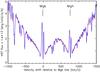 |
Fig. 8 Mg ii lines spectral region (Mg ii-k line at 2796.35 Å and Mg ii-h line at 2803.53 Å). The spectrum is observed during the two first transits. The average of orbits #2 and #5 (blue line) represents the Out of transit spectrum, while the average of orbits #3 and #4 (red line) represents the In transit spectrum. Wavelengths are transformed into velocity shifts relative to the Mg ii-k line (individual pixels correspond to about 5 km s-1 bandwidth). |
Figure 8 shows the spectral region of the Mg ii doublet. A self-reversed emission can be seen in the core of each line, which is due to the stellar chromosphere. Additional absorption at the center of that chromospheric emission is mainly due to the interstellar absorption, which is slightly redshifted relative to the star reference frame.
We searched for Mg ii absorptions using 43 km s-1 wide spectral domains (Fig. 9). We did not detect any Mg ii absorption down to 1% AD level. We found that the average absorption depth in all of the 43 km s-1 bins corresponds exactly to the absorption depth measured in the nearby stellar continuum. We also searched over broader and narrower domains and found no significant absorption signature. Finally, we also searched for Mg ii signatures independently within each of the three transits observations without any positive result.
The non-detection of excess absorption in the Mg ii lines (with upper limit of about 1% in AD) is in strong constrast with the Mg i detection with AD ~ 6.2–7.5% (Sect. 3.2). This shows that most of the magnesium must be neutral up to at least 2 RP distance from the planet center.
 |
Fig. 9 Absorption depth in 43 km s-1 band widths (histogram), as measured around the Mg ii doublet at ~ 2800 Å by using orbit #2 and #5 as the out-of-transit reference. The absorption depth is averaged over the two Mg ii lines. The absorption depth in the stellar continuum (dashed horizontal line) is measured using the two sides of the Mg ii doublet (from − 3000 to − 1000 km s-1 and from +1000 to +3000 km s-1). |
4. Discussion
4.1. Mg ii non-detection
The non-detection of Mg ii absorption from the planetary atmosphere cannot be interpreted by strong interstellar extinction as in the case of the WASP-12 system (Fossati et al. 2010; Haswell et al. 2012). Indeed, stellar Mg ii chromospheric emissions in the core of the two lines are clearly seen in the case of HD 209458, showing a low interstellar absorption. In light of the Fossati et al. (2010) early ingress detection of the planetary transits in the Mg ii lines, we searched for pre- or post-transit absorption signatures in the Mg ii light curve. We did not find any significant signal before or after the transit in neither the data of the orbits #2 nor of the orbits #5. As a result, we conclude that no Mg ii absorption is detected with an upper limit of 1% on the absorption depth.
4.2. Search for a cometary-like tail signature
Because a transit of a cometary-like tail can be observed after the planetary transit, which is possibly during orbit #5, we have compared orbit #2 (pre-transit) and orbit #5 (post-transit). For this we have evaluated the absorption depth due to the putative gaseous tail (ADIn/Out,Tail) by measuring the difference between the flux as measured before and after the transit:
 As expected, the evaluated differences are close to zero (Fig. 10). The average of the evaluations made over two symmetric broad spectral domains on both sides of the Mg i line (over the −2500 to −500 km s-1 blue domain and the +500 to +2500 km s-1 red domain) is also nearly equal to zero. However an outliers measurement near the Mg i line core is obtained at a maximum differential ADIn/Out,Tail of about 4.0 ± 2.2% over a blue-shifted, 81 km s-1 wide domain from − 67 to + 14 km s-1 in the stellar reference frame. This absorption signature, as detected in data collected after the planetary transit, suggests the presence of a tail of magnesium transiting after the planet.
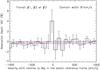 |
Fig. 10 Mg i ADIn/Out,Tail differences between the orbit #5 (before planetary transit) and the orbit #2 (after transit) using a 81 km s-1 band width (histogram). For comparison, the same differences have been measured in the stellar continuum blue-ward and red-ward of the Mg i line (blue and red lines, respectively). No differential absorption is detected, except in a single pixel that corresponds to a blue-shifted velocity domain from − 67 to + 14 km s-1 (see text). |
We also find that the average of the ADIn/Out,Tail differences estimated in the entire − 2500 to +2500 km s-1 spectral range (ignoring the 4% outlier) is equal to − 0.4 ± 0.4%. This shows that the stellar flux variations on the average over the three transits are negligible and that stellar activity and star spots are not a concern in our study, as previously discussed in Sect. 2.3.
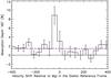 |
Fig. 11 Absorption depth in 43 km s-1 band widths (histogram), as measured around the Mg i line by using only the orbit #2 as the out-of-transit reference. The absorption depths measured in the stellar continuum in the +500 to +2500 km s-1 range (red side continuum, red dot-dashed line) and in the − 2500 to − 500 km s-1 range (blue side continuum, blue dashed line) are also shown. The AD′Total absorption depth is measured to be 8.8 ± 2.1% in the velocity domain from − 67 to − 19 km s-1. |
Because of this possible Mg i absorption in orbit #5, the estimates of the transit absorption that are obtained using a fit with a model of an opaque spherical body could be biased. We thus repeated the fitting process with a modified de-trending model, in which only orbit #2 is used as the out-of-transit reference. We note the corresponding absorption depths AD′ (Fig. 11). We obtain the following results: AD′Cont. = 1.3 ± 0.1%, AD′Total = 8.8 ± 2.1% (4.2σ), and AD′Excess = 7.5 ± 2.1%.
Using a planetary radius given by (RP/R ∗ )2 = 1.444%, an absorption of 8.8% corresponds to about 2.5 RP. However, the Mg i absorbing cloud of gas is likely asymmetric because the Mg i absorption is detected only in the blue wing of the line (between − 62 and − 19 km s-1); this possibility is strengthened by the detection of a tail transiting after the planetary body. Therefore, these values of Mg i altitude represent a lower limit and the detected Mg i atoms can be much higher in the planetary atmosphere.
4.3. Dynamics of escaping magnesium atoms
All theoretical models with hydrodynamical escape (e.g. Koskinen et al. 2013b and references there in) predict the blow-off escape velocity to be in the 1 to 10 km s-1 range (at ~ 2RP). Here, atomic magnesium is observed to be accelerated after release, reaching velocities in the range of − 62 to − 19 km s-1. In the exosphere, Mg i atoms are in a collisionless region and naturally accelerate away from the star by radiation pressure. As a result, magnesium atoms in the exosphere are expected to be at blue shifted velocities, as observed.
We have developed a numerical simulation, following those done for H i atoms (see Lecavelier des Etangs et al. 2012 for HD 189733 b; Bourrier & Lecavelier des Etangs 2013 for HD 189733 b and HD 209458 b) to calculate the dynamics of magnesium atoms. In the simulation, the Mg i particles are released from a level R0 within the atmosphere at the blow-off flow velocity, which is assumed to be 10 km s-1. The atoms’ dynamics are calculated by considering the gravity of the planet and the star, as well as the stellar radiation pressure. This last force acts in the opposite direction of the stellar gravity and progressively accelerates the particles away from the star up to velocities similar to the observed blue shifted atmospheric absorption. We also consider that radiation pressure is directly proportional to the velocity-dependent stellar flux, as seen by the moving particles. Because of the profile of the stellar line near the Mg i resonance line (Fig. 5) with a stronger flux away from the line center, the particle acceleration increases with their velocity blueward of the line. The Mg i atoms are ionized by the stellar flux but also recombined if the ambient electron volume density is high enough (see below). We represented the balance of these two effects by setting an ionization radius, Rion, above which magnesium atoms are all ionized. Above this cut-off radius, the electron volume density is too low to allow efficient recombination of Mg ii into Mg i. The third parameter of the simulation is the Mg i escape rate, Ṁ[Mg].
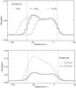 |
Fig. 12 Theoretical absorption depth of Mg i, as calculated using numerical simulations of the escape of magnesium atoms accelerated by stellar radiation pressure. Upper panel: AD as a function of the radial velocity for various ionization cut-off radii (in RP units). We find that a cut-off of 7.5 RP provides an AD profile that matches the velocity range of the observed absorption on the blue edge (indicated by the leftward vertical line); the other velocity limit shown is around 10 km s-1 (the other vertical line), which is independent of the radiation pressure model calculation, since it is related to the assumed blow-off velocity; this profile is obtained for a magnesium mass loss rate of 3 × 10⁷ g s-1. Lower panel: same as above for an ionization cut-off radius of 7.5 RP and two different Mg i escape rates. This shows that the two main parameters of the model (escape rate and cut-off radius) can be constrained independently through the measurement of the absorption depth and the velocity range of the gas. |
The results of the numerical simulation are shown in Fig. 12 with two varying parameters: Rion and dM/dt[Mg]. The parameter R0 was fixed at 2 RP at about the exobase level, where collisions become negligible (note that the value of R0 is found to have no significant impact on the results). Our first aim was to reproduce the sharp velocity limit of the detected absorption signature around − 60 km s-1 in the stellar reference frame. Our second goal was to reproduce the absorption depth measured in the Mg i line as a function of the radial velocity, especialy with the absorption of the velocity range [− 62; − 19 km s-1], which is measured to be about 6%. We found that the blueward velocity limit and the absorption depth can be fitted in a straightforward manner, because they are constrained independently by the cut-off radius and the escape rate, respectively (see Fig. 12). We found that our observations are well reproduced for Rion ~ 7.5 RP and dM/dt[Mg] ~ 3 × 10⁷ g s-1. Assuming a solar abundance of magnesium (~4 × 10⁻⁵ with respect to hydrogen, see Asplund et al. 2009), this last result corresponds to an H i escape rate from HD 209458 b of ~3 × 10¹⁰ g s-1. This is consistent with the escape rate of neutral hydrogen as derived from Lyman-α observations (see e.g., Lecavelier des Etangs et al. 2004; Ehrenreich et al. 2008; Bourrier & Lecavelier des Etangs 2013).
The planetary radius that corresponds to the AD of 6–8% (~2.5 RP) is different from the estimated cut-off radius Rion of Mg i at about 7.5 RP. This is explained because the 2.5 RP estimation assumes a cloud with a spherical symmetry, while the geometry of the occulting gas is not spherically symmetric but pushed by radiation pressure in a comet-like tail that trails behind the planet. Of course, this requires a cloud that is more extended on only one side to produce a similar absorption depth.
4.4. Magnesium ionization and recombination
The mere presence of atomic magnesium may appear surprising in the exosphere of HD 209458 b, because this neutral species has a low ionization potential of 7.65 eV. As a comparison to the HD 209458 b environment, carbon is found in its ionized form (Vidal-Madjar et al. 2004; Linsky et al. 2010), while the carbon ionization potential (11.26 eV) is larger than that for magnesium (7.65 eV).
However, there is a similar situation in the local interstellar medium, where neutral atomic magnesium is observed. To explain such a paradoxical situation, it was shown that the Mg ii recombination is extremely sensitive to the medium temperature (see Fig. 8 of Lallement et al. 1994). Indeed the dielectronic recombination rates of Mg ii steeply rises at temperatures above 6000 K (Jacobs et al. 1979). With this mechanism being the most effective to recombine Mg ii at temperature above ~ 3000 K, the balance between that recombination mechanism and all ionization mechanisms is such that Mg i can survive in this astrophysical environment.
In the planetary atmosphere, the detection of atomic magnesium through the Mg i line shows that the electronic volume density must be large enough to allow the Mg ii recombination to overcome all the possible ionization mechanisms. These ionization mechanisms are: i) the UV photo-ionization from the nearby star; ii) the electron-impact ionization (see e.g. Voronov 1997); iii) the charge-exchange of Mg i with protons (see e.g. Kingdon & Ferland 1996) and iv) the charge-exchange of Mg i with He ii.
Because the situation is certainly far from equilibrium in these upper parts of the atmosphere, the electron and proton volume densities are likely different. He ii may also play a non-negligible role. It is thus very difficult to evaluate the charge-exchange ionization rates. The electron-impact ionization may also be significant at very high temperatures. For instance, the ionization overcomes the dielectronic recombination at temperature above ~ 9000 K by using extrapolation of electron-impact ionization rates given by Voronov (1997). However, the rates given by Voronov (1997) are given for temperatures above ~ 11 000 K and may not apply at lower temperature regimes. Because of the large uncertainties on the effective rate of electronic ionization at temperatures below 11 000 K, we decided to consider both situations with and without this ionization mechanism (Fig. 13).
Among the ionization mechanisms, the photoionization can be easily calculated. To estimate ionizing UV flux at 0.047 AU from HD 209458, we used FHD 209458 b(λ), the stellar UV flux at wavelengths below the ionization threshold of 1621 Å as measured by Vidal-Madjar et al. (2004). The photoionization cross-section as a function of wavelength σion(λ) for the 3s2 [entity ! #x20 ! ] 1S ground state of Mg i is taken from Merle et al. (2011). We thus found the magnesium ionization rate to be
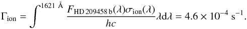 At the short orbital distance from the star, the magnesium is therefore quickly photoionized with a short timescale of about 0.6 h. The presence of atomic magnesium at altitudes up to several planetary radii from the planet can hence be explained only if the recombination is efficient enough to compensate for the ionization.
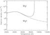 |
Fig. 13 Electron volume density needed to obtain the magnesium ionization equilibrium as a function of the temperature. At a lower density, the magnesium is mostly ionized, while the magnesium is mostly in its atomic form at higher density. The ionization rate is calculated using the electron-impact ionization rate extrapolated from the rate of Voronov (1997) that is combined with the photo-ionization rate (solid line) or the photo-ionization rate only (dashed line). |
The radiative and dielectronic recombination rates can be found in the literature. These recombination rates depend upon two atmospheric parameters: the electron temperature and the electron volume density (e.g., Frisch et al. 1990). The dielectronic recombination rate, αrec di, is highly temperature-dependent and quickly rises at temperatures above 6000 K. We used the dielectronic rate given by αrec di = 1.7 × 10⁻³T-1.5exp( − T0/T) cm3 s-1 with T0 = 5.1 × 10⁴ K and the radiative rate given by αrec rad = 1.4 × 10⁻¹³(T/104)-0.855 cm3 s-1 (Aldrovandi & Pequignot 1973). The total recombination rate is given by αrec = αrec di + αrec rad.
To estimate the electronic temperature and volume density needed to explain the detection of atomic magnesium, we calculated the ionization-recombination balance of magnesium exposed to the ionizing UV flux at 0.047 AU from HD 209458. Because of the unknown efficiency of ionization mechanisms other than photoionization, we decided to consider only photoionization and possibly the electron-impact ionization rate extrapolated from Voronov (1997). With this limitation, the calculated ionization rate is a lower limit, and the corresponding electron density is also a lower limit. This lower limit on the electronic density that is needed to obtain the magnesium ionization equilibrium is calculated as a function of the temperature (Fig. 13). It is noteworthy that the required electronic density must be above 108–109 cm-3. Considering the uncertainties in the modeling of the upper atmosphere and in the ionization/recombination rates, the possible effect of the unknown magnetic field, and the error bars on the Mg I detection, the electron density required is in reasonable agreement with the value estimated by Koskinen et al. (2013a; see their Fig. 9). This value is simply deduced from the Koskinen et al. (2013a) model proton density by assuming that the medium is neutral, which should be true somewhere below the altitudes considered here.
If the rise in electron-impact ionization efficiency, as given by Voronov (1997) applies to this temperature regime, we conclude that the temperature must be below ~9000 K (Fig. 13). The larger efficiency of the dielectroniic recombination also favors temperature above ~6000 K. Thus, the present detection of magnesium provides new constraints on the density and temperature, high in the exosphere of HD 209458 b, up to ~7.5 RP. Previously, the measurement of the temperature at the highest altitude in the thermosphere was obtained through analysis of the absorption in the core of the NaI line (Vidal-Madjar et al. 2011a,b); this constrained a temperature of ~3600 K at 10-7 bar, which corresponded to a density of ~2 × 1011 cm-3. Here, the detection of atomic magnesium, which requires high temperature and electron density at high altitudes in the atmosphere, extends the temperature-altitude profile in the thermosphere, which is already probed deeper through the sodium line profile. With a lower limit for the electron density of 108–109 cm-3 typical of the base of the exosphere and velocity characteristics of acceleration by radiation pressure, the detected magnesium atoms provide a new insight into the transition region between the upper part of the thermosphere and the bottom of the exosphere, where the atmospheric escape is taking place.
5. Conclusion
Here, we presented the detection of absorption in the Mg i line during the planetary transit, which is due to magnesium atoms at high altitude in the atmosphere of HD 209458 b. We measured an atmospheric absorption of 6.2 ± 2.9% in the velocity range from − 62 to − 19 km s-1, which presents a FPP of being due to noise of about 6%. In addition, no extra absorptions in the Mg ii lines were found with an upper limit of about one percent.
From this Mg i detection, we derived the following consequences:
-
The high ionization rate of magnesium by the stellar UV photons implies that dielectronic recombination of Mg ii must be efficient, which requires a high electronic density above 108–109 cm-3.
-
Because thermal escape of heavy species like magnesium is inefficient (even at 10 000 K), the detection of escaping magnesium confirms the scenario of an hydrodynamical escape (blow-off scenario).
-
A numerical simulation shows that the velocity range of observed magnesium is easily explained through acceleration by radiation pressure. Pushed away by radiation pressure, the magnesium must be in atomic form for distances up to about 7.5 planetary radii for the planet center.
-
This numerical simulation also allows an estimate of the magnesium escape rate of ~3 × 10⁷ g/s, which is consistent with the measured H i escape rate, if we assume a solar abundance.
-
Finally, a cometary tail geometry of the magnesium, as predicted by the numerical simulation, is possibly detected through residual absorption in the post-transit data. If true, the estimate of the absorption depth of Mg i must be revised to a higher value of about 8.8 ± 2.1%.
Acknowledgments
Based on observations made with the NASA/ESA Hubble Space Telescope, obtained at the Space Telescope Science Institute, which is operated by the Association of Universities for Research in Astronomy, Inc., under NASA contract NAS 5-26555. These observations are associated with program #11576. The authors acknowledge financial support from the Centre National d’Études Spatiales (CNES). The authors also acknowledge the support of the French Agence Nationale de la Recherche (ANR), under program ANR-12-BS05-0012 Exo-Atmos. J.-M.D. acknowledges funding from NASA through the Sagan Exoplanet Fellowship program administered by the NASA Exoplanet Science Institute (NExScI). D.K.S. and C.M.H. acknowledges support from STFC consolidated grant ST/J0016/1. D.E. acknowledges the funding from the European Commissions Seventh Framework Programme as a Marie Curie Intra-European Fellow (PIEF-GA-2011-298916). J. C. McConnell passed away on July 29, 2013. He was a highly respected scientist. We all would like to dedicate the present study to him. John “Jack” was more than a colleague, a friend; we deeply miss him. Jack was the first who understood that the atmospheric blow-off mechanism, which had never been directly observed before, as the phenomenon, takes place in the HD 209458 b atmosphere.
References
- Aldrovandi, S. M. V., & Pequignot, D. 1973, A&A, 25, 137 [NASA ADS] [Google Scholar]
- Asplund, M., Grevesse, N., Sauval, A. J., & Scott, P. 2009, ARA&A, 47, 481 [NASA ADS] [CrossRef] [Google Scholar]
- Ballester, G. E., Sing, D. K., & Herbert, F. 2007, Nature, 445, 511 [NASA ADS] [CrossRef] [Google Scholar]
- Barman, T. 2007, ApJ, 661, L191 [NASA ADS] [CrossRef] [Google Scholar]
- Ben-Jaffel, L. 2007, ApJ, 671, L61 [NASA ADS] [CrossRef] [Google Scholar]
- Ben-Jaffel, L. 2008, ApJ, 688, 1352 [NASA ADS] [CrossRef] [Google Scholar]
- Bonnet, R. M., & Blamont, J. E. 1968, Sol. Phys., 3, 64 [NASA ADS] [CrossRef] [Google Scholar]
- Bourrier, V., & Lecavelier des Etangs, A. 2013, A&A, 557, A124 [NASA ADS] [CrossRef] [EDP Sciences] [Google Scholar]
- Bourrier, V., Lecavelier des Etangs, A., Dupuy, H., et al. 2013, A&A, 551, A63 [NASA ADS] [CrossRef] [EDP Sciences] [Google Scholar]
- Briand, C., & Lemaire, P. 1994, A&A, 282, 621 [NASA ADS] [Google Scholar]
- Brown, T. M., Charbonneau, D., Gilliland, R. L., Noyes, R. W., & Burrows, A. 2001, ApJ, 552, 699 [NASA ADS] [CrossRef] [Google Scholar]
- Charbonneau, D., Brown, T. M., Noyes, R. W., & Gilliland, R. L. 2002, ApJ, 568, 377 [NASA ADS] [CrossRef] [Google Scholar]
- Deming, D., Wilkins, A., McCullough, P., et al. 2013, ApJ, 774, 95 [NASA ADS] [CrossRef] [Google Scholar]
- Désert, J.-M., Vidal-Madjar, A., Lecavelier des Etangs, A., et al. 2008, A&A, 492, 585 [NASA ADS] [CrossRef] [EDP Sciences] [Google Scholar]
- Ehrenreich, D., & Désert, J.-M. 2011, A&A, 529, A136 [NASA ADS] [CrossRef] [EDP Sciences] [Google Scholar]
- Ehrenreich, D., Lecavelier des Etangs, A., Hébrard, G., et al. 2008, A&A, 483, 933 [NASA ADS] [CrossRef] [EDP Sciences] [Google Scholar]
- Ehrenreich, D., Bourrier, V., Bonfils, X., et al. 2012, A&A, 547, A18 [NASA ADS] [CrossRef] [EDP Sciences] [Google Scholar]
- Fossati, L., Haswell, C. A., Froning, C. S., et al. 2010, ApJ, 714, L222 [NASA ADS] [CrossRef] [Google Scholar]
- Frisch, P. C., Welty, D. E., York, D. G., & Fowler, J. R. 1990, ApJ, 357, 514 [NASA ADS] [CrossRef] [Google Scholar]
- Haswell, C. A., Fossati, L., Ayres, T., et al. 2012, ApJ, 760, 79 [NASA ADS] [CrossRef] [Google Scholar]
- Hayek, W., Sing, D., Pont, F., & Asplund, M. 2012, A&A, 539, A102 [NASA ADS] [CrossRef] [EDP Sciences] [Google Scholar]
- Hebb, L., Collier-Cameron, A., Loeillet, B., et al. 2009, ApJ, 693, 1920 [NASA ADS] [CrossRef] [Google Scholar]
- Huitson, C. M., Sing, D. K., Vidal-Madjar, A., et al. 2012, MNRAS, 422, 2477 [NASA ADS] [CrossRef] [Google Scholar]
- Jacobs, V. L., Davis, J., Rogerson, J. E., & Blaha, M. 1979, ApJ, 230, 627 [NASA ADS] [CrossRef] [Google Scholar]
- Kang, W., Lee, S.-G., & Kim, K.-M. 2011, ApJ, 736, 87 [NASA ADS] [CrossRef] [Google Scholar]
- Kington, J. B., & Ferland, G. J. 1996, ApJS, 106, 205 [NASA ADS] [CrossRef] [Google Scholar]
- Knutson, H. A., Charbonneau, D., Noyes, R. W., Brown, T. M., & Gilliland, R. L. 2007, ApJ, 655, 564 [NASA ADS] [CrossRef] [Google Scholar]
- Koskinen, T. T., Harris, M. J., Yelle, R. V., & Lavvas, P. 2013a, Icarus, 226, 1678 [Google Scholar]
- Koskinen, T. T., Yelle, R. V., Harris, M. J., & Lavvas, P. 2013b, Icarus, 226, 1695 [NASA ADS] [CrossRef] [Google Scholar]
- Lallement, R., Bertin, P., Ferlet, R., Vidal-Madjar, A., & Bertaux, J. L. 1994, A&A, 286, 898 [NASA ADS] [Google Scholar]
- Lecavelier des Etangs, A., Vidal-Madjar, A., McConnell, J. C., & Hébrard, G. 2004, A&A, 418, L1 [NASA ADS] [CrossRef] [EDP Sciences] [Google Scholar]
- Lecavelier des Etangs, A., Pont, F., Vidal-Madjar, A., & Sing, D. 2008a, A&A, 481, L83 [NASA ADS] [CrossRef] [Google Scholar]
- Lecavelier des Etangs, A., Vidal-Madjar, A., Désert, J.-M., & Sing, D. 2008b, A&A, 485, L865 [NASA ADS] [CrossRef] [EDP Sciences] [Google Scholar]
- Lecavelier des Etangs, A., Bourrier, V., Wheatley, P. J., et al. 2012, A&A, 543, L4 [NASA ADS] [CrossRef] [EDP Sciences] [Google Scholar]
- Lemaire, P. 1984, Adv. Space Res., 4, 29 [NASA ADS] [CrossRef] [Google Scholar]
- Lemaire, P., & Gouttebroze, P. 1983, A&A, 125, 241 [NASA ADS] [Google Scholar]
- Linsky, J. L., Yang, H., France, K., et al. 2010, ApJ, 717, 1291 [NASA ADS] [CrossRef] [Google Scholar]
- Mandel, K., & Agol, E. 2002, ApJ, 580, L171 [NASA ADS] [CrossRef] [Google Scholar]
- Markwardt, C. B. 2009, in Astronomical Data Analysis Software and Systems XVIII, Non-linear Least-squares Fitting in idl with mpfit, eds. D. A. Bohlender, D. Durand, & P. Dowler (San Francisco: ASP), ASP Conf. Ser., 411, 251 [Google Scholar]
- Merle, T., Thévenin, F., Pichon, B., & Bigot, L. 2011, MNRAS, 418, 863 [NASA ADS] [CrossRef] [Google Scholar]
- Sing, D. K. 2010, A&A, 510, A21 [Google Scholar]
- Sing, D. K., Vidal-Madjar, A., Désert, J.-M., Lecavelier des Etangs, A., & Ballester, G. 2008a, ApJ, 686, 658 [NASA ADS] [CrossRef] [Google Scholar]
- Sing, D. K., Vidal-Madjar, A., Lecavelier des Etangs, A., et al. 2008b, ApJ, 686, 667 [NASA ADS] [CrossRef] [Google Scholar]
- Sing, D. K., Pont, F., Aigrain, S., et al. 2011, MNRAS, 416, 1443 [NASA ADS] [CrossRef] [Google Scholar]
- Swain, M. R., Tinetti, G., Vasisht, G., et al. 2009, ApJ, 704, 1616 [NASA ADS] [CrossRef] [Google Scholar]
- Vidal-Madjar, A. 1975, Sol. Phys., 40, 69 [NASA ADS] [CrossRef] [Google Scholar]
- Vidal-Madjar, A., Lecavelier des Etangs, A., Désert, J.-M., et al. 2003, Nature, 422, 143 [NASA ADS] [CrossRef] [PubMed] [Google Scholar]
- Vidal-Madjar, A., Désert, J.-M., Lecavelier des Etangs, A., et al. 2004, ApJ, 604, L69 [NASA ADS] [CrossRef] [Google Scholar]
- Vidal-Madjar, A., Lecavelier des Etangs, A., Désert, J.-M., et al. 2008, ApJ, 676, L57 [NASA ADS] [CrossRef] [Google Scholar]
- Vidal-Madjar, A., Sing, D. K., Lecavelier des Etangs, A., et al. 2011a, A&A, 527, A110 [Google Scholar]
- Vidal-Madjar, A., Huitson, C. M., Lecavelier des Etangs, A., et al. 2011b, A&A, 533, 4 [Google Scholar]
- Voronov, G. S. 1997, Atom. Data Nucl. Data Tables, 65, 1 [Google Scholar]
- Yelle, R. V. 2004, Icarus, 170, 167 [NASA ADS] [CrossRef] [Google Scholar]
All Tables
Broadband absorption depths (AD) measured over various spectral domains using the two first transit observations.
All Figures
|
Fig. 1 Spectrum of HD 209458 over the whole observed spectral range. Many spectral signatures are seen in the stellar spectrum which includes the Mg ii doublet near 2800 Å, its core emissions due to the stellar chromosphere, and the strong Mg i line near 2850 Å. |
| In the text | |
|
Fig. 2 Total HST flux of each sub-exposure measured over the 2900 − 3100 Å spectral domain as a function of the HST orbital phase (in erg cm-2 s-1). Upper plot: transit #1. During this transit, successive HST orbits are shown (orbit #2, black crosses, orbit #3, blue diamonds, orbit #4, green triangles and orbit #5, red squares). Middle plot: same as upper plot for transit #2. Lower plot: same as upper plot for transit #3. |
| In the text | |
|
Fig. 3 Same as Fig. 2 for the fluxes of each sub-exposure normalized by the total flux that is measured during the transit and corrected for all trends as discussed (see text). Upper plot: transit #1. The overall fluctuation after correction is ± 0.2%. Middle plot: same as upper plot for transit #2. Overall fluctuation: ± 0.3%. Lower plot: same as upper plot for transit #3. Note here the different ordinate scale showing the relatively more perturbed transit #3. For that transit, the overall fluctuation is ± 0.7%. |
| In the text | |
|
Fig. 4 Transit light curves over the broadband 2900–3100 Å that show the measurements obtained over each individual sub-exposure (black dots for transit #1, and blue dots for transit #2) as a function of the planet’s orbital phase. The first and last group of points, before and after the transit, around phase − 0.34 and +0.25 respectively, correspond to the Out of transit orbits #2 and #5, while the two other groups around phase − 0.15 and +0.05 correspond to the In transits observations that are completed respectively during orbit #3 (during ingress) and orbit #4 (deep within the transit). The solid red line shows the fitted profile, including limb-darkening and instrument breathing corrections. |
| In the text | |
|
Fig. 5 Mg i line spectral region. Upper panel: the spectrum observed during the three transits. The average of orbits #2 and #5 (blue line) represent the Out of transit spectrum while the average of orbits #3 and #4 (red line) represent the In transit spectrum. Wavelengths are transformed into velocity shifts relative to the Mg i rest wavelength (individual pixels correspond to about 5 km s-1 bandwidth). Lower panel: the In/Out ratio of the two spectra (orbits #3 and #4 divided by orbits #2 and #5). The horizontal green line at the AD = 1.444% level corresponds to the Sing et al. (2008a) absorption depth evaluation at 5000 Å. The histogram shows the ratio rebinned over one resolution element which is over two instrument pixels (about 10 km s-1). The black dots give the ratios rebinned by 6 pixels with corresponding error bars, showing a single feature detected at more than 2-σ over a wide range of wavelengths. |
| In the text | |
|
Fig. 6 Upper panel: maximum detection level of the absorption depth in the Mg i line as a function of the band width. The maximum detection level is reached at the σ-ratio of 2.1 for a band width of 43 km s-1 ± 3 km s-1 (AD = 6.2 ± 2.9%). Lower panel: velocity limits, Vmin (blue line) and Vmax (red line), of the band domains where the maximum of the significance level is reached as a function of the band width. Vmin is found to be roughly constant at about − 62 km s-1 (stellar reference frame). The position of the highest maximum signal-to-noise ratio at 43 km s-1 is shown by a vertical dashed line. |
| In the text | |
|
Fig. 7 Transit light curve measured in the − 62 to − 19 km s-1 spectral domain. The out-of-transit reference corresponds to the measurements in the orbits #2 (before transit) and #5 (after transit). Upper panel: raw observations. Lower panel: the limb-darkening and all trend correction that are included along with the final global fit (red solid line). All subexposures (black dots for transit #1, blue dots for transit #2 and green dots for transit #3) are shown. The evaluated AD that corresponds to the spectral domain is equal to 6.2 ± 2.9%. Note how flattened the limb-darkening looks: the reason being that the larger Mg i absorption gives a significantly larger planetary radius, which acts to smooth out the limb-darkening profile. |
| In the text | |
|
Fig. 8 Mg ii lines spectral region (Mg ii-k line at 2796.35 Å and Mg ii-h line at 2803.53 Å). The spectrum is observed during the two first transits. The average of orbits #2 and #5 (blue line) represents the Out of transit spectrum, while the average of orbits #3 and #4 (red line) represents the In transit spectrum. Wavelengths are transformed into velocity shifts relative to the Mg ii-k line (individual pixels correspond to about 5 km s-1 bandwidth). |
| In the text | |
|
Fig. 9 Absorption depth in 43 km s-1 band widths (histogram), as measured around the Mg ii doublet at ~ 2800 Å by using orbit #2 and #5 as the out-of-transit reference. The absorption depth is averaged over the two Mg ii lines. The absorption depth in the stellar continuum (dashed horizontal line) is measured using the two sides of the Mg ii doublet (from − 3000 to − 1000 km s-1 and from +1000 to +3000 km s-1). |
| In the text | |
|
Fig. 10 Mg i ADIn/Out,Tail differences between the orbit #5 (before planetary transit) and the orbit #2 (after transit) using a 81 km s-1 band width (histogram). For comparison, the same differences have been measured in the stellar continuum blue-ward and red-ward of the Mg i line (blue and red lines, respectively). No differential absorption is detected, except in a single pixel that corresponds to a blue-shifted velocity domain from − 67 to + 14 km s-1 (see text). |
| In the text | |
|
Fig. 11 Absorption depth in 43 km s-1 band widths (histogram), as measured around the Mg i line by using only the orbit #2 as the out-of-transit reference. The absorption depths measured in the stellar continuum in the +500 to +2500 km s-1 range (red side continuum, red dot-dashed line) and in the − 2500 to − 500 km s-1 range (blue side continuum, blue dashed line) are also shown. The AD′Total absorption depth is measured to be 8.8 ± 2.1% in the velocity domain from − 67 to − 19 km s-1. |
| In the text | |
|
Fig. 12 Theoretical absorption depth of Mg i, as calculated using numerical simulations of the escape of magnesium atoms accelerated by stellar radiation pressure. Upper panel: AD as a function of the radial velocity for various ionization cut-off radii (in RP units). We find that a cut-off of 7.5 RP provides an AD profile that matches the velocity range of the observed absorption on the blue edge (indicated by the leftward vertical line); the other velocity limit shown is around 10 km s-1 (the other vertical line), which is independent of the radiation pressure model calculation, since it is related to the assumed blow-off velocity; this profile is obtained for a magnesium mass loss rate of 3 × 10⁷ g s-1. Lower panel: same as above for an ionization cut-off radius of 7.5 RP and two different Mg i escape rates. This shows that the two main parameters of the model (escape rate and cut-off radius) can be constrained independently through the measurement of the absorption depth and the velocity range of the gas. |
| In the text | |
|
Fig. 13 Electron volume density needed to obtain the magnesium ionization equilibrium as a function of the temperature. At a lower density, the magnesium is mostly ionized, while the magnesium is mostly in its atomic form at higher density. The ionization rate is calculated using the electron-impact ionization rate extrapolated from the rate of Voronov (1997) that is combined with the photo-ionization rate (solid line) or the photo-ionization rate only (dashed line). |
| In the text | |
Current usage metrics show cumulative count of Article Views (full-text article views including HTML views, PDF and ePub downloads, according to the available data) and Abstracts Views on Vision4Press platform.
Data correspond to usage on the plateform after 2015. The current usage metrics is available 48-96 hours after online publication and is updated daily on week days.
Initial download of the metrics may take a while.