| Issue |
A&A
Volume 560, December 2013
|
|
|---|---|---|
| Article Number | A84 | |
| Number of page(s) | 14 | |
| Section | The Sun | |
| DOI | https://doi.org/10.1051/0004-6361/201322148 | |
| Published online | 11 December 2013 | |
Dynamics of the solar atmosphere above a pore with a light bridge
1
Astronomical Institute, Academy of Sciences of the Czech Republic
(v.v.i.), Fričova
298, 25165
Ondřejov, Czech
Republic
e-mail:
msobotka@asu.cas.cz
2
Charles University in Prague, Faculty of Mathematics and Physics,
Astronomical Institute, V
Holešovičkách 2, 18000 Praha 8, Czech Republic
3
Department of Physics, University of Roma Tor
Vergata, via della Ricerca
Scientifica 1, 00133
Roma,
Italy
Received:
26
June
2013
Accepted:
30
September
2013
Context. Solar pores are small sunspots lacking a penumbra that have a prevailing vertical magnetic-field component. They can include light bridges at places with locally reduced magnetic field. Like sunspots, they exhibit a wide range of oscillatory phenomena.
Aims. A large isolated pore with a light bridge (NOAA 11005) is studied to obtain characteristics of a chromospheric filamentary structure around the pore, to analyse oscillations and waves in and around the pore, and to understand the structure and brightness of the light bridge.
Methods. Spectral imaging observations in the line Ca II 854.2 nm and complementary spectropolarimetry in Fe I lines, obtained with the DST/IBIS spectrometer and HINODE/SOT spectropolarimeter, were used to measure photospheric and chromospheric velocity fields, oscillations, waves, the magnetic field in the photosphere, and acoustic energy flux and radiative losses in the chromosphere.
Results. The chromospheric filamentary structure around the pore has all important characteristics of a superpenumbra: it shows an inverse Evershed effect and running waves, and has a similar morphology and oscillation character. The granular structure of the light bridge in the upper photosphere can be explained by radiative heating. Acoustic waves leaking up from the photosphere along the inclined magnetic field in the light bridge transfer enough energy flux to balance the entire radiative losses of the light-bridge chromosphere.
Conclusions. A penumbra is not a necessary condition for the formation of a superpenumbra. The light bridge is heated by radiation in the photosphere and by acoustic waves in the chromosphere.
Key words: sunspots / Sun: chromosphere / Sun: photosphere
© ESO, 2013
1. Introduction
Pores are small sunspots without a penumbra. The size of the smallest pores is similar to the size of a granule, while the largest pores exceed the size of small sunspots with penumbrae. Pores are generally darker than the intergranular lanes, but are somewhat brighter than the umbrae of large sunspots (Thomas & Weiss 2008). The absence of a filamentary penumbra in the photosphere of pores has been interpreted as an indication of a simple magnetic structure with a mostly vertical field (e.g. Simon & Weiss 1970; Rucklidge et al. 1995). Magnetic-field lines are observed to be nearly vertical in the centres of pores and are inclined to the local normal by about 40° to 60° at their edges (Keppens & Martínez Pillet 1996; Sütterlin 1998). Pores contain a wide variety of fine bright features, such as umbral dots and light bridges, which may be signs of a convective energy transportation mechanism (e.g. Sobotka et al. 1999; Keil et al. 1999; Hirzberger 2003; Giordano et al. 2008; Sobotka & Jurčák 2009; Ortiz et al. 2010). The simple magnetic structure of pores provides an opportunity to study the interaction of plasma with the magnetic field. Relations between the magnetic field and the velocity fields in the photosphere of a large pore and its surroundings were described in our previous paper (Sobotka et al. 2012). In this work we aim to obtain characteristics of a chromospheric filamentary structure observed around the pore, to analyse oscillations and waves, and to understand the structure and brightness of a light bridge inside the pore.
Light bridges (LBs) are bright structures in sunspots and pores that separate umbral cores or are embedded in the umbra. Their structure depends on the inclination of the local magnetic field and can be granular, filamentary, or a combination of both (Sobotka 1999). Widths of LBs vary from smaller than 1′′ to several seconds of arc and the brightnesses range from the intensity of umbral dots to photospheric brightness. Some LBs show a long narrow central dark lane running along the length of the bridge (Berger & Berdyugina 2003). Many observations confirm that the magnetic field in LBs is generally weaker and more inclined with respect to the local normal (Beckers & Schröter 1969; Lites et al. 1991; Rüedi et al. 1995; Leka 1997). Jurčák et al. (2006) showed that in LBs the field strength increases and the inclination decreases with increasing height. This indicates the presence of a magnetic canopy above a field-free region located in deep layers that intrudes into the umbra and forms the LB. Convective elements similar to granulation with upflows in bright granules and downflows in dark lanes are observed in granular LBs (Rimmele 1997). Above LB, Berger & Berdyugina (2003) found a persistent brightening in the TRACE 160 nm bandpass formed in the chromosphere. The brightness reaches the level of the magnetic plage surrounding the sunspot. These authors interpreted this as a steady-state heating possibly due to constant small-scale reconnections in the inclined magnetic field in the LB chromosphere. This opinion was also supported by Shimizu (2012). An alternative source of heating of the LB chromosphere may be the energy transferred by acoustic waves, as will be shown in this paper.
In the chromosphere, large isolated sunspots are often surrounded by a pattern of dark, nearly radial fibrils. This pattern, called superpenumbra, is similar to the white-light penumbra, but extends to a much larger distance from the sunspot. Dark superpenumbral fibrils typically begin near the outer edge of the penumbra, but about a third of them begins well within the penumbra, sometimes near the umbral border (Thomas & Weiss 2008). The dark fibrils are often slightly curved and the spacing between them increases from 1′′ near the umbra to 2′′−3′′ at the outer edge of the superpenumbra. The superpenumbra hosts the inverse Evershed flow – an inflow towards the sunspot in the chromosphere, combined with a downflow near the umbral border. Time-averaged Doppler measurements indicate that the highest speed of this flow is equal to 2−3 km s-1 near the outer penumbral border (e.g. Alissandrakis et al. 1988). Recently, Vissers & Rouppe van der Voort (2012) reported high-speed intermittent (flocculent) flows, observed in the form of features hosting Doppler velocities of ±20 km s-1 that moved along superpenumbral and plage-related fibrils seen in the Hα line centre. An open question is still whether the superpenumbra can be formed also around pores, without a need for a proper penumbra.
Sunspots and pores exhibit a wide range of oscillatory phenomena. They were studied since the discovery of umbral flashes by Beckers & Tallant (1969). Umbral flashes are reoccurring brightenings in strong Ca II lines with periodicity of roughly three minutes. Later, umbral oscillations with dominant periods in the five-minute band (3−4 mHz) in the photosphere (Bhatnagar et al. 1972; Lites 1992) and in the three-minute band (5−6 mHz) in the chromosphere (Beckers & Schultz 1972; Brynildsen et al. 1999) were found and have been extensively studied since (see Bogdan & Judge 2006, for a review and more references). Running penumbral waves (Giovanelli 1972; Zirin & Stein 1972) are disturbances propagating radially in the form of dark and bright arcs from the inner to the outer penumbral boundaries. Their phase speed is around 10−15 km s-1 and they have a frequency in the five-minute band (Christopoulou et al. 2000; Tziotziou et al. 2006). In the Hα line centre the waves appear to propagate beyond the outer edge of the penumbra to the superpenumbra. Distinct morphological parts of the evolved sunspot (umbra, penumbra, superpenumbra) seem to have different seismic properties (Tziotziou et al. 2007). The oscillation power spectrum and the running penumbral waves might possibly be used to indicate the presence of a superpenumbra also in the case of pores.
Acoustic flux carried by oscillations and waves to the higher atmosphere is one possible phenomenon responsible for the heating of the solar atmosphere (Klimchuk 2006). The role of oscillations in the heating of the quiet-Sun chromosphere is most likely negligible, but in magnetic regions this may be completely different because of the conversions of pressure waves from below the photosphere to magneto-acoustic modes and Alfvén waves (e.g. Khomenko & Cally 2012), which may propagate upwards and carry a significant energy flux.
In this paper we focus on observations of a large solar pore with LB in the infrared line Ca II 854.2 nm. The wings of this line are formed in the photosphere, while its core comes from the middle chromosphere. The formation height quickly shifts from the photosphere to the chromosphere at the transition between the wings and core thanks to a gap in the line opacity at the temperature minimum, as described by Cauzzi et al. (2008). According to Fig. 5 in their work, the wings that are 50−70 pm away from the line centre map the middle photosphere around h = 200−300 km above the unity optical depth in the 500 nm continuum (τ500 = 1) and the core is formed in the height range h = 900−1400 km. This provides a good tool for studying the pore and its surroundings at different heights in the atmosphere.
The paper is organised as follows: in Sect. 2, we describe the observations and general characteristics of the pore. The data processing and analysis are described in Sect. 3. In Sect. 4, we focus on a chromospheric filamentary structure around the pore. Oscillations and waves are analysed in Sect. 5. In Sect. 6 we study the structure of the LB and discuss the possibility that its chromospheric layers are heated by acoustic waves. Discussion and concluding remarks are presented in Sect. 7.
2. Observations
A large isolated solar pore (NOAA 11005) was observed on 15 October 2008 from 16:34 to 17:43 UT with the Interferometric Bidimensional Spectrometer (IBIS, Cavallini 2006) attached to the Dunn Solar Telescope (DST). During the observations, the seeing conditions varied from good to fair, but the high contrast of the pore allowed us to use it as a lock-point for the wavefront sensor. Therefore, the adaptive optics (AO) system of the NSO/DST (Rimmele et al. 2004) performed well in terms of stability and resolution in the centre of the field of view (FOV).
The active region NOAA 11005 was present on the solar disc from 11 to 16 October 2008. The
slowly decaying pore, located at 25.2 N and 10.0 W (heliocentric angle
ϑ = 23°) during our observation, led a bipolar active region,
in which the following magnetic polarity was too weak to produce sunspots or pores. A strong
granular LB separated the pore into two umbral cores; the larger one was in the east. The
effective diameter of the pore calculated from its area including the LB was
8 5 (6200 km). The
highest magnetic-field strength B was found in the eastern core. Its value
increased with time from 1900 G to a maximum of 2100 G. The magnetic field of the pore was,
as a whole, tilted to the west by 10° with respect to the vertical. After
removing this overall tilt, the average magnetic field inclination at the pore’s edge was
40° (Sobotka et al. 2012).
5 (6200 km). The
highest magnetic-field strength B was found in the eastern core. Its value
increased with time from 1900 G to a maximum of 2100 G. The magnetic field of the pore was,
as a whole, tilted to the west by 10° with respect to the vertical. After
removing this overall tilt, the average magnetic field inclination at the pore’s edge was
40° (Sobotka et al. 2012).
The IBIS dataset consists of 80 sequences, each containing a full Stokes
(I,Q,U,V) 21-point scan of the Fe I 617.33 nm line and a 21-point
I-scan of the Ca II 854.2 nm line. The wavelength distance between the
spectral points for the Fe I line is 2.0 pm and 6.0 pm for the Ca II line. The
spectropolarimetric data acquisition strategy we used was to acquire six modulation states
I ± [Q,U,V] at each wavelength position in the Fe I
line. Each sequence therefore consists of 21 × 6 (Fe I) + 21 (Ca II) = 147 narrowband
images. The exposure time for each image was set to 80 ms and each spectral scan took 52 s
to complete, thus setting the time resolution. From this period, the time needed to scan the
I-profile of the Ca II line was only 6.4 s. The pixel scale of these
512 × 512 pixel images was 0 167. Due to the
spectropolarimetric setup of IBIS, the working FOV was 228 × 428 pixels, that is,
 , with the pore located in the
centre.
, with the pore located in the
centre.
For each spectral image, we also acquired a broad-band (WL) and a G-band counterpart, both
imaging approximately the same FOV. The G-band images were not used in this work. The pixel
scale of the 1024 × 1024 pixel WL images (621.3 ± 5 nm) was
0 0835 and the
acquisition time was 80 ms, using a shared shutter with IBIS to ensure strictly simultaneous
exposures of the WL and spectral images.
The spectro-polarimetric data obtained in the line Fe I 617.33 nm were analysed by Sobotka et al. (2012). At this wavelength, the authors
estimated the spatial resolution to be about 04, the spectral
stray-light contamination 1−2%, and the spatial stray-light contamination 15%. The
instrumental characteristics of IBIS for the Ca II 854.2 nm line were described by Cauzzi et al. (2008). The FWHM of the instrumental
spectral transmission at 854 nm is 4.4 pm (Reardon &
Cavallini 2008), the spectral stray-light contamination is 1.5%.
Complementary observations were obtained with the HINODE/SOT Spectropolarimeter (Kosugi et al. 2007; Tsuneta et al. 2008). The satellite observed the pore on 15 October 2008 at 13:20
UT, that is, 3 h 14 min before the start of our observation. From one spatial scan in the
full-Stokes profiles of the lines Fe I 630.15 and 630.25 nm we used the part covering the
pore. The pixel scale of this observation was 0 3.
3. Data processing and analysis
For each of the 80 sequences in the dataset we obtained three multi-frame blind deconvolution (MFBD, van Noort et al. 2006) restored images, each computed from 49 original WL images. The best restored WL image in each sequence (with the highest contrast) was used as a reference to align and de-stretch the original WL images. The obtained correction maps were applied to the narrow-band Fe I and Ca II images via the de-stretching technique to minimise the degradation of the spectral scans caused by image motion and distortion. Although the wavelength difference between the WL and Ca II spectral images was large, the spectral scans were de-stretched satisfactorily, without any evident artefact, and the image quality benefited greatly from the process. Then, we applied the standard reduction pipeline (Viticchié et al. 2010) on the spectral data, correcting for the instrumental blueshift (Cavallini 2006) and the instrument- and telescope-induced polarisations.
The observations in the Ca II 854.2 nm line are strongly influenced by oscillations and waves. Particularly the line core shows significant shifts in wavelength due to chromospheric oscillations. The observed intensity fluctuations in time are caused by real changes of intensity as well as by Doppler shifts of the line profile. To separate the two effects, Doppler shifts of the line profile were measured using the double-slit method (Garcia et al. 2010), consisting in the minimisation of difference between intensities of light passing through two fixed slits in the opposite wings of the line. This method, formerly used in scanning photoelectric magnetographs to measure line-of-sight (LOS) velocities, is very reliable but it does not take into account the asymmetry of the line profile, for instance, the changes of the LOS velocity with height in the atmosphere.
An algorithm based on this principle was applied to the time sequence of Ca II profiles.
The distance of the two wavelength points (slits) was 36 pm, so that the slits were located
in the inner wings near the line centre, where the intensity gradient of the profile is at
maximum and the effective formation height in the atmosphere is approximately 1000 km. The
wavelength sampling was increased by the factor of 40 using linear interpolation, thus
obtaining the sensitivity of the Doppler velocity measurement 53 m s-1. The
reference zero of the Doppler velocity was defined as a time and space average of all
measurements. This way we obtained a series of 80 Doppler velocity maps of the working FOV
. An alternative measurement of
Doppler shifts based on a parabolic fit of the central part of the Ca II profile in the
range ±18 pm gave practically identical results, with only slightly (4%) higher amplitudes.
Using the information about the Doppler shifts obtained with the double-slit method, all Ca II profiles were shifted to a uniform position with subpixel accuracy. This way we obtained an intensity data cube (x,y,λ, scan), where the line centre was set to a fixed position and the spectral range was from −66 pm to + 54 pm with respect to the line centre. If we neglect line asymmetries and inaccuracies of the method, the observed intensity fluctuations now correspond to the real intensity changes. The residual crosstalk between the intensity and Doppler signals due to errors of the line-shift compensation can be estimated from the difference of intensities in the blue and red wings at ±6−30 pm from the line centre, assuming symmetry of the line. For each wavelength in the range, the normalised differences 2 (red−blue)/(red + blue) are smaller than ±4%, so that the crosstalk between the intensity and Doppler signals is sufficiently small.
The oscillations and waves were separated from the slowly evolving intensity and Doppler structures by means of a k–ω Fourier filter. The oscillatory phenomena disappeared in the filtered time-series of images when the phase-velocity cutoff was set to 6 km s-1. The unfiltered data were used to study oscillations, waves, and umbral flashes, while the filtered data provided the information on morphology, dynamics, and evolution of chromospheric fibrils, LB, and other structures. The oscillations in various regions in the FOV and at various heights in the atmosphere (given by the position in the spectral line) were studied using standard Fourier analysis (see Sect. 5). Given the length of the time-series and the sampling rate, the frequency resolution is 0.24 mHz. This is fine enough to investigate changes in the oscillation power-spectra within the two umbral cores, the LB, the filamentary region around the pore, and also in the quiet-Sun region for comparison.
We used the Stokes inversion code based on response functions (SIR, Ruiz Cobo & del Toro Iniesta 1992) to retrieve plasma properties in the photosphere. This code works under the assumption of local thermodynamical equilibrium and hydrostatic equilibrium. It starts with an initial model atmosphere that is modified in several node points for each inverted plasma parameter to obtain the best fit of the synthetic Stokes profiles to the observed ones. The nodes correspond to certain heights in the atmosphere and their number determines the number of free parameters. The details of the Fe I 617.3 nm inversion process and obtained results were described by Sobotka et al. (2012). Since the spectropolarimetric information came from only one spectral line, it was necessary to keep the number of free parameters as low as possible, allowing for only two nodes in the temperature and one node in all other parameters such as the magnetic-field vector and the LOS velocity.
To retrieve a more realistic distribution of plasma parameters with height in the photosphere of the pore and LB, we calculated new inversions using the complementary HINODE observations (see Sect. 2) in two lines Fe I 630.15 and 630.25 nm. Four nodes were set for the temperature and three nodes for the magnetic-field strength, inclination, and LOS velocity. Magnetic-field azimuth and microturbulent velocity were kept constant with height. The macroturbulent velocity was set to zero. We assumed a one-component model of the atmosphere and did not account for stray light.
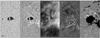 |
Fig. 1 Pore NOAA 11005, working FOV |
Horizontal motions of the intensity and Doppler structures in the working FOV were measured
by means of the method of local correlation tracking (LCT, November & Simon 1988). Applied to a time-series of images, LCT provides a
time-averaged horizontal velocity field of all the structures. We must keep in mind that
generally, such a velocity field does not always reflect the real flow of gas, for example,
in a penumbra (Sobotka 1999). On the other hand, flow
characteristics of photospheric granulation can be retrieved quite well by LCT (Verma et al. 2013). We used the filtered data, the FWHM
of the Gaussian tracking window was set to 1 2, and the
temporal integration was made over an interval of 52 min.
4. Chromospheric filamentary structure
4.1. Morphology
Examples of filtered intensity maps (WL, blue wing −60 pm from the line centre, and the Ca II 854.2 nm centre), a Ca II Doppler map and a LOS magnetogram are shown in Fig. 1. The magnetogram was calculated in arbitrary units by integrating the red lobe of the Fe I 617.3 nm V profile and the pore’s magnetic signal (black in Fig. 1e) was saturated at 15% of its maximum for better visualisation. Opposite-polarity patches (white) are clearly visible in the photosphere around the pore. In the Ca II wing we see the typical pattern of reverse granulation together with magnetic bright points. Short bright filaments surround the pore’s edge. These filaments are a manifestation of an inclined magnetic field that extends beyond the pore’s visible boundary in the form of spines (Sobotka et al. 2012).
In the line centre, the pore is surrounded by a filamentary structure composed of radially oriented bright and dark fibrils. This structure can be detected in the spectral range ±18 pm around the line centre. A similar structure is also seen in Doppler maps. The area and shape of the filamentary structure are identical in all pairs of the line-centre intensity and Doppler images in the time-series. It is expected that this structure is formed by magnetic field, extending into the chromosphere, which connects the pore with the observed photospheric patches of opposite magnetic polarity.
The fibrils begin immediately at the umbral border and in many cases continue to the
border of the filamentary structure. Their lengths are in the range
5′′−19′′ in the line centre and in the Doppler maps. Widths of the
fibrils were measured by means of power spectra calculated from intensity and Doppler
velocity variations along four quasi-circular curves perpendicular to the fibrils at
different distances from the pore. All power spectra are very similar each to other. They
do not show any particular peaks, instead, they decrease continuously until
0 5, where they
reach the noise level. This means that the fibrils do not have any typical width
detectable within the limits of our spatial resolution. The narrowest fibrils measured
directly in the best-quality intensity and Doppler images are
0 5 (3 pixels)
wide.
The fibrils seen in the Ca II line centre are spatially uncorrelated with those in the Doppler maps. This is similar to the situation in a superpenumbra of developed sunspots, where flow channels of the inverse Evershed effect are not identical with superpenumbral filaments (Tsiropoula et al. 1996). Thus, it is worth checking whether the inverse Evershed effect is also detectable in the filamentary structure around the pore.
4.2. Line-of-sight velocities
The statistical distribution of LOS velocities in the k–ω filtered series of Doppler maps, where everything except for the filamentary structure was masked out, is practically Gaussian, symmetric around zero, with σ = 0.40 km s-1. The minimum and maximum values are −2.5 and 4.7 km s-1, respectively. We adopted the sign convention where positive LOS velocities are directed away from the observer. The unfiltered LOS velocities, including oscillations and waves, also show a Gaussian distribution symmetric around zero, but its σ = 0.65 km s-1 is larger and the minimum-to-maximum range is [−3.4, 5.0] km s-1.
The filtered time-series of Doppler maps was averaged in time to obtain the spatial distribution of mean LOS velocities around the pore. The result is shown in Fig. 2 together with contours of −1, zero, and 1 km s-1. We can see from the figure that the inner part of the filamentary structure contains a positive LOS velocity (away from us, a downflow), while the outer part, located mostly on the limb side in the north, shows a negative LOS velocity (towards us, an upflow). Taking into account the heliocentric angle ϑ = 23° and assuming that the plasma moves along magnetic field lines that form a funnel, the negative LOS velocity is only partly generated by real upflows, but mostly by horizontal inflows into the pore. The picture of plasma moving towards the pore and flowing down in its vicinity is consistent with the inverse Evershed effect observed in the sunspots’ superpenumbra. This fact, together with the missing correlation between the fibrils observed in the line-centre and Doppler maps, leads us to the conclusion that the filamentary structure observed in the chromosphere above the pore is equivalent to a superpenumbra of a developed sunspot. The presence of running waves and a rapid change of oscillation frequencies at the boundary of the pore (see Sect. 5) further supports this inference.
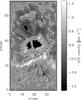 |
Fig. 2 Time-averaged Doppler map with contours of −1, zero, and 1 km s-1. The black dashed line outlines the border of the chromospheric filamentary structure around the pore. The arrow is directed towards the disc centre. |
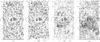 |
Fig. 3 Horizontal velocities of intensity and Doppler structures, integrated over a time interval of 52 min. From left to right: a) broad-band (WL) around 621 nm, b) Ca II 854.2 nm blue (−60 pm) wing, c) Ca II line centre, and d) Doppler structures. The black dashed line outlines the border of the chromospheric filamentary structure. The black bars at the beginning of the x-axis correspond to 1 km s-1 (note that their length is three times longer for (a),b) than for (c),d)). |
4.3. Horizontal velocities
Apparent horizontal motions of intensity and Doppler structures in the working FOV were measured using LCT (Sect. 3) in the filtered series of images. The resulting maps of horizontal velocities in WL, Ca II 854.2 nm blue (−60 pm) wing, Ca II line centre, and of Doppler structures are shown in Fig. 3. In the WL map we see a typical rosetta pattern of centres of diverging motions caused by repeated expansion and splitting of granules and commonly associated with mesogranules (e.g. Bonet et al. 2005, and references therein). The velocity magnitudes range from zero to 1.4 km s-1 with a mean value of 0.4 km s-1. Divergence centres just around the pore produce weak inflows of granules across the pore’s border, as was observed by Sobotka et al. (1999).
In the Ca II wing (Fig. 3b) we see a pattern similar to that in WL, which, in this case, describes horizontal motions in the reverse granulation. To our knowledge, such motions were never measured before. The velocity magnitudes are equal to and the divergence centres are approximately co-spatial with those in the WL granulation. The most important difference is that the inflows into the pore are absent. This can be explained by the fact that close to the pore’s border, the pattern of reverse granulation is replaced by short bright filaments (Sect. 4.1) that do not show any horizontal motions.
The typical apparent motion of chromospheric structures seen in the Ca II line centre and Doppler maps is directed radially away from the pore. The outflow area in the line centre is smaller than the area of the filamentary structure (Fig. 3c) and the spatial distribution of velocity magnitudes is irregular, with a maximum of 5–6 km s-1 (limited by the cutoff of the k–ω filter) south-west from the pore. The direction of the outflow is opposite to the real flow of gas, the inverse Evershed effect, derived from the LOS velocities. A visual inspection of movies composed of line-centre images reveals elongated diffuse bright and dark patches with sizes of 1′′−3′′ moving intermittently along the chromospheric fibrils away from the pore.
Motions of the Doppler structures (Fig. 3d) diverge from the centre of the large umbral core until 3′′–4′′ from the pore’s border with a typical speed of 3 km s-1. This type of motion is probably a residual of running waves (Sect. 5.2), the major part of which was removed by the k–ω filter. A strong outflow with an average speed 3 km s-1 and a maximum of 5−6 km s-1, observed in the region south of the pore, may be related to outward-moving patches with positive and negative LOS velocities – some of them are seen in Fig. 1d. A similar type of flocculent flows in the line Hα was described by Vissers & Rouppe van der Voort (2012).
Generally, the origin of the apparent horizontal outward motion of line-centre and Doppler structures is unclear. It might be caused by a combination of moving intensity or Doppler patches and residuals of running waves, but also by a spurious LCT correlation of chaotic transversal motions of fibrils.
5. Oscillations and waves
5.1. Observed oscillation properties
Before we began to analyse the oscillations in various magnetised regions, we performed a sanity check of the observations in the quiet-Sun regions. The spatial extent of quiet-Sun regions is large enough to construct standard helioseismic k − ω diagrams. We present them in Fig. 4, where we also overplot the eigenfrequencies of the first five ridges (f, p1 − p4) from Model S (Christensen-Dalsgaard et al. 1996) for reference. The left diagram, corresponding to the photosphere, is qualitatively similar to a k − ω diagram constructed from Helioseismic and Magnetic Imager (HMI; Scherrer et al. 2012; Schou et al. 2012) data, where we cropped the data cube in time and space to mimic the IBIS observations.
One can see from the figure that in the wings of the Ca II line (±54 pm from the line centre), where we analyse the signal of oscillations from the middle photosphere (h ≃ 200−300 km), individual ridges of solar oscillations can be identified, with the f mode clearly visible and some visibility of p1 and p2 modes. Higher-order p modes blend into a bulk in the k–ω diagram. An analogous diagram constructed for the centre of the line, thus representing the spatio-temporal behaviour of the intensity in the middle chromosphere (h ≃ 1300 km), is very different. The visibility of the acoustic ridges in the k–ω diagram drops rapidly because p modes do not propagate through the temperature minimum in the non-magnetised atmosphere. However, the power at those frequencies is not zero. This is probably a consequence of magneto-acoustic waves propagating through magnetic portals into the chromosphere. Stangalini et al. (2011) reported that magnetic fields are able to lower the cutoff frequency for acoustic waves, thus allowing the propagation of waves that would otherwise be trapped below the photosphere into the upper atmosphere. The power distribution averaged over the wave-number space resembles that displayed in Fig. 5 of Jefferies et al. (2006). It is also interesting to look at the spatial power distribution of plasma motions at frequencies lower than 2 mHz. In the middle chromosphere, the smaller scales have much less power, in contrast to the larger scales. This is not surprising, because the dynamics in the chromosphere must be completely different due to the lower density and dominance of the magnetic field.
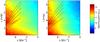 |
Fig. 4 Comparison of k–ω diagrams obtained for the quiet-Sun region, constructed for the wings of the Ca II line (left) and the centre of the line (right). Model S eigenfrequencies are overplotted with solid lines. |
The magnetised regions (the two umbral cores of the pore and the LB) have a very small spatial extent and an irregular shape, thus we do not discuss the corresponding k–ω diagram and focus on the properties of the power spectra in the frequency domain. The seismic properties of the pore are as expected from the literature and the eastern and western umbral cores have similar seismic properties.
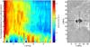 |
Fig. 5 Azimuthally averaged power spectra of the Ca II line-centre intensity as a function of the normalised radial distance from the pore’s centre and frequency (left) and a sketch of geometry used (right). The solid line encircles the safe boundary of the pore (see text). The radial distance is normalised with respect to this boundary (here R ≡ 1 for all angles). Two white dashed lines limit the angles used in the azimuthal average of the power spectra. The black dashed lines mark the cuts in x and y used to construct time-slice diagrams in Fig. 9. |
For a detailed study of the chromospheric power spectrum we selected the line-centre intensity in the larger eastern umbral core and analysed the change of the frequency power-spectrum as a function of the radial distance. The radial distance R was measured from the gravity centre of the umbral core (R = 0) and normalised at each azimuthal angle φ to the safe-boundary distance R = 1. This safe boundary was determined by hand from a time-averaged image in the Ca II wing (Fig. 5 right) and encircles the inner parts of the umbral core, excluding disturbances from the surroundings. We took into account only the directions pointing away from the LB, as shown in the figure. Then we averaged the frequency power spectra PI,centre(ν,R,φ) azimuthally over all points with the same normalised distance from the centre of the umbral core.
The result, plotted in Fig. 5 left, depicts dominant frequencies above 4 mHz in the umbra (R < 1.5), while outside the umbra (R > 1.5), all significant frequencies are below 5 mHz. There seems to be a systematic shift of the peak of the dominant frequency band for R < 1.5, with a power shifting towards lower frequencies when R increases – in agreement with the findings of Reznikova et al. (2012), suggesting the shift of the acoustic cut-off frequency with increasing inclination of the field lines. At R ~ 1.5 (the visible umbral boundary), the frequencies higher than 4 mHz essentially disappear from the power spectrum and all the power is shifted towards 2−3 mHz with a second power bulk at frequencies below 1 mHz, where plasma motions dominate. This is similar to the change in frequencies found by Tziotziou et al. (2007) at the penumbra-superpenumbra boundary (Fig. 6 of that paper). Therefore, the filamentary region around the pore depicts a seismic behaviour in the chromosphere similar to that of the superpenumbra of a sunspot.
It is interesting, however, to look at the seismic properties of the LB and compare them with the quiet Sun, because the magnetic-field strength is significantly lower in the LB than in the surrounding umbral cores of the pore. The power spectra averaged over all pixels belonging to the LB and quiet-Sun regions are displayed in Fig. 6. The power spectra of the LB are noisier because there forty times fewer pixels enter the averaging than in the quiet Sun. Interestingly, the power spectrum of the LB observed in the chromosphere is very similar to the photospheric power spectrum of the quiet Sun with a small drop of power below 2 mHz. To explain this observation, we suggest that the p modes, which are normally evanescent in the chromosphere, just leak into the chromosphere along the inclined magnetic field in the LB, which was also discussed by other authors (e.g., Cally 2006; De Pontieu et al. 2004). We assume that the lower frequency power is missing because although the LB has some properties similar to the solar photosphere, it is not the photosphere, and especially the convection is still operating in a degenerated state, which affects the conditions for the wave excitation.
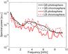 |
Fig. 6 Average power spectra of the quiet-Sun (QS) regions in the FOV constructed from the Ca II wings (photosphere) and the line centre (chromosphere), compared with the power spectra of the light bridge (LB) in the photosphere and chromosphere. |
From the time-series of Dopplergrams we constructed power maps for nine frequency bands around 1, 2, ..., 9 mHz with a transmission FWHM = 0.86 mHz. Six of these are displayed in Fig. 7. These power maps nicely show the changing spectral distribution of the acoustic emission. A region south of the pore is dominant in the low-frequency bands, which is probably an artefact caused by horizontal motions of Doppler structures (cf. Fig. 3d). The spectral power in frequency bands around 3 to 9 mHz is significantly lower in the filamentary region around the pore than in the surroundings. The acoustic emission in both umbral cores peaks around 5−7 mHz, that is, the band of three-minute oscillations. This agrees with Stangalini et al. (2012), who showed that the three-minute enhancement is strictly confined to the umbral region, while five-minute waves are suppressed here. Around 4 mHz, the power is dominant in the LB, a plage eastward of the pore, and at the edges of umbral cores. We assume that these are the regions where p modes leak up along the inclined magnetic field into the chromosphere.
5.2. Umbral flashes and running waves
Umbral flashes are seen in the Ca II 854.2 line core. They appear in the two umbral cores
of the pore and typically cover the whole area of each core. For a more detailed analysis
we selected a small 0 5 ×
0 5 area in the
centre of the dominant eastern umbral core and constructed a time vs. wavelength diagram
of temporal fluctuations of intensity in the observed Ca II line profile. This diagram,
together with fluctuations of the Doppler velocity visualised in a grey scale, is shown in
Fig. 8. We can see that umbral flashes appear as
intensity enhancements of chromospheric umbral oscillations and are connected with an
abrupt change from a redshift to a blueshift in the Doppler signal (Rouppe van der Voort et al. 2003).
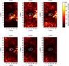 |
Fig. 7 Acoustic power maps measured from the series of Dopplergrams in six frequency bands around 2−7 mHz with FWHM of the transmission band 0.86 mHz. All panels have the same colour scale. |
Photospheric counterparts of umbral flashes are also seen in the Ca II line wings. From
the cross-correlation analysis we obtain that intensity brightenings in the ±54 pm wings
typically precede umbral flashes by 56 s. Assuming that umbral flashes are excited by
upward-propagating shock waves (Rouppe van der Voort et
al. 2003) and that the height difference between the formation levels of the Ca
II line wings and centre is 1000−1200 km, we obtain a mean phase-speed of the upward
propagation of approximately 20 km s-1. This speed is supersonic. The sound
speed 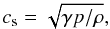 (1)where γ
is the adiabatic index equal to 5/3 for monoatomic gas, p is the gas
pressure, and ρ is the gas density, was estimated using the quiet-Sun
model VAL3C (Vernazza et al. 1981)
and the umbral model M (Maltby et al.
1986). In the middle photosphere, cs ≃ 7 and 6 km
s-1 for the quiet Sun and umbra, respectively, and in the middle
chromosphere, cs ≃ 8 and 9 km s-1.
(1)where γ
is the adiabatic index equal to 5/3 for monoatomic gas, p is the gas
pressure, and ρ is the gas density, was estimated using the quiet-Sun
model VAL3C (Vernazza et al. 1981)
and the umbral model M (Maltby et al.
1986). In the middle photosphere, cs ≃ 7 and 6 km
s-1 for the quiet Sun and umbra, respectively, and in the middle
chromosphere, cs ≃ 8 and 9 km s-1.
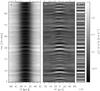 |
Fig. 8 Oscillations in the centre of the pore’s large umbral core. Prominent umbral flashes occur at t = 9, 29, and 32 min. a) Temporal fluctuations of intensity at different wavelengths in the Ca II line profile. b) Same as a) but enhanced by subtraction of the mean line profile. c) Visualised temporal fluctuations of the Doppler (LOS) velocity. Redshifts are bright. |
Concentric running waves originating in the centre of the dominant eastern umbral core and propagating beyond the pore’s edge into the chromospheric filamentary structure are observed in the unfiltered time-series of Ca II intensity and Doppler maps. In the intensity, the waves start to be detected in the line wings for | Δλ| < 30 pm, i.e., in the part of the line profile formed in the chromosphere. The waves are best observable in the line centre. The shapes of waves observed visually in pairs of line-centre intensity images and Dopplergrams are practically equal.
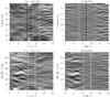 |
Fig. 9 Time-slices showing umbral flashes and running waves observed in difference maps (unfiltered − filtered) of the Ca II line-centre intensity (left) and Doppler velocity (right). The slices are constructed along the cuts in x (top) and y (bottom) directions displayed in Fig. 5. White lines mark edges of the umbra, black lines the borders of the light bridge. The grey scale of Doppler velocities ranges from −2 to 2 km s-1. |
To measure their speed and range of propagation, we used two time-series of difference maps of line-centre intensities and Doppler velocities, obtained by subtraction of the k–ω filtered images from the original ones. Then we constructed time-slice diagrams from two perpendicular cuts intersecting in the centre of the eastern umbral core (see Fig. 5, right). The time-slice diagrams are displayed in Fig. 9. Note the waves propagating through the smaller western umbral core (top left panel) and the strong Doppler velocity response in the LB with maximum amplitude ±4 km s-1 to umbral flashes (Fig. 9, top right). The mean phase velocity of running waves measured in the Ca II line-centre intensity is 9 km s-1, comparable to the sound speed in the chromosphere. The mean phase velocity derived from Dopplergrams is 10 km s-1. The waves pass the pore’s edge and propagate through the chromospheric filamentary structure to the distance of typically 3 Mm from the visible border of the pore, in extreme cases to 5−6 Mm, and then disappear. These waves are very similar to the running penumbral waves observed in the penumbral chromosphere and superpenumbrae of developed sunspots, described for instance by Christopoulou et al. (2000).
6. Light bridge
6.1. Structure and width
The strong granular LB separates the two umbral cores of the pore. It is the brightest feature inside the pore. In the chromosphere, it is by factor of 1.3 brighter than the average brightness in the working FOV. The granular structure of the LB is preserved at all heights, from the photospheric continuum level to the formation height of the Ca II line centre. It is interesting that while a typical pattern of reverse granulation, observed in the Ca II wings, appears outside the pore in the middle photosphere, the LB is always composed of small bright granules separated by dark intergranular lanes (see Fig. 1). This fact is discussed in Sect. 7.
A feature-tracking technique (Sobotka et al. 1997)
was applied to correlate the LB granules in position and time at different heights in the
atmosphere. A correlation was found between the photospheric LB granules in the WL and Ca
II wing (±60 pm) images with a correlation coefficient of 0.46. On the other hand, there
was no correlation between the chromospheric LB granules observed in the Ca II line centre
and the photospheric ones in the wings and continuum. The feature-tracking technique also
showed that the mean size of the LB granules increased with height from
0 45 in the WL
images to 0 50 in the Ca II
wings and 0 54 in the Ca II
line centre. Similarly, the average width of the LB increased with height in the
atmosphere from 2′′ (WL) to 2 5 (Ca II wings) and
3′′ (Ca II line centre). This contradicts the expectation that the width of
the LB magnetic structure decreases with height due to the presence of magnetic canopy.
To investigate the width of the LB at different heights in the photosphere, we used the
complementary HINODE observations in the two spectral lines Fe I 630.15 and 630.25 nm,
made 3 h 14 min before our observations started, and applied the inversion code SIR (see
Sect. 3) to retrieve vertical stratifications of
temperature and magnetic-field strength from the observed Stokes profiles. From the
resulting stratifications we created maps at five different optical depths from
τ500 = 0.004 to 1 with steps of
log (τ500) = 0.6. We cut across the central part of the LB
and measured the width of the structure in maps of temperature (corresponding to the
intensity at each height) and magnetic-field strength. The width was determined as a FWHM
related to the highest and lowest values in the cut. Since the HINODE pixel scale
0 3 is
insufficient to study the changes of LB width, we used the spline function to refine the
spatial sampling ten times. In Fig. 10 we present
changes of magnetic field strength and temperature along the cut through the pore and the
LB. Different curves correspond to five different optical depths. Dips in the temperature
profile of the LB at optical depths τ500 = 0.016−0.252
correspond to a central dark lane, seen also in the wings and centre of the Ca II line
(Fig. 1). The measured widths are summarised in Table
1 together with geometrical heights and lowest
values of the magnetic-field strength in the LB, obtained from the inversions.
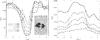 |
Fig. 10 Profiles of magnetic-field strength B (left) and temperature T (right) across the light bridge at different optical depths τ500, obtained by inverting HINODE observations. The location of the cut is shown in the inset. Crosses denote data points obtained by the inversion code and black squares the positions used to measure the width. |
Widths of the light bridge measured from temperature and magnetic field maps (HINODE observations) at different optical depths τ500 in the photosphere.
The width of the LB in temperature in the low photosphere is approximately constant
(2 7). At higher
layers, the LB becomes wider. However, at the highest studied optical depth, the
temperature contrast between the pore and the LB is low, which results in a higher error
of the measured width. The temperature response functions are also close to zero at this
optical depth, that is, the retrieved temperature values have higher uncertainties than
deeper photospheric layers. On the other hand, the LB is becoming narrower with height in
the maps of the magnetic-field strength B. This corresponds to the
magnetic canopy above the LB, which was observationally confirmed by Jurčák et al. (2006). The magnetic field from the surrounding umbral
cores is expanding above the LB’s weaker field, forming a cusp-like structure at the
height h ≃ 220 km (Giordano et al.
2008). Note that the central part of the LB is almost field-free at the lowest
photospheric layer. However, the response function to B is close to zero
there and the retrieved values of B have high errors (±250 G). At the
highest optical depth, the uncertainties of B are also of this order. The
errors at other optical depths are typically ±100 G.
As a whole, the LB centre is shifting towards the smaller umbral core (see Fig. 10). This is caused by the more inclined magnetic field in the large eastern umbral core, which expands faster above the LB than the almost vertical magnetic field from the smaller core. In Sobotka et al. (2012) we determined the magnetic-field inclination and azimuth in the LB from inversions of Stokes profiles of Fe I 617.33 nm, observed simultaneously with the Ca II line. The azimuth direction is perpendicular to the LB axis. The magnetic-field inclination is 30°−35°, measured at τ500 = 0.03−0.1, which corresponds to the height h of about 100 km, that is, below the cusp height. For the oscillation propagation the inclination above the cusp height is important, which is composed of the 10° general tilt of the pore’s field (Sect. 2) and the inclination of the dominant expanding field of the large umbral core, extrapolated to high photosphere (h > 400 km). We made this extrapolation using straight field lines and obtained a total inclination of 40°−45°. If the curvature of extrapolated field lines is taken into account, the inclination can reach 50°.
6.2. Acoustic flux
From the preceding section it becomes clear that the apparent width of the LB is larger than the width of the structure with reduced magnetic field within the LB. At the same time, the LB in the chromosphere is by factor of 1.3 brighter than the average brightness in the FOV. Therefore, there must be some heating mechanism to explain these observed properties. Oscillations are detected both in the photosphere and chromosphere, so that we estimated the amount of energy transferred by oscillations from the photosphere to the higher atmosphere.
Following Bello González et al. (2009), we
estimated from the Doppler velocities the acoustic energy flux in the chromosphere of the
LB and compared it with the flux in the quiet chromosphere. The method of power spectra
calculation and calibration in absolute units is described by Rieutord et al. (2010). It is evident from the power maps in Fig. 7 that in the region of the LB, the oscillatory power at
frequencies different from both umbra and quiet chromosphere dominates, while it is
similar in behaviour to the plage region eastward of the pore. The acoustic power flux can
be estimated from the equation 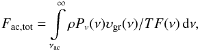 (2)where
Pv is the velocity spectral power density,
υgr is the group velocity with which the energy is
transported, given by
(2)where
Pv is the velocity spectral power density,
υgr is the group velocity with which the energy is
transported, given by  (3)cs
is the sound speed from Eq. (1) and νac is the acoustic cutoff
frequency given by
(3)cs
is the sound speed from Eq. (1) and νac is the acoustic cutoff
frequency given by  (4)with g
being the surface gravity and θ the magnetic field inclination. The
effect of magnetic-field inclination that lowers the acoustic cutoff frequency was
analytically derived by Cally (2006).
(4)with g
being the surface gravity and θ the magnetic field inclination. The
effect of magnetic-field inclination that lowers the acoustic cutoff frequency was
analytically derived by Cally (2006).
For the model atmosphere used to derive the acoustic cutoff and group velocity we adopted the values of ρ = 6.5 × 10⁻⁸ kg m-3 and p = 2.5 Pa from the VAL3C model (Vernazza et al. 1981) averaged over heights of 900−1200 km. We expect that this model of an average quiet chromosphere also provides reasonable values for the LB. We estimated the field inclination θ = 50° by extrapolating the inversion results (Sect. 6.1) obtained for the photospheric layers.
The function TF(ν) in the equation given above denotes the transfer function of the solar atmosphere. The extent in atmospheric heights of the spectral-line contribution function decreases the observable signal of small-scale fluctuations along the LOS, thus the signal with shorter periods is usually retrieved by observations with decreased power. For the estimate in this paper we did not attempt to derive the correct TF and set TF(ν) = 1 for all frequencies. The correction using the transfer function may increase the total estimated power by a factor of two or similar, which, given the other assumptions we made, is not critical in our estimate.
The spectral power density Pv(ν) was derived from the series of Dopplergrams computed in the inner wings of the spectral line with the assumed height in the atmosphere around 1000 km. In the map we then segmented out the region of the LB and also the region of the quiet chromosphere for comparison (Fig. 11). The total acoustic power flux averaged over the LB region measured using our assumptions is 3400 W m-2, while only 680 W m-2 in the quiet-chromosphere region. One can easily note that the peak acoustic flux within the LB reaches values as high as 10 000 W m-2 averaged over an observation pixel. These peak values are much higher than the value of 1840 W m-2 reported by Bello González et al. (2009), obtained for the quiet photosphere for uncorrected data, that is, with TF(ν) = 1. It seems that in the quiet-Sun regions, some of the acoustic flux of the p modes is transferred to the chromosphere, possibly along the inclined magnetic field at supergranular boundaries. However, in the studied LB and similarly in the plage region (see Fig. 11) the p-mode power flux into the active chromosphere is much higher and probably contributes to the plasma heating in these regions.
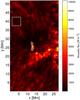 |
Fig. 11 Map of the total acoustic power flux with the selection of the light-bridge region and the region of the quiet chromosphere (square). |
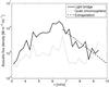 |
Fig. 12 Frequency distribution of the spatially averaged acoustic power flux in the light bridge and the quiet chromosphere. |
Again following Bello González et al. (2009), we extrapolated the high-frequency tail of the Pv(ν) using a power law to account for acoustic flux caused by the high-frequency waves (Fig. 12). The correction is very small however. Taking the estimated tail contribution into account, the total spatially averaged acoustic flux is 3460 W m-2, thus the extrapolated tail adds only a negligible 2% of the flux.
We note that the estimate of the acoustic power might be biased because of the inaccuracies in the modelling. For example, the map of the acoustic flux in Fig. 11 was computed assuming the VAL3C atmosphere at each pixel, which certainly is inappropriate. We did not attempt to appropriately model the atmosphere in each pixel of the map, since we have measurements only in one spectral line. However, to investigate the sensitivity of the derived acoustic flux to atmospheric parameters we repeated the calculations using a set of semi-empirical atmospheric models (VAL3A, VAL3B, VAL3C, Maltby-M). The resulting numbers vary by as much as 30%, which we estimate to be the level of our uncertainty. Another uncertainty comes from the unknown transfer function TF of the solar atmosphere, to derive which, a detailed time-dependent model of the atmosphere is needed. Note that incorporating the correct transfer function increases the estimate for the acoustic power flux. Bello González et al. (2009) found a correcting factor of 1.7 for a photospheric spectral line. Accordingly, our numbers should be seen as qualitative estimates – the real acoustic power flux may be a factor of a few different from our numbers, probably larger. Our intention is just to compare the acoustic flux in the LB with the surrounding quiet chromosphere to shed some light on the heat dissipation process observed in the LB chromosphere.
6.3. Radiative losses
To investigate whether the acoustic flux along the inclined magnetic field above the LB
might be responsible for the heating of the plasma within the LB chromosphere and
consequently for the increased optical width of the LB, we estimated the radiative losses
and compared them with the estimated heat deposited by the waves. We evaluated the
equation ![\begin{equation} \nabla \cdot \left[ F_{\rm ac,tot} + F_{\rm other} \right] = Q, \label{eq:heatballance} \end{equation}](/articles/aa/full_html/2013/12/aa22148-13/aa22148-13-eq102.png) (5)where
Fac,tot is the acoustic power flux computed
from Eq. (2),
Fother is the power flux from other sources, such as
small-scale reconnections (Shimizu 2012), and
Q are the radiative losses (net radiative cooling rates).
(5)where
Fac,tot is the acoustic power flux computed
from Eq. (2),
Fother is the power flux from other sources, such as
small-scale reconnections (Shimizu 2012), and
Q are the radiative losses (net radiative cooling rates).
To consider the radiative losses, we made a rough estimate based on the standard semi-empirical models by Vernazza et al. (1981) that fit our Ca II profiles quite well. The observed line profiles, averaged in time over the whole observing period and spatially over the LB and quiet-chromosphere regions marked in Fig. 11, were normalised to the atlas profile (Linsky et al. 1970) using the far wings of the line, where both observed profiles coincide. As evident from Fig. 13, the spatially averaged profiles may be reasonably fitted with the VAL3C model in the LB, and VAL3A or VAL3B models in the quiet chromosphere (from now on we use the VAL3B model of the average intranetwork area). It is well known that the computed Ca II line profiles are very sensitive to values of the microturbulent velocity. Higher microturbulence smoothes the small humps in the near wings, while zero microturbulence leads to a large enhancement of them; these results are consistent with the Ca II modelling by Uitenbroek (1989). Since we do not know the realistic distribution of microturbulent velocities in the LB, which can also be related to the acoustic-wave dynamics, we just used the standard VAL3C distribution. Our computed profile, when convolved with an instrumental or macroturbulent broadening, can give even a better fit to the observed LB profile than that shown in Fig. 13.
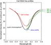 |
Fig. 13 Profiles of line Ca II 854.2 nm. The observed profiles in the light bridge (red) and quiet chromosphere (black) are averaged in time and over the corresponding areas marked in Fig. 11 and are normalised to the atlas profile (blue dashes) in the line wing. Green lines show profiles calculated using the models VAL3A, B, and C. |
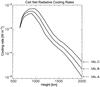 |
Fig. 14 Ca II net radiative cooling rates vs. geometrical height, calculated for the models VAL3A, B, and C. |
The Ca II line profiles and radiative losses were computed for the three VAL models, using a non-LTE atmospheric code based on the MALI technique (Rybicki & Hummer 1991, 1992), with standard partial frequency redistribution (PRD, angle-averaged) in the CaII H and K resonance lines. The hydrogen version of the code (with PRD in Lyman lines) first computes the ionisation structure and hydrogen level populations, then the Ca II version is used with a five-level plus continuum atomic model. In the range of heights of interest, the hydrogen losses were found to be much smaller than the Ca II ones. The Ca II losses in the H and K lines and in the infrared triplet, integrated over heights, agree with those computed by Vernazza et al. (1981) using a similar PRD approach. For the model VAL3C, these authors also provided integrated losses in the Mg II h and k lines, which amount roughly to one third of the Ca II losses. We use this estimate in our Table 3. The Ca II net radiative cooling rates are plotted in Fig. 14 and the total Ca II radiative losses, that is, the net cooling rates integrated over all heights displayed in the figure, are given in Table 2. Note that the dominant contribution of the integral comes from the heights 700−1400 km; outside of this interval, the contribution is an order of magnitude smaller.
The acoustic flux was estimated at two heights in the chromosphere: at
h ~ 1000 km from the series of Dopplergrams measured in the inner wings
of the line by the double-slit method, and at h ~ 1400 km from the
Dopplergrams obtained by the parabolic fit of the line centre. Hence, by integrating Eq.
(5) over height h and
neglecting the horizontal variations of the energy flux, as we deal with the spatially
averaged values, we obtain ![\begin{eqnarray} \label{eq:heatintegrated} && \int_{h_1}^{h_2} \frac{{\rm d} \left[F_{\rm ac,tot} + F_{\rm other}\right]}{{\rm d}h}\,{\rm d}h = \nonumber\\ && F_{\rm ac,tot}(h_2) - F_{\rm ac,tot}(h_1) + \Delta F_{\rm other} = \int Q\,{\rm d}h \equiv Q_{\rm tot}, \end{eqnarray}](/articles/aa/full_html/2013/12/aa22148-13/aa22148-13-eq108.png) (6)where
h1 = 1000 km, h2 = 1400 km, and
we ignored the contribution of other energy sources ΔFother.
The acoustic fluxes were calculated using densities and gas pressures from the models
VAL3C for the LB and VAL3B for the quiet chromosphere.
A magnetic field inclined by 50° was assumed in the LB. The estimated values of
acoustic fluxes and radiative losses of Ca II + Mg II are summarised in Table 3.
(6)where
h1 = 1000 km, h2 = 1400 km, and
we ignored the contribution of other energy sources ΔFother.
The acoustic fluxes were calculated using densities and gas pressures from the models
VAL3C for the LB and VAL3B for the quiet chromosphere.
A magnetic field inclined by 50° was assumed in the LB. The estimated values of
acoustic fluxes and radiative losses of Ca II + Mg II are summarised in Table 3.
Total radiative losses Qtot of Ca II integrated over geometrical heights 600−2000 km.
Acoustic power fluxes Fac,tot at geometrical heights h1 = 1000 km and h2 = 1400 km, their difference ΔFac,tot, and an estimate Qtot of total radiative losses of Ca II and Mg II.
Taking into account that the error level in the determination of the total acoustic flux may be of the order of tens of per cent and the obtained values are probably underestimated (see Sect. 6.2), one has to look at the numbers more qualitatively. The calculated radiative cooling in the quiet chromosphere is very probably overestimated – as we mentioned, the profile of the Ca II line corresponds to a model cooler than VAL3B, between VAL3A and VAL3B. It is evident that in the quiet chromosphere, the p modes leaking along the small-scale magnetic fields are not important for the heating of the plasma and the term ΔFother dominates the left-hand side of Eq. (6). However, in the chromosphere above the LB, the increased heating by p modes leaking along the inclined magnetic field practically fully explains the excess in plasma radiation. To verify this claim, detailed time-dependent MHD and radiative-transfer models are needed.
7. Discussion and conclusions
We studied the photosphere and chromosphere of a large solar pore with a granular LB using
spectral-imaging observations in the line Ca II 854.2 nm and complementary
spectropolarimetric observations in photospheric lines of Fe I. Dopplergrams mapping
chromospheric LOS velocities at the height of approximately 1000 km were derived from the Ca
II line core and power maps of acoustic oscillations were calculated for frequency bands
around 1−9 mHz. The spatial resolution was approximately
0 4.
We showed that the chromospheric filamentary structure around the pore, observed in the Ca II line core and Doppler maps, has all the important characteristics of a superpenumbra. It is composed of radially oriented fibrils, which are spatially uncorrelated with the fibrils seen in the Dopplergrams. The spatial distribution of time-averaged LOS velocities corresponds to the inverse Evershed effect. Concentric running waves propagate through the filamentary structure with the speed of sound and the observed characteristics of acoustic oscillations correspond to those in a superpenumbra. Although a strong horizontal magnetic field responsible for the formation of a penumbra is missing in the pore, the magnetic field of B ≃ 1500 G at the pore’s border inclined by 40° (Sobotka et al. 2012) manifests itself in the middle photosphere by short bright filaments seen in the Ca II line wings (Fig. 1b) and its field lines, which return to opposite-polarity patches dispersed in the photosphere around the pore, very probably form the filamentary structure with superpenumbral characteristics in the chromosphere. From this point of view, the presence of a penumbra is not a necessary condition for the formation of a superpenumbra.
Horizontal motions of photospheric structures around the pore were measured using the LCT method at two different heights: h ≃ 0 km (continuum images around 621 nm) and h ≃ 250 km (images in Ca II blue wing −60 pm), where the reverse granulation is observed. We found that horizontal flows with typical centres of diverging motions, corresponding to mesogranules, are identical at both heights. LCT measurements in the Ca II line centre images and Dopplergrams, that is, in the middle chromosphere, reveal radial motions away from the pore that are located inside the superpenumbra. Their origin is not clear yet and needs additional investigation.
Umbral flashes observed in both cores of the pore seem to be excited by shock waves (cf. Rouppe van der Voort et al. 2003) that propagate upwards with a supersonic speed of 20 km s-1. An enhanced power of acoustic oscillations at frequencies around 3−5 mHz was observed in the LB inside the pore, in a plage eastward of the pore, and at the edges of umbral cores. We assume that these are the regions where acoustic waves leak up along the inclined magnetic field into the chromosphere, as predicted by De Pontieu et al. (2004) and Cally (2006).
Special attention was paid to the granular LB that separated the pore into two umbral cores. Its width measured in magnetic field maps decreases with increasing height in the atmosphere, which confirms the magnetic canopy structure (Jurčák et al. 2006). On the other hand, the width measured in intensity and temperature maps increases with height as well as the size of LB granules.
In the middle photosphere (h ≃ 250 km, Ca II wings), reverse granulation is seen around the pore, but not in the LB. The reverse granulation is explained by adiabatic cooling of expanding gas in granules, which is only partially cancelled by radiative heating (Cheung et al. 2007). In the LB, hot magnetoconvective plumes at the bottom of the photosphere cannot expand adiabatically in higher photospheric layers because of the magnetic field and the radiative heating dominates, forming small bright granules separated by dark lanes. The positive correlation between the LB structures in the continuum and Ca II line wings indicates that the middle-photosphere structures are heated by radiation from the low photosphere. Since the mean free photon path in the photosphere is longer than 1′′ for h > 120 km, the LB observed in the line wings is broader and its granules are larger than in the continuum due to the radiation diffusion.
In the middle chromosphere (h ≃ 1300 km, Ca II centre), the LB is the brightest feature in the pore and it is brighter by factor of 1.3 than the average intensity in the FOV. Since the height in the atmosphere is well above the temperature minimum, radiative heating cannot be expected. The heating by acoustic waves seems to be a candidate, because the measured acoustic power flux in the LB is five to seven times higher than that in the quiet chromosphere. This is because p modes leak along the inclined magnetic field in the LB and propagate into the chromosphere. To investigate this possibility, we compared the acoustic power flux with total radiative losses and found that the acoustic power flux dissipation in the LB, estimated to 3000 W m-2 as a minimum, can indeed account quite well for the total radiative losses (4300 W m-2) computed using the VAL3C model, which fits our observed CaII 854.2 nm line profile in the LB.
However, this profile is averaged in time and over the LB area, which may have certain consequences for the modelling. As is now well established from radiation-hydrodynamical simulations of the solar chromosphere (e.g., Carlsson & Stein 1998), semi-empirical models based on time-averaged line profiles generally overestimate the true mean temperature, especially in the UV, where the line-intensity averaging is highly nonlinear. Therefore our computed radiative losses based on this enhanced empirical temperature and density distribution have to be considered with caution. It may be that the acoustic waves do not lead to an enhancement of the mean chromospheric temperature, but rather cause episodic brightenings within the acoustic shocks, where the wave energy converts almost instantaneously into radiation – this is at least the case of the quiescent chromosphere in the cell interior (Carlsson & Stein 1998). Therefore, to confirm our conclusions about the wave heating, detailed time-dependent simulations are needed.
Acknowledgments
We thank Marta Vantaggiato for her participation in the observations. This work was supported by the Czech Science Foundation under grants P209/12/0287 and P209/12/P568 and by the project RVO:67985815 of the Academy of Sciences of the Czech Republic. The Dunn Solar Telescope is located at the National Solar Observatory, which is operated by the Association of Universities for Research in Astronomy, Inc. (AURA), for the National Science Foundation. IBIS has been built by INAF/Osservatorio Astrofisico di Arcetri with contributions from the Universities of Firenze and Roma “Tor Vergata”, the National Solar Observatory, and the Italian Ministries of Research (MIUR) and Foreign Affairs (MAE). HINODE is a Japanese mission developed and launched by ISAS/JAXA, with NAOJ as domestic partner and NASA and STFC (UK) as international partners. It is operated by these agencies in cooperation with ESA and NSC (Norway).
References
- Alissandrakis, C. E., Dialetis, D., Mein, P., Schmieder, B., & Simon, G. 1988, A&A, 201, 339 [NASA ADS] [Google Scholar]
- Beckers, J. M., & Schröter, E. H. 1969, Sol. Phys., 10, 384 [NASA ADS] [CrossRef] [Google Scholar]
- Beckers, J. M., & Schultz, R. B. 1972, Sol. Phys., 27, 61 [NASA ADS] [CrossRef] [Google Scholar]
- Beckers, J. M., & Tallant, P. E. 1969, Sol. Phys., 7, 351 [NASA ADS] [CrossRef] [MathSciNet] [Google Scholar]
- Bello González, N., Flores Soriano, M., Kneer, F., & Okunev, O. 2009, A&A, 508, 941 [NASA ADS] [CrossRef] [EDP Sciences] [Google Scholar]
- Berger, T. E., & Berdyugina, S. V. 2003, ApJ, 589, L117 [NASA ADS] [CrossRef] [Google Scholar]
- Bhatnagar, A., Livingston, W. C., & Harvey, J. W. 1972, Sol. Phys., 27, 80 [NASA ADS] [CrossRef] [Google Scholar]
- Bogdan, T. J., & Judge, P. G. 2006, Phil. Trans. R. Soc. London, Ser. A, 364, 313 [Google Scholar]
- Bonet, J. A., Márquez, I., Muller, R., Sobotka, M., & Roudier, Th. 2005, A&A, 430, 1089 [NASA ADS] [CrossRef] [EDP Sciences] [Google Scholar]
- Brynildsen, N., Maltby, P., Leifsen, T., et al. 1999, Sol. Phys., 191, 129 [NASA ADS] [CrossRef] [Google Scholar]
- Cally, P. S. 2006, Phil. Trans. Soc. London Ser. A, 364, 333 [Google Scholar]
- Carlsson, M., & Stein, R. F. 1998, in New eyes to see inside sun and stars, eds. F.-L. Deubner, J. Christensen-Dalsgaard, & D. Kurtz, IAU Symp., 185, 435 [Google Scholar]
- Cauzzi, G., Reardon, K. P., Uitenbroek, H., et al. 2008, A&A, 480, 515 [NASA ADS] [CrossRef] [EDP Sciences] [Google Scholar]
- Cavallini, F. 2006, Sol. Phys., 236, 415 [NASA ADS] [CrossRef] [Google Scholar]
- Cheung, M. C. M., Schüssler, M., & Moreno Insertis, F. 2007, A&A, 461, 1163 [NASA ADS] [CrossRef] [EDP Sciences] [Google Scholar]
- Christensen-Dalsgaard, J., Dappen, W., Ajukov, S. V., et al. 1996, Science, 272, 1286 [CrossRef] [Google Scholar]
- Christopoulou, E. B., Georgakilas, A. A., & Koutchmy, S. 2000, A&A, 354, 305 [NASA ADS] [Google Scholar]
- De Pontieu, B., Erdélyi, R., & James, S. P. 2004, Nature, 430, 536 [NASA ADS] [CrossRef] [PubMed] [Google Scholar]
- Garcia, A., Klvaňa, M., & Sobotka, M. 2010, Cent. Eur. Astrophys. Bull., 34, 47 [NASA ADS] [Google Scholar]
- Giordano, S., Berrilli, F., Del Moro, D., & Penza, V. 2008, A&A, 489, 747 [NASA ADS] [CrossRef] [EDP Sciences] [Google Scholar]
- Giovanelli, R. G. 1972, Sol. Phys., 27, 71 [NASA ADS] [CrossRef] [Google Scholar]
- Hirzberger, J. 2003, A&A, 405, 331 [NASA ADS] [CrossRef] [EDP Sciences] [Google Scholar]
- Jefferies, S. M., McIntosh, S. W., Armstrong, J. D., et al. 2006, ApJ, 648, L151 [Google Scholar]
- Jurčák, J., Martínez Pillet, V., & Sobotka, M. 2006, A&A, 453, 1079 [NASA ADS] [CrossRef] [EDP Sciences] [Google Scholar]
- Keil, S. L., Balasubramaniam, K. S., Smaldone, L. A., & Reger, B. 1999, ApJ, 510, 422 [NASA ADS] [CrossRef] [Google Scholar]
- Keppens, R., & Martínez Pillet, V. 1996, A&A, 316, 229 [NASA ADS] [Google Scholar]
- Khomenko, E., & Cally, P. S. 2012, ApJ, 746, 68 [NASA ADS] [CrossRef] [Google Scholar]
- Klimchuk, J. A. 2006, Sol. Phys., 234, 41 [NASA ADS] [CrossRef] [Google Scholar]
- Kosugi, T., Matsuzaki, K., Sakao, T., et al. 2007, Sol. Phys., 243, 3 [NASA ADS] [CrossRef] [Google Scholar]
- Leka, K. D. 1997, ApJ, 484, 900 [NASA ADS] [CrossRef] [Google Scholar]
- Linsky, J. F., Teske, R. G., & Wilkinson, C. W. 1970, Sol. Phys., 11, 374 [NASA ADS] [CrossRef] [Google Scholar]
- Lites, B. W. 1992, in Sunspots: theory and observations, eds. J. H. Thomas, & N. O. Weiss, Proc. NATO ASI Series, C375 (Dordrecht: Kluwer), 261 [Google Scholar]
- Lites, B. W., Bida, T. A., Johannesson, A., & Scharmer, G. B. 1991, ApJ, 373, 683 [NASA ADS] [CrossRef] [Google Scholar]
- Maltby, P., Avrett, E. H., Carlsson, M., et al. 1986, ApJ, 306, 284 [Google Scholar]
- November, L. J., & Simon, G. W. 1988, ApJ, 333, 427 [Google Scholar]
- Ortiz, A., Bellot Rubio, L. R., & Rouppe van der Voort, L. 2010, ApJ, 713, 1282 [NASA ADS] [CrossRef] [Google Scholar]
- Reardon, K. P., & Cavallini, F. 2008, A&A, 481, 897 [NASA ADS] [CrossRef] [EDP Sciences] [Google Scholar]
- Reznikova, V. E., Shibasaki, K., Sych, R. A., & Nakariakov, V. M. 2012, ApJ, 746, 119 [NASA ADS] [CrossRef] [Google Scholar]
- Rieutord, M., Roudier, T., Rincon, F., et al. 2010, A&A, 512, A4 [NASA ADS] [CrossRef] [EDP Sciences] [Google Scholar]
- Rimmele, T. R. 1997, ApJ, 490, 458 [NASA ADS] [CrossRef] [Google Scholar]
- Rimmele, T. R., Richards, K. Hegwer, S., et al. 2009, in Telescopes and instrumentation for solar astrophysics, eds. S. Fineschi, & M. A. Gummin, Proc. SPIE, 5171, 179 [Google Scholar]
- Rouppe van der Voort, L. H. M., Rutten, R. J., Sütterlin, P., et al. 2003, A&A, 403, 277 [NASA ADS] [CrossRef] [EDP Sciences] [Google Scholar]
- Rucklidge, A. M., Schmidt, H. U., & Weiss, N. O. 1995, MNRAS, 273, 491 [NASA ADS] [CrossRef] [Google Scholar]
- Ruiz Cobo, B., & del Toro Iniesta, J. C. 1992, ApJ, 398, 375 [NASA ADS] [CrossRef] [Google Scholar]
- Rüedi, I., Solanki, S. K., & Livingston, W. 1995, A&A, 302, 543 [NASA ADS] [Google Scholar]
- Rybicki, G. B., & Hummer, D. G. 1991, A&A, 245, 171 [NASA ADS] [Google Scholar]
- Rybicki, G. B., & Hummer, D. G. 1992, A&A, 262, 209 [NASA ADS] [Google Scholar]
- Scherrer, P. H., Schou, J., Bush, R. I., et al. 2012, Sol. Phys., 275, 207 [Google Scholar]
- Schou, J., Scherrer, P. H., Bush, R. I., et al. 2012, Sol. Phys., 275, 229 [Google Scholar]
- Shimizu, T. 2012, in Hinode-3: The 3rd Hinode science meeting, eds. T. Sekii, T. Watanabe, & T. Sakurai, ASP Conf. Ser., 454, 177 [Google Scholar]
- Simon, G. W., & Weiss, N. O. 1970, Sol. Phys., 13, 85 [NASA ADS] [CrossRef] [Google Scholar]
- Sobotka, M. 1999, in Motions in the solar atmosphere, eds. A. Hanslmeier, & M. Messerotti (Dordrecht: Kluwer), 71 [Google Scholar]
- Sobotka, M., & Jurčák, J. 2009, ApJ, 694, 1080 [NASA ADS] [CrossRef] [Google Scholar]
- Sobotka, M., Brandt, P. N., & Simon, G. W. 1997, A&A, 328, 682 [NASA ADS] [Google Scholar]
- Sobotka, M., Vázquez, M., Bonet, J. A., Hanslmeier, A., & Hirzberger, J. 1999, ApJ, 511, 436 [NASA ADS] [CrossRef] [Google Scholar]
- Sobotka, M., Del Moro, D., Jurčák, J., & Berrilli, F. 2012, A&A, 537, A85 [NASA ADS] [CrossRef] [EDP Sciences] [Google Scholar]
- Stangalini, M., Del Moro, D., Berrilli, F., & Jefferies, S. M. 2011, A&A, 534, A65 [NASA ADS] [CrossRef] [EDP Sciences] [Google Scholar]
- Stangalini, M., Giannattasio, F., Del Moro, D., & Berrilli, F. 2012, A&A, 539, L4 [NASA ADS] [CrossRef] [EDP Sciences] [Google Scholar]
- Sütterlin, P. 1998, A&A, 333, 305 [NASA ADS] [Google Scholar]
- Thomas, J. H., & Weiss, N. O. 2008, Sunspots and Starspots (Cambridge University Press) [Google Scholar]
- Tsiropoula, G., Alissandrakis, C. E., Dialetis, D., & Mein, P. 1996, Sol. Phys., 167, 79 [Google Scholar]
- Tsuneta, S., Ichimoto, K., Katsukawa, Y., et al. 2008, Sol. Phys., 249, 167 [NASA ADS] [CrossRef] [Google Scholar]
- Tziotziou, K., Tsiropoula, G., Mein, N., & Mein, P. 2006, A&A, 456, 689 [NASA ADS] [CrossRef] [EDP Sciences] [Google Scholar]
- Tziotziou, K., Tsiropoula, G., Mein, N., & Mein, P. 2007, A&A, 463, 1153 [NASA ADS] [CrossRef] [EDP Sciences] [Google Scholar]
- Uitenbroek, H. 1989, A&A, 213, 360 [NASA ADS] [Google Scholar]
- van Noort, M., Rouppe van der Voort, L., & Löfdahl, M. 2006, in Solar MHD theory and observations, eds. J. Leibacher, R. F. Stein, & H. Uitenbroek, ASP Conf. Ser., 354, 55 [Google Scholar]
- Verma, M., Steffen, M., Denker, C. 2013, A&A, 555, A136 [NASA ADS] [CrossRef] [EDP Sciences] [Google Scholar]
- Vernazza, J. E., Avrett, E. H., & Loeser, R. 1981, ApJS, 45, 635 [NASA ADS] [CrossRef] [Google Scholar]
- Vissers, G., & Rouppe van der Voort, L. 2012, ApJ, 750, 22 [NASA ADS] [CrossRef] [Google Scholar]
- Viticchié, B., Del Moro, D., Criscuoli, S., & Berrilli, F. 2010 ApJ, 723, 787 [Google Scholar]
- Zirin, H., & Stein, A. 1972, ApJ, 178, L85 [NASA ADS] [CrossRef] [Google Scholar]
All Tables
Widths of the light bridge measured from temperature and magnetic field maps (HINODE observations) at different optical depths τ500 in the photosphere.
Total radiative losses Qtot of Ca II integrated over geometrical heights 600−2000 km.
Acoustic power fluxes Fac,tot at geometrical heights h1 = 1000 km and h2 = 1400 km, their difference ΔFac,tot, and an estimate Qtot of total radiative losses of Ca II and Mg II.
All Figures
|
Fig. 1 Pore NOAA 11005, working FOV |
| In the text | |
|
Fig. 2 Time-averaged Doppler map with contours of −1, zero, and 1 km s-1. The black dashed line outlines the border of the chromospheric filamentary structure around the pore. The arrow is directed towards the disc centre. |
| In the text | |
|
Fig. 3 Horizontal velocities of intensity and Doppler structures, integrated over a time interval of 52 min. From left to right: a) broad-band (WL) around 621 nm, b) Ca II 854.2 nm blue (−60 pm) wing, c) Ca II line centre, and d) Doppler structures. The black dashed line outlines the border of the chromospheric filamentary structure. The black bars at the beginning of the x-axis correspond to 1 km s-1 (note that their length is three times longer for (a),b) than for (c),d)). |
| In the text | |
|
Fig. 4 Comparison of k–ω diagrams obtained for the quiet-Sun region, constructed for the wings of the Ca II line (left) and the centre of the line (right). Model S eigenfrequencies are overplotted with solid lines. |
| In the text | |
|
Fig. 5 Azimuthally averaged power spectra of the Ca II line-centre intensity as a function of the normalised radial distance from the pore’s centre and frequency (left) and a sketch of geometry used (right). The solid line encircles the safe boundary of the pore (see text). The radial distance is normalised with respect to this boundary (here R ≡ 1 for all angles). Two white dashed lines limit the angles used in the azimuthal average of the power spectra. The black dashed lines mark the cuts in x and y used to construct time-slice diagrams in Fig. 9. |
| In the text | |
|
Fig. 6 Average power spectra of the quiet-Sun (QS) regions in the FOV constructed from the Ca II wings (photosphere) and the line centre (chromosphere), compared with the power spectra of the light bridge (LB) in the photosphere and chromosphere. |
| In the text | |
|
Fig. 7 Acoustic power maps measured from the series of Dopplergrams in six frequency bands around 2−7 mHz with FWHM of the transmission band 0.86 mHz. All panels have the same colour scale. |
| In the text | |
|
Fig. 8 Oscillations in the centre of the pore’s large umbral core. Prominent umbral flashes occur at t = 9, 29, and 32 min. a) Temporal fluctuations of intensity at different wavelengths in the Ca II line profile. b) Same as a) but enhanced by subtraction of the mean line profile. c) Visualised temporal fluctuations of the Doppler (LOS) velocity. Redshifts are bright. |
| In the text | |
|
Fig. 9 Time-slices showing umbral flashes and running waves observed in difference maps (unfiltered − filtered) of the Ca II line-centre intensity (left) and Doppler velocity (right). The slices are constructed along the cuts in x (top) and y (bottom) directions displayed in Fig. 5. White lines mark edges of the umbra, black lines the borders of the light bridge. The grey scale of Doppler velocities ranges from −2 to 2 km s-1. |
| In the text | |
|
Fig. 10 Profiles of magnetic-field strength B (left) and temperature T (right) across the light bridge at different optical depths τ500, obtained by inverting HINODE observations. The location of the cut is shown in the inset. Crosses denote data points obtained by the inversion code and black squares the positions used to measure the width. |
| In the text | |
|
Fig. 11 Map of the total acoustic power flux with the selection of the light-bridge region and the region of the quiet chromosphere (square). |
| In the text | |
|
Fig. 12 Frequency distribution of the spatially averaged acoustic power flux in the light bridge and the quiet chromosphere. |
| In the text | |
|
Fig. 13 Profiles of line Ca II 854.2 nm. The observed profiles in the light bridge (red) and quiet chromosphere (black) are averaged in time and over the corresponding areas marked in Fig. 11 and are normalised to the atlas profile (blue dashes) in the line wing. Green lines show profiles calculated using the models VAL3A, B, and C. |
| In the text | |
|
Fig. 14 Ca II net radiative cooling rates vs. geometrical height, calculated for the models VAL3A, B, and C. |
| In the text | |
Current usage metrics show cumulative count of Article Views (full-text article views including HTML views, PDF and ePub downloads, according to the available data) and Abstracts Views on Vision4Press platform.
Data correspond to usage on the plateform after 2015. The current usage metrics is available 48-96 hours after online publication and is updated daily on week days.
Initial download of the metrics may take a while.