| Issue |
A&A
Volume 560, December 2013
|
|
|---|---|---|
| Article Number | A4 | |
| Number of page(s) | 19 | |
| Section | Stellar structure and evolution | |
| DOI | https://doi.org/10.1051/0004-6361/201321970 | |
| Published online | 28 November 2013 | |
Rotation and differential rotation of active Kepler stars⋆,⋆⋆
1 Institut für Astrophysik, Universität Göttingen, Friedrich-Hund-Platz 1 37077 Göttingen Germany
e-mail: This email address is being protected from spambots. You need JavaScript enabled to view it.
2 Astronomy Department, University of California, Berkeley, CA 94720, USA
Received: 27 May 2013
Accepted: 2 August 2013
Abstract
Context. The Kepler space telescope monitors more than 160 000 stars with an unprecedented precision providing the opportunity to study the rotation of thousands of stars.
Aims. We present rotation periods for thousands of active stars in the Kepler field derived from Q3 data. In most cases a second period close to the rotation period was detected that we interpreted as surface differential rotation (DR). We show how the absolute and relative shear (ΔΩ and α = ΔΩ/Ω, respectively) correlate with rotation period and effective temperature.
Methods. Active stars were selected from the whole sample using the range of the variability amplitude. To detect different periods in the light curves we used the Lomb-Scargle periodogram in a pre-whitening approach to achieve parameters for a global sine fit. The most dominant periods from the fit were associated to different surface rotation periods. Our purely mathematical approach is capable of detecting different periods but cannot distinguish between the physical origins of periodicity. We ascribe the existence of different periods to DR, but spot evolution could also play a role. Because of the large number of stars the period errors are estimated statistically. We thus cannot exclude the existence of false positives among our periods.
Results. In our sample of 40 661 active stars we found 24 124 rotation periods P1 between 0.5 and 45 days, with a mean of ⟨P1⟩ = 16.3 days. The distribution of stars with 0.5 < B − V < 1.0 and ages derived from angular momentum evolution that are younger than 300 Myr is consistent with a constant star-formation rate; the detection among older stars is incomplete probably because of our active sample selection. A second period P2 within ±30% of the rotation period P1 was found in 18 616 stars (77.2%). Attributing these two periods to DR we found that for active stars other than the Sun the relative shear α increases with rotation period, and slightly decreases with effective temperature. The absolute shear ΔΩ slightly increases from ΔΩ = 0.079 rad d-1 at Teff = 3500 K to ΔΩ = 0.096 rad d-1 at Teff = 6000 K. Above 6000 K, ΔΩ shows much larger scatter. The dependence of ΔΩ on rotation period is weak over a large period range.
Conclusions. Latitudinal differential rotation measured for the first time in more than 18 000 stars provides a comprehensive picture of stellar surface shear. This picture is consistent with major predictions from mean-field theory, and seems to support these models. To what extent our observations are prone to false positives and selection bias has not been fully explored, and needs to be addressed using other data, including the full Kepler time coverage.
Key words: stars: activity / stars: rotation / starspots
Appendix A is available in electronic form at http://www.aanda.org
A table with rotation periods is only available at the CDS via anonymous ftp to cdsarc.u-strasbg.fr (130.79.128.5) or via http://cdsarc.u-strasbg.fr/viz-bin/qcat?J/A+A/560/A4
© ESO, 2013
1. Introduction
The interplay of stellar rotation and convection is the origin of various stellar activity phenomena. For main sequence stars the rotation rate strongly depends on the stellar age. Because of rotational braking, stars lose angular momentum over the time and slow down. Skumanich (1972) empirically found the relation that the stars’ rotational velocity is proportional to the inverse square root of its age: vrot ∝ t− 1/2. Barnes (2003) shows that this relation holds for open cluster and Mount Wilson stars, and also provides a color dependence of the rotation period. Irwin et al. (2011) measure rotation periods for stars with masses below 0.35 M⊙, finding some exceptionally fast and slow rotators. These stars do not follow the color-period relation from Barnes (2003), but they can be explained by a radius-dependent braking efficiency (Reiners & Mohanty 2012). Nowadays, a method called gyrochronology (Barnes 2007) is being developed using Skumanich’s relation in the opposite way to infer stellar ages from the rotation rate. Moreover, the rotation rate strongly correlates with Ca II emission and can be used as a measure of stellar activity. A relation between these properties is often called age-rotation-activity relation (Covey et al. 2011).
The solar rotation profile is by no means uniform. Helioseismology reveals that the outer convective region shows a large spread of rotation rates at different latitudes, whereas the interior exhibits an almost constant rotation rate. This behavior is observed in stars other than the Sun as well. In early F-type stars a convection zone starts to form growing towards later spectral types. The Coriolis force acts on turbulence in the convection zone. Its back reaction redistributes angular momentum and changes the global rotation behavior, leading to differential rotation (DR) of the surface. A detailed theoretical description can be found in Kitchatinov (2005). The DR of stellar interiors is studied by asteroseismology (Aerts et al. 2010), but we are mainly interested in surface DR. On the Sun the equatorial region rotates faster than the poles, i.e., the angular velocity Ω depends on the latitude θ. This latitudinal DR is usually described by the equation  (1)with Ωeq being the angular velocity at the equator, and α⊙ = 0.2 the relative horizontal shear. In general, α > 0 is known as solar-like DR; α < 0 is called anti solar-like DR; and α = 0 supplies rigid body rotation. The absolute shear ΔΩ between the equator and the pole is linked to α by the relation
  (2)Differential rotation is believed to be one major ingredient of the driving mechanism of magnetic field generation on the Sun. Turbulent dynamos operating in other stars produce strong magnetic fields and are able to transform poloidal into toroidal fields, and vice versa. Morin et al. (2008) showed that the M4 dwarf V374 Peg exhibits a strong magnetic field showing only weak signatures of DR. This effect becomes even more important when stars become fully convective (Morin et al. 2010). Furthermore, the strength of DR varies with spectral type. Barnes et al. (2005) found that ΔΩ strongly increases with effective temperature. For temperatures above 6000 K this trend was confirmed by other authors (Reiners 2006; Collier Cameron 2007). This could be a hint towards different dynamo mechanisms, but the final role of DR is still not understood.
There are several ways to measure stellar rotation rates. The most common techniques are the long-term monitoring of photometric light curves yielding rotation periods from star spots, and the fit to spectral line profiles to measure rotational broadening (vsini). Other methods include line core variations in the Ca II H and K lines (Baliunas et al. 1983; Gilliland & Fisher 1985), and in eclipsing binaries the rotation rate can be measured by the Rossiter-McLaughlin effect or by ellipsoidal light variations. The rotation rate is a well-known quantity for tens of thousands of stars.
Differential rotation is much harder to measure because surface features can only be resolved on the Sun. Nonetheless, star spots located at different latitudes are useful tracers for DR. Doppler imaging tracks active regions and follows their migration over time, which allows us to draw conclusions about the stellar rotation law. This method has been successfully used by Donati & Collier Cameron (1997), Collier Cameron et al. (2002), among others. A different technique to measure DR is the Fourier transform method (Reiners & Schmitt 2002) that analyzes the shapes of Doppler broadened line profiles. Following another approach, Lanza et al. (1993) simulated light curves of spotted stars and detected different periods by taking the Fourier transform. Walkowicz et al. (2013) fit an analytical spot model to synthetic light curves of spotted stars to see whether the model could break degeneracies in the light curve, especially accounting for the ability of determining the correct rotation periods, both in the presence and absence of DR. Analytical spot model were fit to real data (see, e.g., Croll et al. 2006; Fröhlich et al. 2009), accounting for DR in the parameter space. Recently, this method was used for single Kepler light curves (Frasca et al. 2011; Fröhlich et al. 2012) where DR is the favorite explanation for the light curve shape. Asteroseismology provides another approach, explaining frequency splitting of global oscillations in terms of different latitudinal rotation rates (Gizon & Solanki 2004).
With the advent of the space missions CoRoT and Kepler, photometric data of a vast number of stars were collected, continuously, simultaneously, and with an unprecedented precision. This enables us to study stellar variability of a large number of stars with variations of only millimagnitudes. Because of the plethora of data, an automated classification for the different kinds of stellar variability is needed. Attempts were made to group the whole Kepler sample into known classes of variability like defined pulsation classes (e.g., RR Lyrae, δ Scuti, etc.), and rotation induced variability, binarity, and other groups (Debosscher et al. 2011; Uytterhoeven et al. 2011). In many cases, however, a unique classification was not possible.
The main goal of this paper is to provide rotation periods for a large fraction of the Kepler sample. Our special focus is on the detection of a second period close to the rotation period as a hint for DR. We apply the method from Reinhold & Reiners (2013, hereafter Paper I) to derive different periods. Our analysis method is based on the Lomb-Scargle periodogram (Zechmeister & Kürster 2009) that has been successfully used to measure rotation periods for several CoRoT stars (Affer et al. 2012). McQuillan et al. (2013) have measured rotation periods utilizing an auto-correlation technique for the M dwarfs in the Kepler field, finding evidence for two different stellar populations due to a bimodal period distribution.
The paper is organized as follows. In Sect. 2 the Kepler data and its reduction is discussed. Section 3 shows how the active stars are selected from the whole sample. Section 4 summarizes the method developed in Paper I, with special focus on the period selection process. The rotation periods are presented in Sect. 5.1, with a focus on DR in Sects. 5.3 and 5.4. In Sect. 6 we compare our results to other observations and theoretical predictions. The last section contains the summary. Differential rotation beyond the imposed limits is shown in the Appendix.
2. Kepler data and reduction
Our analysis is based on the publicly available1 Quarter 3 (Q3) long cadence data. Although a large quantity of data are available, we restrict our analysis to one quarter because it is challenging to stitch different quarters together. The Q3 data was chosen because it has fewer instrumental effects than earlier quarters, and carries a large number of targets (165.548 light curves in total). Generally, each quarter is suitable for our purposes and we plan to use data from other quarters to validate our results and to see how periods change with time.
All Kepler light curves suffer from systematics hitting on various time scales. The most dominant one is due to differential velocity aberration manifesting in upward and downward low-frequency trends of the light curves. Their removal is non-trivial (McQuillan et al. 2012; Kinemuchi et al. 2012; Petigura & Marcy 2012) since one has to decide which trends are purely instrumental and which ones are due to true stellar variability. The uncorrected data are marked as SAP_FLUX in the FITS files. The first pipeline available that tried to correct for instrumentals is called pre-search data conditioning (PDC) with the aim of finding planetary signals in the light curve. It was not very careful when removing variability from the light curves. Hence, in many cases true stellar variability has been removed. The next reduction pipeline PDC-MAP2 (Stumpe et al. 2012; Smith et al. 2012) removes the so-called co-trending basis vectors from the data. This pipeline removes the most common trends but keeps the stellar variability. All our calculations are based on this PDC-MAP data (SOC 8.3). The next section describes how active stars are selected from the whole Kepler sample.
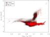 |
Fig. 1 Temperature vs. gravity of all Kepler Q3 stars (black) using KIC parameters. The active sample (Rvar ≥ 0.003) is shown in red. The blue star marks the Sun which is shown for comparison. The dashed line marks log g = 3.5 which was set to exclude giants in the following. |
3. Sample selection
In Fig. 1 we plot effective temperature vs. gravity of the whole Kepler Q3 sample (black dots) with the active stars shown in red. The selection of active stars is done automatically, i.e. without visual inspection of the light curves since the Kepler sample is huge. The active stars are selected using the so-called variability range Rvar (Basri et al. 2010, 2011). The value is computed as follows: we sort the 4 h boxcar smoothed differential light curve by amplitude, cut the upper and lower 5%, and take the difference between top and bottom amplitude. This measure accounts for the intrinsic variability of the star, i.e., a variable star has a larger variability range than a quiet star. After visual inspection of several light curves we found that a suitable criterion is Rvar ≥ 0.003 (3 parts per thousand). Most of the active stars populate the dwarf regime with log g ≳ 4. The upper-right corner shows a significant fraction of active cool stars with log g ≲ 3. Visual inspection of these low gravity stars reveals two groups of variability. The first one has very high ranges up to several percent, regular spot-like variations, and long periods. This might indicate spots or pulsations on giants, which we do not consider in this work. The second group exhibits irregular variability on short time scales that could be due to multiple mode pulsations. The Sun (blue star) is shown for comparison. All parameters have been taken from the Kepler Input Catalog (KIC). We see that the Kepler sample is strongly biased towards solar-like stars, but also a large giant branch (log g ≲ 3.5) is clearly visible.
We compared this value to total solar irradiance (TSI) data from the VIRGO instrument at the SOHO satellite. Using data from Dec. 01 1995−Sep. 01 2011 we found that the maximum range was max(Rvar, ⊙) = 0.0023, with a mean of ⟨Rvar, ⊙⟩ = 0.0011 during solar maximum (Feb. 20 1999−Oct. 21 2004). This value lies below our limit, thus all stars considered are more active than the active Sun. The variability range is our key measure to distinguish between active and quiet stars, i.e., all stars with Rvar above the upper limit will be called active although there is a large spread in their ranges; 40 661 stars of the whole Kepler sample survive this criterion. The distribution of ranges is shown in Fig. 2. Only 24.6% of all stars are considered active, i.e., to these stars we will apply the analysis procedure from Paper I.
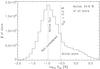 |
Fig. 2 Distribution of Rvar for all Kepler Q3 stars. 40 661 active stars lie above the imposed limit Rvar ≥ 0.3% that excludes more than 75% of all stars. |
4. Period determination
Stellar activity covers a wide field of different phenomena. Our main focus is the detection of periodic variability induced by dark spots co-rotating with the star. Since the spot periods constrain the stellar rotation law the detection of more than one dominant period is considered a hint for DR although there might be other effects able to mimic DR. Hence, the method from Paper I is applied to all active stars defined in the previous section. In Sect. 4.1 we briefly recall our method for detecting different periods in a light curve (for details we refer the reader to Paper I), and describe the selection process for achieving the physically meaningful periods (Sect. 4.2). In Sects. 4.3 and 4.4 we apply different filters to the set of returned periods to make sure that rotation is their favorite explanation. Finally, we show three examples where DR is the favorite explanation for the light curve pattern (Sect. 4.5).
4.1. Lomb-Scargle periodogram and pre-whitening
To detect periods in a light curve we used the generalized Lomb-Scargle periodogram (Zechmeister & Kürster 2009). To save computation time each light curve was binned to two hour bins. The lowest frequency is given by the inverse product of the time span (≈90 days) times an oversampling factor of 20, i.e., flow ≈ 1/(90 × 20 d), which accounts for proper frequency sampling. Using a denser frequency sampling (factor of 30) did not change the results. The highest frequency is given by the Nyquist frequency using the above binning. The binning does not affect the period determination since we only considered periods longer than half a day (Sect. 4.2).
Computing the Lomb-Scargle periodogram is equivalent to fitting a sine wave to the data. Subtracting the sine function from the data and computing the periodogram of the residuals yields a second period. This pre-whitening procedure was repeated five times to detect additional periods in the light curve. Afterwards, all sine parameters were used as input for a global sine fit which is a simultaneous fit of the sum of all five sine waves allowing for all periods to vary. Using more pre-whitening steps results in a better fit, but is computationally intensive and does not yield new significantly different periods. The enlarged set of returned periods makes it more difficult to assign a physical meaning to the individual periods (Sect. 4.2). Visual inspection of several light curves confirmed that the resulting fit was sufficient to detect significant rotation-induced periods. Three example light curves, the resulting fits, and the corresponding periodograms are discussed in Sect. 4.5.
4.2. Period selection
The next step was to select the most significant periods from the global sine fit, and to assign a physical meaning to them. We were interested in rotation periods of the star. The whole concept of only one rotation period is not quite exact, because one can only detect periodic variations caused by active regions located at certain latitudes. We think of either single spots or spot groups rotating over the visible hemisphere. If these regions are not located at the equator, then the equatorial rotation period remains unknown. Another problem arises from stars with a high spot coverage due to many small spots. If their surface distribution is inhomogeneous, then their light curves cannot be distinguished from a star with few active regions. Nevertheless, we used the first sine period from the global sine fit as the most significant period in the light curve. This period belongs to the highest power found in the pre-whitening process, and is therefore defined as one rotation period. In some cases the spots are located on opposite sides of the star, and the half period is what was detected. To minimize these alias periods we compared the first two periods from the global sine fit. If the difference of twice the first period and the second period is less than 5%, then the algorithm selected the longer one, which is more likely the correct period. The period finally selected is our primary period P1.
If the star rotates differentially, active regions have different velocities that manifest in a superposition of different periods in the light curve. To search for a second period close to P1, we looked for a period P2 within 30% of P1 in the remaining four sine periods. To estimate the relative surface shear of the two active regions we defined  (3)with Pmax = max { P1,P2 }. Since we cannot tell from the light curve whether the star rotates solar-like or anti-solar-like, we always assumed solar-like DR. To get closest to the total equator-to-pole shear we normalized the period difference by Pmax. Equivalent to Pmax we defined Pmin = min { P1,P2 } to get closest to the equatorial period. The value of α should hold the relations
  (4)The upper limit αmax = 0.3 was a reasonable choice because the solar value is α⊙ = 0.2, and the total amount of DR is unknown for stars other than the Sun. In Appendix A we showed that the general results were not affected by using different αmax values. The lower limit αmin = 0.01 accounts for the fixed frequency resolution of the periodograms. If there were more than one sine period satisfying both criteria, then the one with the second highest power in the pre-whitening process was chosen. If P1 was an alias period, then only the remaining three sine periods were considered to look for a second period.
In contrast to previous studies we found that the highest peak of the initial periodogram was a bad measure for filtering out active stars. The periodogram often detected a period longer than 90 days. These long periods remain doubtful because one cannot distinguish between remnants from the PDC-MAP pipeline and real long-term variability. Their peak height in the periodogram was similar to more reliable shorter periods, i.e., the peak height was highly biased by the data reduction. Thus, the variability range was the only measure we used.
Now, we make further restrictions to the derived periods to assure that these are really due to rotation. Using the variability range, we selected 40 661 active stars from the whole sample. As seen in Fig. 1 there were several active giants. Since we are mainly interested in rotation periods of main-sequence stars, the surface gravity was restricted to log g > 3.5 marked by the black dashed line in Fig. 1. Further limits were applied to the period P1 setting 0.5 d ≤ P1 ≤ 45 d. The lower limit should exclude pulsations, which mostly occur on timescales shorter than half a day. The upper limit is approximately equal to half the time span of Q3. Since Kepler suffers from instrumental effects visible on timescales of the quarter duration, periods longer than 45 days remain doubtful. We cannot distinguish between long-term variability, and trends caused by the instrument, because the periods were selected automatically by our algorithm. Nonetheless, there exists a certain fraction of stars with long periods. We cannot be sure that some of them are also due to instrumental effects, so they should be treated with some caution. Furthermore, all derived periods P1 for relevant stars are compared to the orbital periods Porb from the lists of eclipsing binaries3 and false positives4. If the relation | P1 − Porb | /Porb < 0.05 holds, these periods were discarded. This limit excludes orbital periods, but we might lose some tidally locked systems.
4.3. Zero crossings
After setting several constraints to P1, we applied a filter to achieve periods originating from rotating active regions by counting the number of zero crossings of each light curve. For many possible realizations of a spotted star, the light curve showed a sine-like variation with a defined number of zero crossings. Thus, a low number of crossing events was indicative for regular rotation-induced variations, whereas a high number of zero crossings was considered a hint for stellar pulsations and irregular variations. In this way we filtered out periods that did not originate from rotation.
A single sine wave has two zero crossings per period. Thus, the number of zero crossings in Q3 equals Nzero = 90 × 2/P1 = 180f1 for a sine wave with a period P1. To calculate Nzero the light curves had to be smoothed. Since we were facing a variety of different rotation time scales (0.5−45 days), we could not apply the same smoothing width to all light curves. The very fast rotators can only be smoothed on a few hours to stay below the rotation period. For the very slow rotators other effects (e.g. granulation) becomes dominant on these time scales so the smoothing time needs to be sufficiently longer. To account for this effect, we smoothed the light curves over timescales proportional to their period P1. Since Kepler long cadence data consists of ≈30 min integrations, we had 48·P1 data points in a certain period P1. We smoothed the data using a boxcar average with a width of 4 × P1 data points, which turned out to be a suitable width for fast and slow rotators. We plot the frequency f1 vs. the number of zero crossings in Q3 in Fig. 3.
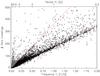 |
Fig. 3 Frequency f1 vs. number of zero crossings in Q3. The lower red line equals the number of zero crossings expected for sine-like variations. Stars lying above the upper red line (gray symbols) were discarded because they show more than twice the number of zero crossings expected. |
The lower red line equals Nzero = 180 × f1 as predicted for sine-like variations. The upper line equals 2Nzero = 90 × 4/P1. This upper limit accounts for the cases of two active longitudes located on opposite sides of the star, which produces up to four zero crossings per period. This trend was broken toward longer periods; the variations became irregular showing more zero crossings. A simple explanation is that the smoothing width chosen was too small. Another reason could be that star spots evolve on these long time scales (P1 > 20 days) as seen on the Sun. Stars with too many zero crossings were considered irregular, quiet, pulsators, or giants with poorly determined log g. All stars lying above the upper red line (gray symbols) were discarded.
4.4. Detection limit of α
After filtering out periods by their number of crossing events, we focused on the cases where two periods were found. The reliability of a second period strongly depends on the separation of the periods P1 and P2 in the periodogram. If they lie very close it is hard to tell whether the small separation comes from a very small α, or if it is due to artifacts from our method. After visual inspection of several light curves we found that the typical separation of the two periods should be larger than ten points on the frequency grid in the periodogram. Thus, we inverted the periods to achieve two frequencies f1 = 1/P1 and f2 = 1/P2. If their absolute separation was less than ten times the lowest frequency flow (Sect. 4.1), i.e., | f1 − f2 | < 10flow ≈ 0.0056 cycles d-1, then the second period was discarded.
For each of the above limits imposed upon the set of periods, we might have lost real rotation periods. This was not preventable, because the analysis procedure was done automatically. All filters applied have decreased the number of false-positives significantly, yielding a condensed and reliable set of rotation periods. We found that 24 124 stars survived all filters, i.e., they have a measured rotation period P1. For 18 616 stars a second period P2 was found. The following section shows example light curves, the fits achieved by our method, and the associated periodograms. It demonstrates the problem of determining a second period from the periodograms, and shows the importance of pre-whitening.
4.5. Examples: light curves, periodograms, and rotation periods
We briefly address the problem of associating the returned periods from the pre-whitening to rotation periods of active regions on the star. Figure 4 shows an example of a fast rotator, KIC 1995351, and the associated periodograms. The upper panel shows the light curve and the global sine fit of all five periods in red. The light curve shows a regular beating pattern most probably due to several active regions. The lower panel shows (from top to bottom) the first to the fifth periodogram. The highest peak in each periodogram was marked by a vertical red line.
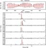 |
Fig. 4 Top Panel: light curve and global fit of the star KIC 1995351. Lower Panel (top to bottom): periodograms 1–5. The vertical red lines indicate the highest peak in each periodogram. The periods P1 = 3.24 d and P2 = 3.57 d were selected by our method. |
The first periodogram reveals several distinct peaks close to the most significant one at 3.24 days, which was chosen as primary period P1. In the second panel the periodogram of the residuals was taken. One clearly sees that the power of the peak around P1 = 3.24 days dropped to zero, whereas the second and third highest peak from the initial periodogram now exhibit the highest powers. The period with the second highest power around P2 = 3.57 days was chosen. From the third to the fifth panel we see that there are more periods close to P1 probably due to other active regions. In the fourth periodogram the vertical red line is not visible because the highest peak lies at 63.6 days, which is most probably an artifact from the data reduction. The periodogram fits long-term trends in the light curve with periods much longer the rotation periods.
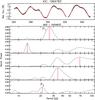 |
Fig. 5 Top Panel: light curve and global fit of the star KIC 1869783. Lower Panel (top to bottom): periodograms 1–5. The vertical red lines indicate the highest peak in each periodogram. The periods P1 = 26.2 d and P2 = 20.9 d were selected by our method. |
In Fig. 5 we show the slow rotator KIC 1869783 and the associated periodograms. The panels are the same as in the previous plot. The light curve has a double-dip shape due to active regions located on opposite sides of the star. The initial periodogram shows a rather broad peak at 26.2 days that was chosen as primary period P1. The second periodogram shows a peak around 13.1 days that belongs to the second active region on the opposite side of the star. From the light curve we can see how this region becomes shallower, and the primary region more pronounced. This traveling wave is usually interpreted as migrating star spots. The third periodogram has the highest peak around 68.5 days. Again, this peak most probably results from the data reduction. The fourth periodogram shows a strong peak around 34.2 days that was unfortunately discarded by the selection process because it lies beyond 30% of P1. Only in the fifth pre-whitening step another period at 20.9 days was found which was chosen as P2 because it lies within 30% of P1.
These two examples demonstrate the process used to detect the most significant periods. The beating pattern seen in the light curve in Fig. 4 is no proof of DR, but that was the most probable explanation. The slow rotator shows active regions at different longitudes evolving with time. In this case it is not clear whether this was due to DR, or spot growth or decay. Both figures demonstrate that the fits to the light curves reproduce the main activity pattern. They could be improved by using more than five sine waves, but this would not change the two most significant periods. Furthermore, they point out the presence of a second period, and the difficultyof assigning a physical meaning to them.
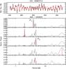 |
Fig. 6 Top Panel: light curve and global fit of the star KIC 9580312. Lower Panel (top to bottom): periodograms 1–5. The vertical red lines indicate the highest peak in each periodogram. The periods P1 = 3.97 d and P2 = 4.86 d were selected by our method. |
Finally, we discuss the example of an F-type star in Fig. 6. This particular star has an effective temperature of Teff = 6504 K and a color index of B − V = 0.47 (see Sect. 5.2), which roughly corresponds to a spectral type of F6V. It is questionable whether the variability in the light curve results from star spots because F stars are known to exhibit very thin convection zones. Our pre-whitening analysis reveals the two most significant periods P1 = 3.97 d and P2 = 4.86 d. The second periodogram shows an alias of P1 around 2 days. The highest peak in the fourth periodogram yields a period of 37.1 days that corresponds to the beating pattern. The fifth period found is located at 4.52 days which lies between P1 and P2. Figure 6 clearly shows that the fit to the light curve is worse than in the other two examples, but still sufficient to reveal the two strongest periods. In this case, the beating pattern most probably results from differentially rotating spots, although this light curve shape was also observed in γ Dor stars. We discuss this issue in more detail in Sect. 5.5.
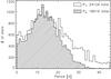 |
Fig. 7 Distribution of rotation periods for the 24 124 stars with period P1 and the 18 616 stars with second period P2 with weighted means of 16.3 and 13.3 days, respectively. The distribution of P2 falls off more rapidly towards 30 days because instrumental effects currently hamper the detection of long periods. |
5. Results
In this section we present rotation periods of more than 20 000 Kepler stars. Section 5.1 compares our results to previous measurements and Sect. 5.2 shows that our periods are consistent with the concept of magnetic braking. Our main focus is on the detection of DR, which is discussed in terms of relative and absolute shear in Sects. 5.3 and 5.4, respectively. Finally, we estimate the number of false-positives, i.e., those periods mis-classified as rotation in Sect. 5.5, especially accounting for stars hotter than 6000 K.
5.1. Rotation periods
In Fig. 7 we show the distribution of the rotation periods P1 and P2. We found ⟨P1⟩ = 16.3 d and ⟨P2⟩ = 13.3 d, with a spread of σ(P1) = 10.1 d and σ(P2) = 7.3 d, respectively. The distribution of P1 slightly decreases toward longer periods, and levels off around ≈35 days. Toward shorter periods a second peak between 0.5 and 2 days appears. The distribution of P2 falls off more rapidly towards long periods. Most of the missing periods P2 are greater than 20 days, so some of them might lie below our detection limit. Thus, the mean values of the distributions do not necessarily indicate that a second period is more likely be found for shorter periods. There are several explanations for the dearth of slow rotators in both distributions. The determination of long periods requires stable active regions on the star. On the Sun the spot lifetimes are of the order of the rotation period hampering the period detection. This does not need to be true for other stars, however. Furthermore, long-term stellar variability and instrumental trends are currently difficult to distinguish in Kepler data. Both effects bias the distribution towards shorter periods. Our results apply primarily to periods shorter than about 30 days. Since we have analyzed only one quarter so far, and applied an upper limit of 45 days, the distribution of slow rotators is not addressed in this study.
5.2. Rotational braking
It is well-known that stellar rotation rates correlate with spectral type. Stars around spectral type F and earlier are known to be fast rotators. The convection zone grows towards cooler stars, and a dynamo mechanism generates magnetic fields. Ionized material follows the magnetic field lines (stellar wind) and carries away angular momentum resulting in a spin-down of the star (Barnes 2003; Reiners & Mohanty 2012). This process is known as rotational braking, for which we show evidence in Fig. 8. We plotted our most significant period P1 against B − V for 24 124 stars with at least one detected period (gray dots). Figure 8 is a composition of previous rotation studies and our results. Filled circles represent data from Baliunas et al. (1996), Kiraga & Stepien (2007), Irwin et al. (2011), and recently McQuillan et al. (2013) published rotation periods for the Kepler M dwarfs sub-sample. For some of those measurements no B − V information was available. We transformed stellar masses into effective temperature using 1 Gyr isochrone models from Baraffe et al. (1998). The temperatures have been transformed into B − V using the relation from Reed (1998). For the Kepler stars we used the relation between g − r and B − V from Jester et al. (2005). The periods from Baliunas et al. (1996) form an upper envelope to our results. The results for the Kepler M dwarfs (blue circles) show good agreement with our results (see also Fig. 16), although McQuillan et al. (2013) used an auto-correlation method which is a completely different mathematical tool.
Figure 8 is consistent with the picture of rotational braking. A steep rise in rotation periods appears around B − V ≈ 0.6. In this region the convection zone starts to form, and grows deeper in cooler stars. Thus, magnetic braking becomes stronger leading to a spin-down of the stellar rotation rate. Barnes (2007) empirically found a relation between B − V, age t, and rotation period:  (5)The age-dependence is similar to the classical Skumanich law
  (see also Reiners & Mohanty 2012). The black curves in Fig. 8 represent isochrones with ages of 100, 600, 2000, and 4500 Myr. The distribution of periods in our sample follows a similar behavior as the isochrones indicating that stars with different color follow similar age distributions. Stars with rotation periods around 5 days are probably very young stars that did not have time to spin-down. In Fig. 9 we show rotation period P1 vs. range Rvar in a density plot. The bright region in the middle represents a high density, whereas dark regions express low density. Young stars are expected to be fast rotators but also to be very active. We found that the range increases toward fast rotation, supporting this relation between our measured rotation period and variability range. Hence, the variability range is a useful age and activity indicator.
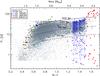 |
Fig. 8 B − V color vs. rotation period P1 of the 24 124 stars with at least one detected period (gray dots). The filled circles represent data from Baliunas et al. (1996, olive), Kiraga & Stepien (2007, purple), Irwin et al. (2011, red), and McQuillan et al. (2013, blue). Towards cooler stars we found an increase in rotation periods with a steep rise around B − V ≈ 0.6 supplying evidence of rotational braking. The black lines represent a color-period relation found by Barnes (2007) for different isochrones. The four stars mark the position of the Sun (blue), KIC 1995351 (cyan), KIC 1869783 (purple), and KIC 9580312 (red) for comparison. |
We estimated the ages from the rotational period for the Kepler stars using Eq. (5). The distribution of ages in the active Kepler stars is shown in Fig. 10. The black histogram shows all stars with 0.5 < B − V < 1.0, the red one covers 1.0 < B − V < 1.4, and the blue one shows 1.4 < B − V < 1.5. The steep decrease on the right-hand side of all three distributions can be understood by the missing long-period stars caused by our upper limit of 45 days, and by our selection of active stars only. The left-hand side of the age-distribution is expected to be almost complete because the lower limit of detectable periods of 0.5 days is not relevant even for very young active stars. The dashed black line shows the distribution of stars according to a uniform distribution of stellar ages (plotted on a logarithmic scale). The dashed curve is remarkably similar to the left-hand side of the black distribution up to an age of ≈300 Myr.
McQuillan et al. (2013) found evidence for a bimodal period distribution in the Kepler M dwarf sample (1.21 < B − V < 1.62). The bimodality is explained by the existence of two distinct stellar populations. The gap at P1 ≈ 30 days also appears in our data around 1.4 < B − V < 1.5, corresponding to an age of roughly 800–900 Myr. We found a similar feature in hotter stars (1.0 < B − V < 1.4) at P1 ≈ 20 d. This feature, however, corresponds to a significantly younger age of 600–800 Myr, and is unlikely to be caused by the same age distribution as the gap in cooler stars. Whether the two period gaps are caused by a selection bias affecting our period sample, or by a predominance of certain ages in the distribution of stellar ages (potentially introduced by stellar clusters in the Kepler field; see, e.g., Meibom et al. 2011) needs to be tested. Furthermore, in comparison to a constant star formation history (dashed red line in Fig. 10), the sample with 1.0 < B − V < 1.4 (red histogram) lacks stars younger than ≈200 Myr. The dearth of young objects and the gaps in the age distributions cannot be easily explained and need further investigation. We leave this discussion for a subsequent paper.
5.3. Relative differential rotation α
In Fig. 11 we plot the relative DR α against the minimum rotation period Pmin.
We found that α increases with rotation period. The black dashed line marks the detection limit (Sect. 4.4) of our method. If we sort both periods so that P1 = Pmin and P2 = Pmax, then the absence of data points below this line can be understood by considering the relation
 Thus, all data points lie above the black line, which is the lower limit for α. It is worth noting that more than 75% of all stars with detected period P1 lie above the detection limit, because 18 616 of 24 124 stars exhibit a second period. In other words, only the 5505 stars where only one period was detected can either lie below the detection limit, or above (below) our αmax(αmin) values, respectively. In the Appendix we discuss different αmax values, and show that periods are found for αmax > 0.3 (see Fig. A.2), which were discarded in some cases (see Fig. 5). Lowering the value of αmin yielded essentially the same periods, so we conclude that the general trend of increasing α with rotation period was not biased by our detection limit.
The colors in Fig. 11 represent different temperature bins. Towards cooler stars (Teff < 5000 K, red and purple dots) the rotation period increases, confirming the result from Fig. 8. Hot stars above 6000 K (green and black dots) mostly populate the short periods covering the whole α range. This region is probably biased by pulsators, which was considered in Sect. 5.5.
In Fig. 12 we show temperature vs. α, correlating our results with the variability range. The colors indicate different ranges growing from 0.3% (yellow) to high ranges with amplitudes above 5% (purple). A shallow trend towards higher α with decreasing temperature is visible (see also Fig. A.1). A correlation with range can only be found for stars with very high ranges (purple dots). These stars mostly cover the region with α ≲ 0.05 over a large temperature range. If we think of the variability range as an activity indicator this might confirm the hypothesis that these stars are very young, because low DR α indicates short periods.
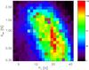 |
Fig. 9 Density plot of rotation periods P1 vs. Rvar with bright regions representing a high density, whereas dark regions express low density. The annotation of the color bar contains the total number of stars in each bin. The distribution shows that the range increases towards shorter periods. Since fast rotators are expected to exhibit an enhanced level of activity, the range could probably be used as proxy for stellar activity. |
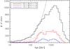 |
Fig. 10 Distribution of ages inferred from rotation periods P1 for different color bins. For B − V > 1.0 (red and blue) we found a bimodal distribution in agreement with McQuillan et al. (2013). The dashed black and red lines show uniform age distributions (on a logarithmic scale). |
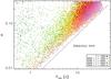 |
Fig. 11 Rotation period Pmin vs. α for all stars with two detected periods. The colors represent different temperature bins, the dashed black line marks the detection limit. The relative shear α grows towards longer rotation periods. More than 75% of all stars with detected period P1 exhibit a second period P2, and lie above the detection limit. This trend cannot be broken by the 5505 stars with only one detected period, because most of the missing stars lie above the upper limit αmax = 0.3. |
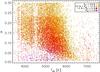 |
Fig. 12 Effective temperature vs. relative shear α. We found that α slightly increases towards cooler stars. The colors indicate different variability ranges. A distinct correlation between α and the range is only visible for the stars with very high ranges Rvar > 5%. These stars group at small α values over a large temperature range. Low α represents short periods, probably indicating that their young age. |
5.4. Absolute horizontal shear ΔΩ
We define the absolute horizontal shear as
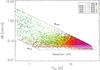 |
Fig. 13 Rotation period Pmin vs. absolute shear ΔΩ. The colors are the same as in Fig. 11, the detection limit is marked by the horizontal dashed line, and the diagonal dashed lines mark the upper and lower limit αmax and αmin, respectively. We found that ΔΩ is independent of Pmin over a large period range, although the upper and lower limit suggest an increase of ΔΩ towards short periods, showing large scatter on one order of magnitude. |
In Fig. 13 we plot ΔΩ against the rotation period Pmin. The colors are the same as in Fig. 11; the detection limit is marked by the horizontal dashed line; and the diagonal dashed lines mark the upper and lower limit αmax and αmin, respectively. For periods longer than two days, ΔΩ shows weak dependence on rotation period. Below two days, ΔΩ shows large scatter on the order of one magnitude. The upper and lower limits suggest that ΔΩ increases toward short periods, which is not necessarily the case (see Fig. 14).
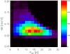 |
Fig. 14 Density plot in the Pmin − ΔΩ plane. For ΔΩ < 0.10 rad d-1 the total shear does not depend on rotation period. For ΔΩ > 0.10 rad d-1 we found large scatter of ΔΩ from fast to moderate rotators. |
Previous observations (Barnes et al. 2005) and theoretical approaches (Küker & Rüdiger 2011) also showed weak dependence of ΔΩ on rotation period. To emphasize this result in our measurements, we show a density plot in the Pmin − ΔΩ plane in Fig. 14. In the range 0.035 rad d-1 ≲ ΔΩ ≲ 0.10 rad d-1 the absolute shear does not depend on rotation period. Above 0.10 rad d-1 the shear shows large scatter for periods 0.5 d ≲ Pmin ≲ 15 d. Again, the upper limit αmax (see Fig. 13) suggests a trend toward fast rotators.
Figure 14 is similar to Fig. 3 in Küker & Rüdiger (2011) showing the dependence of ΔΩ on rotation period for different stellar mass models. These authors found weak dependence of ΔΩ on rotation period for all masses. Their model curves would fit our observations in Fig. 14, although the 0.5 M⊙ and 0.3 M⊙ models lie below our detection limit. Küker & Rüdiger (2011) did not consider high DR ΔΩ > 0.1 rad d-1, but their 1.1 M⊙ model exhibits the largest value of ΔΩ, and deviates the most from the almost constant shape of the other models, which could be a hint for the different behavior in this regime.
The temperature dependence of ΔΩ is shown in Fig. 15. Our results reveal two distinct temperature regions showing different behavior of ΔΩ. For temperatures ranging from 3500−6000 K, ΔΩ shows only weak dependence on temperature. Above 6000 K, ΔΩ steeply increases toward hotter stars, but with large scatter supporting no conclusion about the functional form of a fit. Barnes et al. (2005) found a strong temperature dependence of ΔΩ supplying the power-law  . This was confirmed by Collier Cameron (2007) supplying the power-law fit ΔΩ = 0.053 (Teff/5130)8.6.
Our results show good agreement with theoretical curves provided by Küker & Rüdiger (2011). These authors found that the temperature dependence of ΔΩ cannot be represented by a single power-law fit, but requires two fits for different temperature regions (red and light blue curve; compare Fig. 2 in Küker & Rüdiger 2011), which was clearly confirmed by our measurements. For temperatures of 3500−6000 K, Küker & Rüdiger (2011) predict a shallow increase of ΔΩ (red dash-dotted line). Since this behavior is not evident in Fig. 15, we calculated histograms of ΔΩ for temperature bins of 250 K between 3400 K and 7400 K. For each distribution, i.e., for each temperature bin, the weighted mean ⟨ΔΩ⟩ was calculated, and is shown as an open black circle in Fig. 15. The mean values slightly increase for temperatures of 3500–6000 K. Above 6000 K ⟨ΔΩ⟩ shows very good agreement with the light blue dashed curve, as predicted by Küker & Rüdiger (2011). For even hotter stars (Teff > 7000 K) the derived periods are most probably highly contaminated by pulsators (see Sect. 5.5). In this region the derived periods and ΔΩ values should be treated with caution, which is indicated by the vertical red bar.
Although our measurements suggest good agreement between theory and observations in both regions, the results should be treated with caution. For the 5505 stars, for which only one period was detected, we cannot tell whether these stars exhibit a small horizontal shear below our detection limit, or if a second period was not detected for other reasons. A fraction of these 5505 stars can change the trends we found, so we cannot draw strong conclusions about the behavior below the lower limit ΔΩ ≈ 0.035 rad d-1.
5.5. False positives
In this section we statistically estimate the number of periods in our final sample that survived all filters but are probably not due to rotation. Other sources of periodic stellar variability are binarity, pulsations, or instrumental effects, for example. We call these detections false positives (FPs). We defined three classes of rotational variability: the rapid rotators (0.5 d < P1 < 10 d), the moderate rotators (10 d < P1 < 20 d), and the slow rotators (P1 > 20 d). Example light curves representative of the first and last group are shown in Figs. 4 and 5. Figure 6 shows an example of an F star. These hot stars are investigated separately at the end of this section. Since the sample is too large to inspect each light curve individually, we randomly selected 100 stars of each rotation class and checked their light curves by eye. This will only give a rough error estimate, because only a small number of stars was inspected, and the method remains very subjective.
Orbital periods of eclipsing binaries or transiting planets should be relatively rare in the final sample. The eclipsing binary list3 was cross-matched with our sample, and stars with coinciding KIC numbers were discarded. For stars hosting planets or planetary candidates, the returned periods were predominantly due to stellar activity. The transits cover very few data points compared to rotational modulations, hence the periodogram is not very sensitive to these periods. We found no period associated to eclipsing binaries or planetary transits in this test.
 |
Fig. 15 Effective temperature vs. horizontal shear ΔΩ summarizing different measurements: the olive diamonds and error bars were taken from Barnes et al. (2005), the olive dashed curve from Collier Cameron (2007). Orange diamonds and error bars show measurements from Ammler-von Eiff & Reiners (2012). Our measurements are shown as gray dots. The red dash-dotted line and the light blue dashed line show theoretical predictions from Küker & Rüdiger (2011). The black dashed line marks our detection limit. The four stars mark the positions of the Sun (blue), KIC 1995351 (cyan), KIC 1869783 (purple), and KIC 9580312 (red) for comparison. The vertical red bar indicates stars hotter than 7000 K with probable large contamination of pulsators. The open black circles represent weighted means of our measurements for different temperature bins. From 3500−6000 K, ΔΩ shows only weak dependence on temperature. Above 6000 K the shear strongly increases as reported by Barnes et al. (2005) and Collier Cameron (2007). The different behavior of ΔΩ in these two temperature regions was supported by theoretical predictions from Küker & Rüdiger (2011, red and light blue lines). |
The rapid rotators class exhibits six stars showing irregular variations, which could be a hint for stellar pulsations (see below), six alias periods, and two periods without any reference to the light curve.
For the moderate rotators class, alias periods were the biggest error source. In six cases the detected period was most probably half of the true rotation period, and in one case the determined period could not be confirmed by visual inspection of the light curve.
The slow rotator class with periods greater than 20 days mostly suffers from instrumental effects. After each third of a quarter (≈30 days), data is down-linked to Earth cutting the quarter into three segments. Each raw data segment shows individual trends, which were corrected by the PDC-MAP pipeline. Thus, on time scales longer than 30 days, the accuracy of the derived periods strongly depends on the data reduction pipeline. Furthermore, we expect that star spots like those seen on the Sun may evolve for stars with solar rotation periods. Spot evolution distorts the light curve shape and makes it more difficult to detect stable periods. In this class only one alias period was detected, but 12 stars that did not show clear counterparts to the rotation period in the light curve (like regular dips or double dips as seen for fast rotating stars).
In total 300 stars were inspected. Summarizing results for the above rotation classes, we found that about 12% of all derived periods should probably be attributed to sources of periodic variability other than rotation.
As is evident from Fig. 11, stars hotter than 6000 K mostly exhibit periods less than 1–2 days. This regime is highly biased by pulsations (Debosscher et al. 2011), because F-type and hotter stars exhibit very thin convection zones. Fast pulsators like δ Scuti stars show pulsations on timescales of less than half a day. Thus, we set a lower limit of 0.5 days to our periods in Sect. 4.2. But there do exist hot A-type stars with γ Doradus pulsations with periods of 0.5–4 d (Balona 2011, 2013; Balona et al. 2011). Moreover, these stars show beat-shaped light curves similar to spot-induced variability. To check whether the periods found are due to rotation or pulsation, we defined three groups of hot stars following the classification of Table 1 in Balona (2011): F9-F5 stars with 6000 K < Teff < 6500 K, F5-F1 stars with 6500 K < Teff < 7000 K, and hotter stars with Teff > 7000 K. Again, for each group we randomly selected 100 stars, and checked their variability by eye. If a traveling wave was found in the light curve, which was visible over several periods, we interpreted this behavior as migrating spots (see Fig. 6) indicating DR.
For the F9-F5 stars: the derived periods are mostly rotation-induced. Only six stars were misclassified: two probable pulsating stars, three stars showing irregular variability, and one eclipsing binary. In the second group (F5-F1 stars), beat-shaped light curves are found quite frequently. In thirty-three stars no traveling wave was found, although some of them exhibit a beat-shaped light curve. Thus, the variability probably arises from pulsations.
The situation becomes even worse for the hottest stars. Thirty-seven stars without moving dips were found, five periods without clear reference in the light curve, and three alias periods. This group shows the biggest contamination by γ Dor or extreme δ Scuti pulsators. Although it is challenging to distinguish between rotation and pulsation from the light curve alone, short periods of hot stars should be treated with caution.
6. Discussion
6.1. Comparison to other observations
The rotation periods of the active Kepler stars are consistent with previous rotation measurements (Fig. 8), supporting the picture of stars losing angular momentum as a result of stellar winds that has been deduced from a long history of observations.
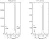 |
Fig. 16 Comparison of periods from Nielsen et al. (2013, left panel) and McQuillan et al. (2013, right panel) with the periods P1 from Fig. 8. We found good agreement with both samples, although the auto-correlation method from McQuillan et al. (2013) was less prone to alias periods than our method, as is obvious from the missing peak around 0.5 in the right panel. |
Recently, Nielsen et al. (2013) and McQuillan et al. (2013) presented rotation periods for a large sample of Kepler stars. To create confidence in our results and the method we used, we compared our periods P1 to the periods derived by these authors. The left panel in Fig. 8 shows the normalized period difference (P1 − PNielsen)/P1. In total 9292 periods were compared. The huge peak around zero shows that our periods are consistent with the periods derived in Nielsen et al. (2013), which were derived from analyzing multiple Kepler quarters. The small peak at − 1 indicates the cases where we detected an alias period P1 = PNielsen/2. The small peak around 0.5 shows the opposite effect when Nielsen et al. (2013) detected an alias according to PNielsen = P1/2. Both peaks are of the same size as expected, because the Lomb-Scargle periodogram was used in both studies.
The right panel in Fig. 8 shows the normalized period difference (P1 − PMcQuillan)/P1 comparing 1277 periods in total. Again, we found good agreement between both samples. The peak at − 1 indicating the cases where we detected an alias period P1 = PMcQuillan/2 is rather large compared to the peak around zero. This was also expected since M-dwarfs exhibit long rotation periods bearing the risk of aliasing, especially when using an automated method. Around 0.5 there is no peak visible, clearly demonstrating that the auto-correlation method used in McQuillan et al. (2013) was less prone to alias periods than our method.
Our results on DR are quite different than what was observed before. In contrast to previous observations, e.g., (Barnes et al. 2005; Collier Cameron 2007), we found that ΔΩ weakly depends on temperature for the cool stars (3000–6000 K). Above 6000 K, ΔΩ increases with temperature and the stars show no systematic trend, but seem to be randomly distributed in this temperature regime. Using Doppler imaging (DI) Barnes et al. (2005) found that the horizontal shear ΔΩ strongly depends on effective temperature  . Five stars of their sample lie below our detection limit (see Fig. 15). Collier Cameron (2007) combined results from DI and the Fourier transform method yielding the equation ΔΩ = 0.053 (Teff/5130)8.6. The two groups we found (above and below 6000 K) were also consistent with recent theoretical studies (see Sect. 6.2).
The relation between rotation period and DR has been studied by several authors. Hall (1991) found that the relative horizontal shear α increases towards longer rotation periods. Donahue et al. (1996) confirmed this trend finding ΔP ≈ ⟨P⟩1.3 ± 0.1 independent of the stellar mass. Using the Fourier transform method Reiners & Schmitt (2003) also found that α increases with rotation period for F-G stars. This result was confirmed by Ammler-von Eiff & Reiners (2012) who compiled previous results and new measurements for A-F stars. Barnes et al. (2005) found that ΔΩ only weakly correlates with rotation rate according ΔΩ ≈ Ω0.15.
Observations of DR cover a wide range of α values. Doppler imaging is particularly sensitive to small DR limited by the spot lifetimes, α ≲ 0.01 (see, e.g., measurements by Donati & Collier Cameron 1997 for AB Dor), although there were measurements (Donati et al. 2003) yielding α ≈ 0.05 for LQ Hya, and new measurements (Marsden et al. 2011) that found values between 0.005 ≲ α ≲ 0.14. The Fourier transform method (e.g. Reiners & Schmitt 2003) is sensitive to α > 0.1 and was used to determine surface shears as large as 50% for some A-F stars. With our method we are able to detect DR up to α < 0.5. The errors for individual periods are usually small. Bad detections of α result from the spot distribution on the stellar surface, which is a general problem for DR detections from photometric data. The measured shear α will always be lower than the total equator-to-pole shear. The accuracy of our method was discussed in Reinhold & Reiners (2013).
In the following we compared our results with previous rotation measurements of individual Kepler stars (see Table 1). For three Kepler stars (KIC 8429280, KIC 7985370, KIC 7765135) DR has been measured (Frasca et al. 2011; Fröhlich et al. 2012) fitting an analytical spot model to the data. Their findings showed good agreement to our results and have been compared in Paper I.
Comparison with previous rotation measurements for individual Kepler stars.
Several Kepler stars were measured by Savanov using a light curve inversion technique that constructs a map of surface temperature. Savanov (2011b) considered the planet-candidate host stars KOI 877 and KOI 896 (KIC 7287995 and KIC 7825899, respectively) finding rotation periods of 13.4 and 25.2 days, respectively, stating that both stars exhibit active longitudes separated by about 180°. For KIC 7287995 we found P1 = 13.5 d and P2 = 10.4 d, and for KIC 7825899 P1 = 12.4 d. In the latter case the detected period was an alias of the true rotation period due to the active longitudes.
The K dwarf KIC 8429280 was studied in Savanov (2011a), who found brightness variations with periods of 1.16 and 1.21 days, consistent with the results from Frasca et al. (2011). In this case we found P1 = 1.16 d and P2 = 1.21 d.
The fully convective M dwarf GJ 1243 (KIC 9726699) was studied in Savanov & Dmitrienko (2011) yielding a rotation period of 0.593 days. Our algorithm detected a period of 118.7 days due to improper data reduction in Q3. This period was filtered out by the upper limit of 45 days. The second strongest period we found was 0.59 days, in good agreement with Savanov & Dmitrienko (2011). This period does not lie within 30% of the first one, and hence was not chosen as P2.
Savanov & Dmitrienko (2012) also studied the fully convective, low-mass M dwarf LHS 6351 (KIC 2164791). These authors detected a rotation period of 3.36 d, as well as evidence for DR in terms of ΔΩ = 0.006 − 0.014 rad d-1 from the evolution of surface temperature inhomogeneities, which lies below our detection limit. We found P1 = 3.35 d and P2 = 3.27 d yielding ΔΩ = 0.046 rad d-1. Visual inspection of the light curve in Q3 supports the larger value of ΔΩ, because a second active region appears after some periods, which was not observed in the Q1-Q2 data. Unfortunately, this star was discarded by our algorithm because it has no effective temperature or log g values from the KIC, and misses in our final list.
Bonomo & Lanza (2012) analyzed the active planet-hosting star Kepler-17 (KIC 10619192). These authors detected a rotation period of 12.01 d, and the existence of two active longitudes separated by approximately 180° from each other. Furthermore, Bonomo & Lanza (2012) found evidence for solar-like DR, but were not able to give precise estimates for the horizontal shear claiming that active regions on this star evolve on timescales similar to the rotation rate. We detected an alias period of 6.05 d due to the two active longitudes. Again, we found no second period within 30% of P1. Checking our second and third strongest period, we found 10.85 d and 12.28 d, respectively, in good agreement with rapid spot evolution.
Recently, Roettenbacher et al. (2013) found a period of 3.47 days for the Kepler target KIC 5110407, and evidence for DR using light curve inversion. We found P1 = 3.61 and P2 = 3.42 days yielding α = 0.053, which is consistent with their differential rotation coefficient k = 0.053 ± 0.014 for an inclination of i = 45° in their model.
Several open clusters in the Kepler field have been studied. Meibom et al. (2011) measured rotation periods for stars in the open cluster NGC 6811, supplying evidence for rotational braking (see Fig. 8). Additional measurements were done for the open clusters NGC 6866 (Balona et al. 2013a) and NGC 6819 (Balona et al. 2013b) showing rotational braking as well. The same author found several A-type stars showing signatures of spot-induced variability (Balona 2011, 2013), e.g., a beating pattern in the light curve, although this behavior was not expected because of their purely radiative atmospheres.
6.2. Comparison to theory
Solar DR has been studied theoretically for a long time. Kitchatinov & Rüdiger (1999) computed DR models for late-type (G2 and K5) stars. They found that the relative shear α increases with rotation period. They also showed that α increases towards cooler stars. The general trends are in agreement with our findings, although their range of α values lies above our values.
Küker & Rüdiger (2005a) computed models for an F8 star, and found weak dependence on rotation period, which was confirmed by later studies for F, G, and K stars (Küker & Rüdiger 2005b), showing that the dependence on temperature was much stronger. This result holds for different main sequence star models (Küker & Rüdiger 2007). These authors found that above a temperature of 5800 K the strong temperature dependence on ΔΩ claimed in Barnes et al. (2005) fits the model data reasonably well, whereas below 5800 K the data lie far off the fit. Recent studies (Küker & Rüdiger 2011) have shown that the temperature dependence of ΔΩ cannot be represented by one single power law over the whole temperature range from 3800–6700 K. Figure 2 in Küker & Rüdiger (2011) shows that ΔΩ only slightly increases with temperature for stars cooler than ≈5800 K consistent with our measurements (Fig. 15). For stars hotter than ≈6200 K these authors found that ΔΩ shows an even stronger dependence on temperature than predicted in Barnes et al. (2005). In the same temperature region, our measurements start to show a different behavior (see Fig. 15).
The weak dependence of ΔΩ on rotation period was confirmed by our measurements (see Fig. 14), as predicted by Küker & Rüdiger (2011) for different solar mass models, and other authors before. Hotta & Yokoyama (2011) modeled DR of rapidly rotating solar-type stars and found that DR approaches the Taylor-Proudman state, i.e., that ΔΩ/Ω decreases with angular velocity, as long as the rotation rate is above the solar value. This model agrees well with our findings in Fig. 11.
Direct numerical simulations showed that models with low Rossby numbers (i.e., fast rotating stars) generate strong dipolar magnetic fields (Schrinner et al. 2012). These fields amplify Lorentz forces able to suppress Coriolis forces, and hence can effectively suppress DR (Gastine et al. 2012). This result from theoretical models agrees well with the trend we found that α decreases towards shorter rotation periods (Fig. 11).
The dipolarity of the magnetic field strongly depends on the length scale of convection. As the depth of the convection zone decreases, the dipolarity breaks down rendering the rotation non-uniform (Schrinner et al. 2012). This effect could explain the strong increase of ΔΩ around Teff > 6000 K. Browning (2011) provided an explanation for the shallow increase of α towards cooler stars. Because M dwarfs exhibit low luminosities, and therefore low convective velocities, they strongly depend on the rotation rate even at solar rotation rates. Magnetic fields cannot quench DR effectively, so they exhibit strong solar-like DR.
7. Summary
We applied our method from Paper I to the active fraction of Kepler Q3 data to search for DR in high precision empirical data. We measured rotation periods of 24 124 Kepler stars, providing evidence for DR in 18 616 stars. Our measurements for the rotation period were in good agreement with previous results. Moreover they were consistent with the theory of magnetic braking.
Our measurements provide a comprehensive database of stellar DR. For the first time, we could explore a well-defined parameter range in a statistically significant sample. We found that the relative shear α increases towards longer periods, and slightly increases towards cooler stars. The absolute shear ΔΩ showed weak dependence on rotation period over a large period range. In contrast to other observations ΔΩ showed a shallow increase for temperatures from 3500–6000 K, and a steep increase above 6000 K. Periods above 7000 K should be treated with caution because of probable high contamination of pulsators. Both the dependence on rotation period and temperature were in good agreement with recent theoretical models. Furthermore, we cannot find any other reasonable explanation for the trends we found.
We interpreted the existence of a second period as DR. Although our method is not able to distinguish between DR and spot evolution, we were confident that most of our measurements reflect the stellar surface shear because they resemble previous measurements and recent theoretical models. This was the first time that DR was measured for such a large number of stars. For the future this analysis will be applied to more Kepler data to verify the rotation periods, DR, and to learn about spot lifetimes. Kepler is the natural source for answers to these questions.
Online material
Appendix A: Differential rotation beyond α = 0.3
In Eq. (4) an upper limit of αmax = 0.30 was used while searching for a second period. In this section we demonstrate how different upper limits αmax change the total number of detections and the overall behavior of α with temperature and rotation period. We use ten equidistant values 0.05 ≤ αmax ≤ 0.50 (see Table A.1). With increasing αmax we found a larger total number
Number of stars with second period found for different αmax values.
of periods. The case αmax = 0.5 is shown to demonstrate the limits of our method, which is evident in the next two figures. For all stars with two detected periods we plotted their density in the Teff − α plane in Fig. A.1. The colors are the same as in Fig. 9 with bright regions representing high density. For each αmax value we found that α slightly increases towards cooler stars. The case with the lowest upper limit (αmax = 0.05) looks a bit scattered, but it is not very different from the general trend. The plot in the lower-right corner (αmax = 0.5) demonstrates the limits of our method. Many stars jumped to the upper limit α = 0.5 because an alias period was chosen by the algorithm. The Teff values from the KIC are not very accurate and neither are the stellar radii. We found the same trend with respect to α however, i.e., the α value increases towards smaller radii (although this may not be an independent constraint).
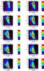 |
Fig. A.1 Density plot in the Teff − α plane for different values of αmax. For each αmax value we found that α slightly increases towards cooler stars. The plot in the lower-right corner (αmax = 0.5) demonstrates that our method is limited to αmax < 0.5. Colors are the same as in Fig. 9. |
Our previous result that α increases towards longer rotation periods holds for all αmax values. In Fig. A.2 we showed the density in the Pmin − α plane. We see that the density is localized in a sharp strip that smears out for limits greater than αmax = 0.3. These large α values belong to periods P2 longer than 45 days where instrumental effects play a dominant role. Again, the stars jumped to the upper limit in the αmax = 0.5 case.
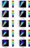 |
Fig. A.2 Density plot in the Pmin − α plane for different values of αmax. For each αmax value we found that α strongly increases with rotation period. The plot in the lower-right corner (αmax = 0.5) demonstrates that our method is limited to αmax < 0.5. Colors are the same as in Fig. 9. |
MAP stands for Maximum A Posteriori which means that the parameters are estimated in a Bayesian way.
Acknowledgments
T.R. acknowledges support from the DFG Graduiertenkolleg 1351 Extrasolar Planets and their Host Stars. A.R. acknowledges financial support from the DFG as a Heisenberg Professor under RE 1664/9-1.
References
- Aerts, C., Christensen-Dalsgaard, J., & Kurtz, D. W. 2010, Asteroseismology (Springer) [Google Scholar]
- Affer, L., Micela, G., Favata, F., & Flaccomio, E. 2012, MNRAS, 424, 11 [NASA ADS] [CrossRef] [Google Scholar]
- Ammler-von Eiff, M., & Reiners, A. 2012, A&A, 542, A116 [NASA ADS] [CrossRef] [EDP Sciences] [Google Scholar]
- Baliunas, S., Sokoloff, D., & Soon, W. 1996, ApJ, 457, L99 [NASA ADS] [CrossRef] [Google Scholar]
- Baliunas, S. L., Hartmann, L., Noyes, R. W., et al. 1983, ApJ, 275, 752 [NASA ADS] [CrossRef] [Google Scholar]
- Balona, L. A. 2011, MNRAS, 415, 1691 [NASA ADS] [CrossRef] [Google Scholar]
- Balona, L. A. 2013, MNRAS, 431, 2240 [NASA ADS] [CrossRef] [Google Scholar]
- Balona, L. A., Guzik, J. A., Uytterhoeven, K., et al. 2011, MNRAS, 415, 3531 [NASA ADS] [CrossRef] [Google Scholar]
- Balona, L. A., Joshi, S., Joshi, Y. C., & Sagar, R. 2013a, MNRAS, 429, 1466 [NASA ADS] [CrossRef] [Google Scholar]
- Balona, L. A., Medupe, T., Abedigamba, O. P., et al. 2013b, MNRAS, 430, 3472 [NASA ADS] [CrossRef] [Google Scholar]
- Baraffe, I., Chabrier, G., Allard, F., & Hauschildt, P. H. 1998, A&A, 337, 403 [NASA ADS] [Google Scholar]
- Barnes, S. A. 2003, ApJ, 586, 464 [NASA ADS] [CrossRef] [Google Scholar]
- Barnes, S. A. 2007, ApJ, 669, 1167 [NASA ADS] [CrossRef] [Google Scholar]
- Barnes, J. R., Collier Cameron, A., Donati, J.-F., et al. 2005, MNRAS, 357, L1 [NASA ADS] [CrossRef] [MathSciNet] [Google Scholar]
- Basri, G., Walkowicz, L. M., Batalha, N., et al. 2010, ApJ, 713, L155 [NASA ADS] [CrossRef] [Google Scholar]
- Basri, G., Walkowicz, L. M., Batalha, N., et al. 2011, AJ, 141, 20 [NASA ADS] [CrossRef] [Google Scholar]
- Bonomo, A. S., & Lanza, A. F. 2012, A&A, 547, A37 [NASA ADS] [CrossRef] [EDP Sciences] [Google Scholar]
- Browning, M. K. 2011, in IAU Symp. 271, eds. N. H. Brummell, A. S. Brun, M. S. Miesch, & Y. Ponty, 69 [Google Scholar]
- Collier Cameron, A. 2007, Astron. Nachr., 328, 1030 [NASA ADS] [CrossRef] [Google Scholar]
- Collier Cameron, A., Donati, J.-F., & Semel, M. 2002, MNRAS, 330, 699 [NASA ADS] [CrossRef] [Google Scholar]
- Covey, K. R., Agüeros, M. A., Lemonias, J. J., et al. 2011, in 16th Cambridge Workshop on Cool Stars, Stellar Systems, and the Sun, eds. C. Johns-Krull, M. K. Browning, & A. A. West, ASP Conf. Ser., 448, 269 [Google Scholar]
- Croll, B., Walker, G. A. H., Kuschnig, R., et al. 2006, ApJ, 648, 607 [NASA ADS] [CrossRef] [Google Scholar]
- Debosscher, J., Blomme, J., Aerts, C., & De Ridder, J. 2011, A&A, 529, A89 [NASA ADS] [CrossRef] [EDP Sciences] [Google Scholar]
- Donahue, R. A., Saar, S. H., & Baliunas, S. L. 1996, ApJ, 466, 384 [NASA ADS] [CrossRef] [Google Scholar]
- Donati, J.-F., & Collier Cameron, A. 1997, MNRAS, 291, 1 [NASA ADS] [CrossRef] [Google Scholar]
- Donati, J.-F., Collier Cameron, A., & Petit, P. 2003, MNRAS, 345, 1187 [NASA ADS] [CrossRef] [Google Scholar]
- Frasca, A., Fröhlich, H.-E., Bonanno, A., et al. 2011, A&A, 532, A81 [NASA ADS] [CrossRef] [EDP Sciences] [Google Scholar]
- Fröhlich, H.-E., Küker, M., Hatzes, A. P., & Strassmeier, K. G. 2009, A&A, 506, 263 [NASA ADS] [CrossRef] [EDP Sciences] [Google Scholar]
- Fröhlich, H.-E., Frasca, A., Catanzaro, G., et al. 2012, A&A, 543, A146 [NASA ADS] [CrossRef] [EDP Sciences] [Google Scholar]
- Gastine, T., Duarte, L., & Wicht, J. 2012, A&A, 546, A19 [NASA ADS] [CrossRef] [EDP Sciences] [Google Scholar]
- Gilliland, R. L., & Fisher, R. 1985, PASP, 97, 285 [NASA ADS] [CrossRef] [Google Scholar]
- Gizon, L., & Solanki, S. K. 2004, Sol. Phys., 220, 169 [NASA ADS] [CrossRef] [Google Scholar]
- Hall, D. S. 1991, in IAU Colloq. 130: The Sun and Cool Stars. Activity, Magnetism, Dynamos, eds. I. Tuominen, D. Moss, & G. Rüdiger, Lect. Notes Phys. (Berlin: Springer Verlag), 380, 353 [Google Scholar]
- Hotta, H., & Yokoyama, T. 2011, ApJ, 740, 12 [NASA ADS] [CrossRef] [Google Scholar]
- Irwin, J., Berta, Z. K., Burke, C. J., et al. 2011, ApJ, 727, 56 [NASA ADS] [CrossRef] [Google Scholar]
- Jester, S., Schneider, D. P., Richards, G. T., et al. 2005, AJ, 130, 873 [NASA ADS] [CrossRef] [Google Scholar]
- Kinemuchi, K., Barclay, T., Fanelli, M., et al. 2012, PASP, 124, 963 [NASA ADS] [CrossRef] [Google Scholar]
- Kiraga, M., & Stepien, K. 2007, Acta Astron., 57, 149 [NASA ADS] [Google Scholar]
- Kitchatinov, L. L. 2005, Phys. Uspekhi, 48, 449 [Google Scholar]
- Kitchatinov, L. L., & Rüdiger, G. 1999, A&A, 344, 911 [NASA ADS] [Google Scholar]
- Küker, M., & Rüdiger, G. 2005a, A&A, 433, 1023 [NASA ADS] [CrossRef] [EDP Sciences] [Google Scholar]
- Küker, M., & Rüdiger, G. 2005b, Astron. Nachr., 326, 265 [NASA ADS] [CrossRef] [Google Scholar]
- Küker, M., & Rüdiger, G. 2007, Astron. Nachr., 328, 1050 [NASA ADS] [CrossRef] [Google Scholar]
- Küker, M., & Rüdiger, G. 2011, Astron. Nachr., 332, 933 [NASA ADS] [CrossRef] [Google Scholar]
- Lanza, A. F., Rodono, M., & Zappala, R. A. 1993, A&A, 269, 351 [NASA ADS] [Google Scholar]
- Marsden, S. C., Jardine, M. M., Ramírez Vélez, J. C., et al. 2011, MNRAS, 413, 1939 [NASA ADS] [CrossRef] [Google Scholar]
- McQuillan, A., Aigrain, S., & Roberts, S. 2012, A&A, 539, A137 [Google Scholar]
- McQuillan, A., Aigrain, S., & Mazeh, T. 2013, MNRAS, 432, 1203 [NASA ADS] [CrossRef] [MathSciNet] [Google Scholar]
- Meibom, S., Barnes, S. A., Latham, D. W., et al. 2011, ApJ, 733, L9 [NASA ADS] [CrossRef] [Google Scholar]
- Morin, J., Donati, J.-F., Forveille, T., et al. 2008, MNRAS, 384, 77 [NASA ADS] [CrossRef] [Google Scholar]
- Morin, J., Donati, J.-F., Petit, P., et al. 2010, MNRAS, 407, 2269 [NASA ADS] [CrossRef] [MathSciNet] [Google Scholar]
- Nielsen, M. B., Gizon, L., Schunker, H., & Karoff, C. 2013, A&A, 557, L10 [NASA ADS] [CrossRef] [EDP Sciences] [Google Scholar]
- Petigura, E. A., & Marcy, G. W. 2012, PASP, 124, 1073 [NASA ADS] [CrossRef] [Google Scholar]
- Reed, B. C. 1998, JRASC, 92, 36 [NASA ADS] [Google Scholar]
- Reiners, A. 2006, A&A, 446, 267 [NASA ADS] [CrossRef] [EDP Sciences] [Google Scholar]
- Reiners, A., & Mohanty, S. 2012, ApJ, 746, 43 [NASA ADS] [CrossRef] [Google Scholar]
- Reiners, A., & Schmitt, J. H. M. M. 2002, A&A, 384, 155 [NASA ADS] [CrossRef] [EDP Sciences] [Google Scholar]
- Reiners, A., & Schmitt, J. H. M. M. 2003, A&A, 398, 647 [NASA ADS] [CrossRef] [EDP Sciences] [Google Scholar]
- Reinhold, T., & Reiners, A. 2013, A&A, 557, A11 [NASA ADS] [CrossRef] [EDP Sciences] [Google Scholar]
- Roettenbacher, R. M., Monnier, J. D., Harmon, R. O., Barclay, T., & Still, M. 2013, ApJ, 767, 60 [NASA ADS] [CrossRef] [Google Scholar]
- Savanov, I. S. 2011a, Astron. Rep., 55, 801 [NASA ADS] [CrossRef] [Google Scholar]
- Savanov, I. S. 2011b, Astron. Rep., 55, 341 [NASA ADS] [CrossRef] [Google Scholar]
- Savanov, I. S., & Dmitrienko, E. S. 2011, Astron. Rep., 55, 890 [NASA ADS] [CrossRef] [Google Scholar]
- Savanov, I. S., & Dmitrienko, E. S. 2012, Astron. Rep., 56, 116 [NASA ADS] [CrossRef] [Google Scholar]
- Schrinner, M., Petitdemange, L., & Dormy, E. 2012, ApJ, 752, 121 [NASA ADS] [CrossRef] [Google Scholar]
- Skumanich, A. 1972, ApJ, 171, 565 [NASA ADS] [CrossRef] [Google Scholar]
- Smith, J. C., Stumpe, M. C., Van Cleve, J. E., et al. 2012, PASP, 124, 1000 [NASA ADS] [CrossRef] [Google Scholar]
- Stumpe, M. C., Smith, J. C., Van Cleve, J. E., et al. 2012, PASP, 124, 985 [NASA ADS] [CrossRef] [Google Scholar]
- Uytterhoeven, K., Moya, A., Grigahcène, A., et al. 2011, A&A, 534, A125 [NASA ADS] [CrossRef] [EDP Sciences] [Google Scholar]
- Walkowicz, L. M., Basri, G. S., & Valenti, J. A. 2013, ApJS, 205, 17 [NASA ADS] [CrossRef] [Google Scholar]
- Zechmeister, M., & Kürster, M. 2009, A&A, 496, 577 [NASA ADS] [CrossRef] [EDP Sciences] [Google Scholar]
All Tables
All Figures
|
Fig. 1 Temperature vs. gravity of all Kepler Q3 stars (black) using KIC parameters. The active sample (Rvar ≥ 0.003) is shown in red. The blue star marks the Sun which is shown for comparison. The dashed line marks log g = 3.5 which was set to exclude giants in the following. |
| In the text | |
|
Fig. 2 Distribution of Rvar for all Kepler Q3 stars. 40 661 active stars lie above the imposed limit Rvar ≥ 0.3% that excludes more than 75% of all stars. |
| In the text | |
|
Fig. 3 Frequency f1 vs. number of zero crossings in Q3. The lower red line equals the number of zero crossings expected for sine-like variations. Stars lying above the upper red line (gray symbols) were discarded because they show more than twice the number of zero crossings expected. |
| In the text | |
|
Fig. 4 Top Panel: light curve and global fit of the star KIC 1995351. Lower Panel (top to bottom): periodograms 1–5. The vertical red lines indicate the highest peak in each periodogram. The periods P1 = 3.24 d and P2 = 3.57 d were selected by our method. |
| In the text | |
|
Fig. 5 Top Panel: light curve and global fit of the star KIC 1869783. Lower Panel (top to bottom): periodograms 1–5. The vertical red lines indicate the highest peak in each periodogram. The periods P1 = 26.2 d and P2 = 20.9 d were selected by our method. |
| In the text | |
|
Fig. 6 Top Panel: light curve and global fit of the star KIC 9580312. Lower Panel (top to bottom): periodograms 1–5. The vertical red lines indicate the highest peak in each periodogram. The periods P1 = 3.97 d and P2 = 4.86 d were selected by our method. |
| In the text | |
|
Fig. 7 Distribution of rotation periods for the 24 124 stars with period P1 and the 18 616 stars with second period P2 with weighted means of 16.3 and 13.3 days, respectively. The distribution of P2 falls off more rapidly towards 30 days because instrumental effects currently hamper the detection of long periods. |
| In the text | |
|
Fig. 8 B − V color vs. rotation period P1 of the 24 124 stars with at least one detected period (gray dots). The filled circles represent data from Baliunas et al. (1996, olive), Kiraga & Stepien (2007, purple), Irwin et al. (2011, red), and McQuillan et al. (2013, blue). Towards cooler stars we found an increase in rotation periods with a steep rise around B − V ≈ 0.6 supplying evidence of rotational braking. The black lines represent a color-period relation found by Barnes (2007) for different isochrones. The four stars mark the position of the Sun (blue), KIC 1995351 (cyan), KIC 1869783 (purple), and KIC 9580312 (red) for comparison. |
| In the text | |
|
Fig. 9 Density plot of rotation periods P1 vs. Rvar with bright regions representing a high density, whereas dark regions express low density. The annotation of the color bar contains the total number of stars in each bin. The distribution shows that the range increases towards shorter periods. Since fast rotators are expected to exhibit an enhanced level of activity, the range could probably be used as proxy for stellar activity. |
| In the text | |
|
Fig. 10 Distribution of ages inferred from rotation periods P1 for different color bins. For B − V > 1.0 (red and blue) we found a bimodal distribution in agreement with McQuillan et al. (2013). The dashed black and red lines show uniform age distributions (on a logarithmic scale). |
| In the text | |
|
Fig. 11 Rotation period Pmin vs. α for all stars with two detected periods. The colors represent different temperature bins, the dashed black line marks the detection limit. The relative shear α grows towards longer rotation periods. More than 75% of all stars with detected period P1 exhibit a second period P2, and lie above the detection limit. This trend cannot be broken by the 5505 stars with only one detected period, because most of the missing stars lie above the upper limit αmax = 0.3. |
| In the text | |
|
Fig. 12 Effective temperature vs. relative shear α. We found that α slightly increases towards cooler stars. The colors indicate different variability ranges. A distinct correlation between α and the range is only visible for the stars with very high ranges Rvar > 5%. These stars group at small α values over a large temperature range. Low α represents short periods, probably indicating that their young age. |
| In the text | |
|
Fig. 13 Rotation period Pmin vs. absolute shear ΔΩ. The colors are the same as in Fig. 11, the detection limit is marked by the horizontal dashed line, and the diagonal dashed lines mark the upper and lower limit αmax and αmin, respectively. We found that ΔΩ is independent of Pmin over a large period range, although the upper and lower limit suggest an increase of ΔΩ towards short periods, showing large scatter on one order of magnitude. |
| In the text | |
|
Fig. 14 Density plot in the Pmin − ΔΩ plane. For ΔΩ < 0.10 rad d-1 the total shear does not depend on rotation period. For ΔΩ > 0.10 rad d-1 we found large scatter of ΔΩ from fast to moderate rotators. |
| In the text | |
|
Fig. 15 Effective temperature vs. horizontal shear ΔΩ summarizing different measurements: the olive diamonds and error bars were taken from Barnes et al. (2005), the olive dashed curve from Collier Cameron (2007). Orange diamonds and error bars show measurements from Ammler-von Eiff & Reiners (2012). Our measurements are shown as gray dots. The red dash-dotted line and the light blue dashed line show theoretical predictions from Küker & Rüdiger (2011). The black dashed line marks our detection limit. The four stars mark the positions of the Sun (blue), KIC 1995351 (cyan), KIC 1869783 (purple), and KIC 9580312 (red) for comparison. The vertical red bar indicates stars hotter than 7000 K with probable large contamination of pulsators. The open black circles represent weighted means of our measurements for different temperature bins. From 3500−6000 K, ΔΩ shows only weak dependence on temperature. Above 6000 K the shear strongly increases as reported by Barnes et al. (2005) and Collier Cameron (2007). The different behavior of ΔΩ in these two temperature regions was supported by theoretical predictions from Küker & Rüdiger (2011, red and light blue lines). |
| In the text | |
|
Fig. 16 Comparison of periods from Nielsen et al. (2013, left panel) and McQuillan et al. (2013, right panel) with the periods P1 from Fig. 8. We found good agreement with both samples, although the auto-correlation method from McQuillan et al. (2013) was less prone to alias periods than our method, as is obvious from the missing peak around 0.5 in the right panel. |
| In the text | |
|
Fig. A.1 Density plot in the Teff − α plane for different values of αmax. For each αmax value we found that α slightly increases towards cooler stars. The plot in the lower-right corner (αmax = 0.5) demonstrates that our method is limited to αmax < 0.5. Colors are the same as in Fig. 9. |
| In the text | |
|
Fig. A.2 Density plot in the Pmin − α plane for different values of αmax. For each αmax value we found that α strongly increases with rotation period. The plot in the lower-right corner (αmax = 0.5) demonstrates that our method is limited to αmax < 0.5. Colors are the same as in Fig. 9. |
| In the text | |
Current usage metrics show cumulative count of Article Views (full-text article views including HTML views, PDF and ePub downloads, according to the available data) and Abstracts Views on Vision4Press platform.
Data correspond to usage on the plateform after 2015. The current usage metrics is available 48-96 hours after online publication and is updated daily on week days.
Initial download of the metrics may take a while.