| Issue |
A&A
Volume 559, November 2013
|
|
|---|---|---|
| Article Number | A49 | |
| Number of page(s) | 9 | |
| Section | Interstellar and circumstellar matter | |
| DOI | https://doi.org/10.1051/0004-6361/201321453 | |
| Published online | 11 November 2013 | |
CO2 formation on interstellar dust grains: a detailed study of the barrier of the CO + O channel
1 LERMA, UMR8112 du CNRS, de l’Observatoire de Paris et de l’Université de Cergy Pontoise, 5 mail Gay Lussac, 95000 Cergy Pontoise Cedex, France
e-mail: This email address is being protected from spambots. You need JavaScript enabled to view it.
2 Dipartimento di Fisica ed Astronomia, Universitá degli Studi di Catania, via Santa Sofia 64, 95123 Catania, Italy
Received: 12 March 2013
Accepted: 5 September 2013
Abstract
Context. The formation of carbon dioxide in quiescent regions of molecular clouds has not yet been fully understood, even though CO2 is one of the most abundant species in interstellar ices.
Aims. CO2 formation is studied via oxidation of CO molecules on cold surfaces under conditions close to those encountered in quiescent molecular clouds.
Methods. Carbon monoxide and oxygen atoms are codeposited using two differentially pumped beam lines on two different surfaces (amorphous water ice or oxydized graphite) held at given temperatures between 10 and 60 K. The products are probed via mass spectroscopy by using the temperature-programmed desorption technique.
Results. We show that the reaction CO + O can form carbon dioxide in solid phase with an efficiency that depends on the temperature of the surface. The activation barrier for the reaction, based on modelling results, is estimated to be in the range of 780−475 K/kb. Our model also allows us to distinguish the mechanisms (Eley Rideal or Langmuir-Hinshelwood) at play in different temperature regimes. Our results suggest that competition between CO2 formation via CO + O and other surface reactions of O is a key factor in the yields of CO2 obtained experimentally.
Conclusions. CO2 can be formed by the CO + O reaction on cold surfaces via processes that mimic carbon dioxide formation in the interstellar medium. Astrophysically, the presence of CO2 in quiescent molecular clouds could be explained by the reaction CO + O occurring on interstellar dust grains.
Key words: publications, bibliography / astrochemistry / atomic processes / ISM: abundances / ISM: atoms / ISM: molecules
© ESO, 2013
1. Introduction
Carbon dioxide has already been detected in the interstellar medium (ISM) by d’Hendecourt & Jourdain de Muizon already few decades ago (1989). It represents one of the most common and abundant types of ices, and many astronomical observations (by the Infrared Space Observatory and the Spitzer Space Telescope) confirm the presence of CO2 in different environments, such as Galactic-centre sources (de Graauw et al. 1996), massive protostars (Gerakines et al. 1999; Gibb et al. 2004), low-mass young stellar objects (Nummelin et al. 2001; Aikawa et al. 2012), brown dwarfs (Tsuji et al. 2011) background stars (Knez et al. 2005), in other galaxies (Shimonishi et al. 2010; Oliveira et al. 2011), and in comets (Ootsubo et al. 2010). CO2 is predicted to have low abundance in the gas phase (NCO2/NH2 = 6.3 × 10⁻¹¹; Herbst & Leung 1986), and this is confirmed by observations (van Dishoeck et al. 1996). Low abundances in gas phase, together with its observed high abundances in the solid phase, cannot be explained exclusively by formation via gas-phase schemes (Hasegawa et al. 1992), therefore surface reactions are evoked to justify a high abundance of carbon dioxide ices.
Extensive experimental studies have been carried out to study formation routes of CO2 formation in solid-phase. Energetic routes, such as irradiation of CO ices (pure or mixed with H2O) with photons, charged particles or electrons, have been investigated by Gerakines et al. (1996), Palumbo et al. (1998), Jamieson et al. (2006), Ioppolo et al. (2009), and Laffon et al. (2010), and have shown an efficient formation of carbon dioxide. Whittet et al. (1998), however, provided the evidence of efficient CO2 formation in quiescent dark clouds towards the line of sight Elias 16. This suggests that the presence of CO2 in grain mantles can also be explained through chemical pathways occurring without the addition of energy and where the radicals are thermalized with the surface. Two of these pathways are
- 1.
CO + OH → CO2 + H
- 2.
CO + O → CO2.
In recent experimental studies it has clearly been shown that reaction 1 leads to CO2 formation, although no consistent results were obtained concerning the activation barrier: little or barrierless in Oba et al. (2011) and “high” (400 K) in Noble et al. (2011). Reaction 2 has been studied theoretically (Talbi et al. 2006; Goumans et al. 2008), and those studies suggest there is a high activation barrier (2500−3000 K). The first successful laboratory investigation of the formation of CO2 by non-energetic processes was performed by Roser et al. (2001), who studied the surface reaction of CO and O atoms. In a first set of experiments they co-deposited the two species at 5K and performed a temperature-programmed desorption (TPD). Probably due to the low sensitivity of the quadrupole mass spectrometer they were using at that time, they did not detect any CO2 formation. To prove the formation of carbon dioxide through such a pathway and to give a first estimate of the barrier for such a reaction they subsequently devised an experiment in which the co-deposited layer of CO and O atoms was covered by a layer of porous water ice. The TPD performed in such conditions allowed the formation of CO2 to be detected thanks to the reaction of CO and O migrating in the interconnected pores of the amorphous ice. Under the hypothesis that the mobility of species stemmed from thermally activated processes, a reaction barrier of 290 K was obtained that explained the formation of carbon dioxide even in quiescent clouds1. Raut & Baragiola (2011) confirmed the formation of CO2 by Roser et al. (2011). They performed experiments showing the formation of small amounts CO2 during co-deposition of CO and cooled O and O2 at 20 K, although they did not provide any activation barrier for reaction 2. Here we present further experimental studies of reaction 2. CO2 production on cold surfaces (10−40 K) was investigated by concurrent exposures of CO molecules and O atoms. The CO + O reaction is studied in a submonolayer regime on two different substrates: amorphous solid water (ASW) ice and oxidized graphite. As previously found in Raut & Baragiola (2011), CO2 formation is in competition with O2 and O3 formation via the O + O and O2 + O reaction routes. We also determined an activation energy of the CO + O reaction and the physical chemical mechanisms occurring on the surface by developing a kinetic model.
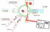 |
Fig. 1 Schematic top-view of the FORMOLISM setup and the FT-RAIRS facility. |
2. Experiments
The experiments were performed with the FORMOLISM (FORmation of MOLecules in the InterStellar Medium) set-up (Fig. 1), which is described elsewhere (Amiaud et al. 2006; Congiu et al. 2012). The set-up is dedicated to investigating physical chemical reactions on surfaces of astrophysical interest, under conditions roughly similar to those encountered in the ISM. Experiments take place in an ultra-high vacuum chamber (base pressure 10-10 − 10-11 mbar) containing a graphitic sample surface (0.9 cm in diameter), operating at temperatures between 10 and 400 K. The temperature is controlled by a calibrated silicon-diode sensor and a thermocouple (AuFe/Chromel K-type) clamped on the sample holder. The system is equipped with a quadrupole mass spectrometer (QMS), which is used for temperature-programmed desorption (TPD) experiments. ASW ice is grown in situ on the graphite sample. The H2O vapour is obtained from deionized water previously purified by several freeze-pump-thaw cycles carried out in a vacuum. H2O molecules are deposited on the surface maintained at 110 K through a leak valve equipped with a micro channel doser positioned at 3.5 cm in front of the cold surface during the water ice deposition phase. The 13CO molecules and O atoms are sent simultaneously (co-deposition) on the surface via two triply differentially pumped beam lines. We used 13CO instead of 12CO to increase the signal-to-noise ratio of the mass signal of the CO reactant and the final CO2 product. Hereafter we refer to 13CO as CO. The O atoms are produced by dissociation of O2 molecules. The two beam lines are equipped with microwave dissociation sources (surfatron cavities delivering 200 W at 2.45 GHz) that can generate atoms by breaking molecular internal bonds. With the microwave source turned on, the dissociation efficiency of O2 was τ = 73 ± 5% at the time of the experiments performed on ASW and 61 ± 7% when we perfomed the experiments on graphite2. Atoms and undissociated molecules are cooled and instantaneously thermalized upon surface impact with the walls of the quartz tube.
We have calibrated the molecular beam as described in Amiaud et al. (2007) and Noble et al. (2012) and found that the first monolayer (1 ML = 1015 molecules cm-2) of both 13CO and O2 was reached after an exposure time of about six minutes, which therefore gives a flux φO2off,CO = (3.0 ± 0.3) × 1012 molecules cm-2 s-1. Once the O2 discharge is turned on, the O-atom flux is φO = 2τφO2off = 5.4 × 10¹² atoms cm-2 s-1 and the O2 flux φO2on = (1 − τ) φO2off = 1012 molecules cm-2 s-1. In addition, we determined that the beam did not contain O or O2 in an excited state by tuning the ionizing electron energy inside the QMS head as described in Congiu et al. (2009).
CO2 formation was investigated on two different surfaces, ASW and oxidized graphite. Fixed doses of O (+O2), 0.5 ML, and CO, 0.5 ML, were deposited on the surface held at a given constant temperature. After each deposition, the surface was heated with a linear temperature ramp of 10 K/min until the adsorbate had fully desorbed from the surface (around 90−95 K). The surface was then cooled again so that a new deposition could begin at a different temperature. For both substrates (ASW ice and graphite), we used eight surface temperatures (10, 20, 30, 35, 40, 45, 50, 60 K).
We also performed an experiment to check the CO reactivity with O2 and O3 to form CO2. For this purpose, we performed two sets of TPD experiments. First, the CO + O2 reaction was checked with a set of experiments consisting of three different depositions – each one followed by TPD – with the surface temperature held at 10 K: 2 ML of CO + 2 ML of O2 and the co-deposition of 2 ML CO and O2. The CO + O3 reaction was studied through a similar set of experiments except that we had previously produced ozone via the O + O2 reaction occurring on the surface, eliminated the residual O2 by heating to 50 K, and only then, deposited CO at 10 K.
3. Experimental results
From an energetic point of view, oxidation of CO to form carbon dioxide may proceed by the following reactions:
- 1a.
CO + O → CO2 (− ΔH = 532 kJ/mol)
- 2a.
CO + O2 → CO2 + O (− ΔH = 33 kJ/mol)
- 3a.
CO + O3 → CO2 + O2 (− ΔH = 425 kJ/mol) 3.
To disentangle which of these reactions are effectively able to produce CO2 on cold surfaces, we have to be sure that CO2 is really formed on the surface and that it is not present as an impurity in the CO bottle. To check this possibility, we have performed further experiments. In Fig. 2 we show one of these tests where we checked the CO2 presence on the graphite surface – held at 10 K – after an exposure of 4 ML of CO and after 4 ML of CO + O. The difference between the two TPDs is evident, and comparing the two CO2 signals we find CO2(CO dep)/CO2(CO + O dep) ~ 8%, which confirms that the majority of the CO2 detected is formed through surface reactions.
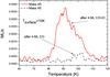 |
Fig. 2 TPD curves of mass 45 (13CO2) between 60 and 120 K after 4 ML of 13CO exposure (dotted curve), and after 4 ML of 13CO + O (solid line) on graphite held at 10 K. |
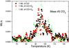 |
Fig. 3 TPD curves of mass 45 (13CO2) between 65 and 125 K after deposition of 1 ML of 13CO (squares), 13CO + O2 (circles) and 13CO + O3 (triangles) on graphite held at 10 K. |
Roser et al. (2001) and Raut & Baragiola (2011) have already studied reaction 1a, showing that this reaction can produce carbon dioxide without the intervention of energetic processes. As for reaction 2a, Mallard et al. (1994) suggested a very high activation energy barrier (~24 000 K), while reaction 3a, to the best of our knowledge, has not been studied yet. In our experimental set-up, the oxygen atom beam is produced through dissociation of O2 molecules with a dissociation fraction which never exceeds 80%. This means that we always have an O2 “pollution”. Moreover, when O atoms arrive on the surface, they efficiently recombine to form O2 and O3 (Minissale et al. 2013).
For these reasons, it is not possible to study reaction 1a without knowing how (and if) reaction 2a and 3a work. Figure 3 shows three TPD spectra of mass 45 after deposition on oxidized graphite held at 10 K of 1 ML CO, co-deposition of 1 ML CO + O2, and 1 ML CO + O3. The three TPD curves and integrated areas of the curves are very similar and this suggests that the CO + O2 reaction does not occur or that at least it is very inefficient at producing CO2 in accord with Mallard et al. (1994). We have another indication of the CO + O2 inefficiency by comparing the area of the CO peak with and without O2. In the two cases we do not detect any measurable variations of the CO yield. We get to the same conclusion as far as the CO + O3 reaction is concerned. No difference can be appreciated in the comparison between the peak area of CO, of background CO2 and of O3. This indicates that CO + O3 is not a fast reaction to produce CO2 either.
In Fig. 4 we show the TPD traces resulting from irradiating ASW ice held at 20 K with 0.5 ML of CO + O (i.e., 0.5 ML CO, 0.15 ML O2, 0.7 ML O). Four main peaks appear at masses 29, 32, and 45. The mass-29 peak is clearly due to the CO desorption, which occurs between 32 K and 55 K and peaks at 41 K. Mass 32 presents two peaks, the first one between 28 and 42 K – peaked at 34 K – is due to O2 desorption while the second one peaking at around 65 K included between 55 K and 75 K is due to the desorption of O3 detected in the form of O fragments, as a result of the O3 cracking in the head of the QMS. We are certain that this peak comes from O3 desorption because we also detect the signal at mass 48, which has the same shape, though less intense, of the one at mass 32 in the same temperature range (not shown). Finally, the tiny high-temperature peak also shown in the insert comes from to the CO2 desorption occurring between 75 and 95 K and peaking at 83 K.
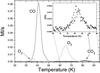 |
Fig. 4 TPD curves at mass 29, 32, and 45 after irradiation of 0.5 ML of 13CO + O on ASW ice held at 20 K. Four peaks are visible. The first peak between 28 K and 42 K is due to O2 desorption, the second one between 32 and 55 K is due to 13CO desorption. The third peak between 55 K and 75 K represents O3 desorption, while the high-temperature peak is the desorption of 13CO2 (75−95 K). |
The results of the other set of experiments are very similar to the one just described. In fact, we observe always four peaks (except for the 50 K experiment, where O2 has already desorbed before starting the TPD), but their intensities change with temperature as shown below. Figure 4 indicates that two molecules are actually formed on the surface, O3 and CO2. Moreover, O2 can also be either formed on the surface via the O + O reaction or come from the beam because of the non-total dissociation of O2 molecules. Considering all reactants and products and remembering that reactions 2a and 3a can be disregarded, the possible reactions occurring on the surface are listed below:
- 1a.
CO + O → CO2
- 4a.
O + O → O2
- 5a.
O + O2 → O3
- 6a.
O + O3 → 2 O2.
The last three reactions were studied in Minissale et al. (2013). While reactions 4a and 5a seem to be barrier-less (or with a very low activation barrier below 190 K/kb), reaction 6a does not occur and is likely to have a high activation barrier (see Table 1).
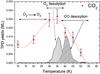 |
Fig. 5 13CO2 yield as a function of surface temperature during deposition of 0.5 ML of 13CO + O. Circles represent the integrated area under the TPD curves of mass 45 after a deposition of 0.5 ML of 13CO + O on ASW ice held at different temperatures (10 K, 20 K, 30 K, 35 K, 40 K, 45 K, 50 K, 60 K). The solid line is a fit of the area behaviour. The TPD peaks (obtained at Tsurface = 20 K) added in the figure show when O2 and 13CO desorb, and this helps interpret the 13CO2 yield behaviour with temperature. |
List of surface reactions with the respective activation barriers.
Apparently, reaction 1a is in competition with reactions 4a and 5a. To understand how efficiently the CO + O reaction proceeds and to derive its activation barrier, we performed several experiments at a fixed coverage and by varying the surface temperature. Temperature, in fact, affects both oxygen atom diffusion and the desorption of species and these two processes give us the key to understand our results (Figs. 5 and 6) and consequently the way CO2 is formed.
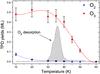 |
Fig. 6 O2 and O3 yields as a function of surface temperature during deposition of 0.5 ML of 13CO + O. The circles and the squares represent the integrated area under the TPD curves of O2 and O3, respectively, after deposition of 0.5 ML of 13CO + O on ASW ice held a different temperatures (10 K, 20 K, 30 K, 35 K, 40 K, 45 K, 50 K, 60 K). The solid line is a fit of the area behaviour. The added O2 TPD (obtained at Tsurface = 20 K) helps interpret the O3 yield behaviour with temperature. |
As we can see in Fig. 5, the CO2 signal is already present at 10 K4, and it reaches a maximum when the surface temperature during exposure is 35 K. Subsequently, for higher temperatures the CO2 signal decreases and becomes zero at 60 K. This behaviour can be explained by considering three different “temperature zones”: below 30 K, between 30 K and 35 K, and higher than 35 K. In the range between 10 K and 30 K, the majority of oxygen atoms are used to produce ozone (Fig. 6) via reaction 4a and 5a, and its production rises with temperature owing to the increase in O diffusion. In this low-temperature zone, only a small amount of oxygen atoms is used to produce CO2, probably via the Eley-Rideal mechanism, see below. When O2 starts to desorb (mid-temperature zone, 30−35 K) O atoms have a lower probability of meeting O2 molecules to form O3. In fact, we see a decrease in the amount of O3 desorbed (Fig. 6), while in this range of temperature the probability that an oxygen atom encounters a CO molecule increases (as a consequence of the reduced coverage of O2). At temperatures higher than 35 K, CO desorption begins and the CO2 signal begins to drop with same pattern observed for ozone. This suggests that also at high temperatures (45−50 K) molecules and atoms coming from the beam still have a residence time on the surface long enough to react and form appreciable amounts of ozone and CO2. The shape of the CO2 and O3 yields in Figs. 5 and 6 suggest that CO2 formation is limited by O2 molecules or, in other words, that reaction 1a is in competition with reactions 4a and 5a. In fact, only when the O3 signal decreases (and O2 desorbs) CO2 formation rises. However, presence of O2 apart, CO2 always forms in small amounts, and this very probably indicates the existence of an activation barrier (hereafter Ea) for the reaction CO + O. To evaluate Ea and to understand what surface mechanisms are responsible for CO2 formation we have developed a model described in the next section.
4. Model
In this section we present the model used to fit our experimental data. It is composed of two sets of differential equations. Reactions 1a, 4a, and 5a can occur through two mechanisms: the Eley-Rideal (ER) and the Langmuir-Hinshelwood (LH) mechanisms. In the ER mechanism one molecule is already adsorbed on the surface and the other comes from the gas phase (i.e., the beam line). In the LH mechanism, both molecules are bound to the surface and by diffusion they can meet each other and react. We consider five species: two are coming exclusively from the beam, O atoms and CO molecules, two are formed only on the surface, O3 and CO2, and one, O2, is coming both from the beam and formed on the surface. Below the list of equations governing the CO2 formation by the ER mechanism follows: 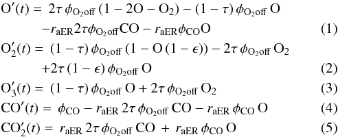 where capital-element symbols express the surface densities (expressed in fraction of ML) of the species, τ is the dissociated fraction of O2 defined in Sect. 2, φO2off,CO are the fluxes (0.003 cm-2 s-1) of O2 and CO respectively, raER is the reaction probability of CO + O via ER, and ϵ is the evaporation probability – due to chemical desorption – of O2 formed on the surface. Simple calculations give that 2τφO2off and (1 − τ)φO2off are the O and O2 flux respectively when the discharge is on. Similarly, as for the CO2 formation by the LH mechanism, we have:
 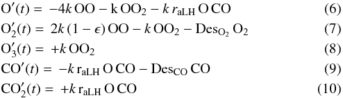 where capital element symbols express the surface densities (expressed in ML) of the species, k is the diffusion coefficient of O atoms (the unit of k is ML-1 s-1, that can be transformed in the usual unit cm2 s-1 by considering that 1 ML = 1015 molecules cm-2), raLH has the same physical meaning of raER, but in the case of LH reactions, DesO2,CO are functions that take into account O2 and CO desorption. These two functions are expressed through the first-order Polanyi-Wigner equation
  (11)where ν is the “attempt frequency” (s-1) for overcoming the barrier to desorption, and EO2,CO are the activation energies for desorption of O2 and CO respectively. Our experimental data provide the fraction of ML of each species present on the surface, therefore in this two sets of equation we have six free parameters: raER,LH, EO2,CO, ϵ and k. Actually, four of these parameters have already been studied under very similar experimental conditions (ϵ in Dulieu et al. 2013; k in Minissale et al. 2013, EO2,CO in Noble et al. 2012), hence by using their measured values we can reduce to two the number of free parameters, namely, raER, and raLH; ϵ is equal to zero in the case of a water ice surface while it is 0.5 if the experiments are carried out on graphite. The diffusion coefficient k is a function of the temperature and we describe it using the law k = k0(1 +
  ), where k0 is 0.9 and T0 is 10 K. Finally, the EO2 and ECO desorption barriers are two energy distributions centred at 1310 K/kb and 1430 K/kb respectively. In our model, we could have added another couple of parameters, kO2,CO, representing the O2 and CO diffusion. However, O diffusion is always dominant with respect to O2 or CO diffusion. The addition of O2 and CO diffusion would cause a quicker consumption of O atoms, without significant changes of the final amount of species. Introducing two more free parameters would then be of secondary importance for the purpose of this work and it would add more complexity. For these reasons we have chosen to neglect the diffusion of O2 and CO.
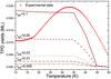 |
Fig. 7 Model results for CO2 production on ASW (pure ER). The curves in this figure were obtained by using rLH = 0, and different rER values (ranging from 0.005 to 0.1). The squares are a best fit of the experimental values. |
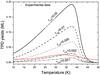 |
Fig. 8 Model results for CO2 production on ASW (pure LH). The curves in this figure were obtained by using rER = 0, and different rLH values (ranging from 0.001 to 0.02). The squares are a best fit of the experimental values. |
Model results showing carbon dioxide yields as a function of surface temperature.
To find the best fit of our experimental values, we have proceeded in this way: we set one of the two parameters to zero and vary the other between 0 and 1. We thus find a value that reproduces the experimental CO2 yield at 10 K and that at once does not overcome the other experimental CO2 yields. This value will be an upper limit. In the case of raER, a value higher than 0.05 returns too much CO2 (Fig. 7) while in the case of raLH, the upper limit is around 0.002 (Fig. 8). Then, through the χ2 test – here we compare the simulated outcome to the experimental values – we have found that the best couple of reaction probabilities is raER = 0.021 and raLH = 0.0019. The model results showing the yields of all species are displayed in Fig. 9. To find acceptable solutions we need concentrate on the CO2 curve. In fact, the reaction probabilities are the only free parameters of our model and one small variation of them strongly affects the CO2 curve (ra appears in each term of the CO2 equations), that is why the experimental CO2 yields are the most important constraints in our model. Moreover, the model allows us to distinguish and quantify the contribution to CO2 formation by either ER or LH mechanism.
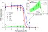 |
Fig. 9 Model results for all species on ASW. The curves in this figure were obtained by using rLH = 0.0019 ± 0.0005 and rER = 0.021 ± 0.007. The circles, stars, triangles and squares represent O2, CO2, CO, and O3 experimental results respectively. The inset displays a magnified view of the CO2 yield around its maximum for clarity. |
In Fig. 10 we show the individual contributions to CO2 formation by ER or LH mechanism as a function of surface temperature. In Table 2 the CO2 yield is expressed in monolayers, in units of the normalized amount formed at 10 K, and in fractions of the total carbon dioxide formed. CO2 formation via ER mechanism appears to be constant with temperature between 10 and 40 K also because, in theory, this mechanism is temperature independent. At higher surface temperatures, however, ER starts to be inefficient because of the desorption and the decrease of the residence time of species on the surface, thus the CO2 production efficiency by this mechanism drops off. On the contrary, the LH mechanism depends on the surface temperature and its efficiency increases going from 10 to 40 K owing to the favoured diffusion of atoms. Beyond 40 K, as occurs for the ER case, the probability that O atoms and CO molecules leave the surface is high and the CO2 yield decreases fast with temperature. The ER and LH contribution to CO2 formation is approximately equal at low temperatures (below 20 K), while at high temperatures most CO2 is formed via the LH mechanism. This is not surprising considering the power law dependence on the temperature of the diffusion parameter.
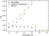 |
Fig. 10 Model results showing the contribution to CO2 formation by either ER (triangles) or LH (circles) mechanism. Contributions to CO2 formation are expressed in monolayers (ML) as a function of surface temperature. |
4.1. Evaluation of the CO + O barrier
The two reaction probabilities raER and raLH give the probability that the CO + O reaction occurs, thus they have the same physical meaning and can be used to evaluate other physical quantities. By inverting a normalized Arrhenius equation the desorption energy Ea can be calculated as follows:  (12)Two alternative strategies can be used to evaluate the activation barrier of the reaction; we can derive the reaction barrier Ea either from raER or raLH.
4.1.1. ER case
In collision theory, this law is derived by considering gas phase particles described through a Maxwell-Boltzmann (MB) energy distribution and assuming that the interactions between the reactants can occur only via head-on collisions (see Atkins 2006). For ER reactions, the use of Eq. (12) is plausible because the interactions occur between a particle coming from the gas phase (MB distribution) and a particle thermalized with the surface. In this case, somehow similarly to gas phase reactions, the impinging particles either collide and react with one adsorbate or have enough energy to hop on the surface before thermalizing and accommodating in an empty adsorption site. Gas phase molecules coming from the beam-line are at around Tgas = 300 ± 20 K/kb while the target particles adsorbed on the substrate are thermalized with the surface at Tsolid = 10 − 60 K/kb. The temperature in Eq. (12) represents the average molecular (atomic) kinetic energy ( ) and in a gas at the thermodynamic equilibrum, is proportional to the thermodynamic temperature. The problem is to know the exact temperature (Teff) to insert in Eq. (12). We consider three different cases:
-
 K
K -
 K.
K. -
 K.
K.
Evidently, we do not take into account the case Teff = Tsolid, because that means to consider molecules already thermalized with the surface, as in a pure LH process.
In the first case (T = Tg = 300 K) we obtain a barrier of 1200 K/kb. Clearly, in our experiments we cannot consider CO and O as two gases at the same thermodynamic equilibrium so the temperature is likely to be lower than 300 K. This means that Ea = 1200 K/kb is to be considered only an upper limit of the activation barrier.
The second and third cases are Teff = 202, 123 K. This choice is justified by the equation below5 (13)where μ is the effective mass of the CO and O system. These temperatures correspond to the velocity of the centre of mass of the system. By substituting their values in Eq. (12), we find a CO + O reaction barrier between EaER = 780–475 K/kb.
4.1.2. LH case
As stated above, we have also tried to derive the reaction barrier from raLH.
In general, the activation barrier of a process or reaction is the same independently of the mechanism that led to it. As to the LH mechanism, reaction partners adsorbed in the same site collide at the temperature (velocity) of the substrate; the disadvantage with respect to overcoming the barrier in the ER case is the lower energy of the colliding partners, but with the advantage that they will collide ν times per second (usually ν = 1012 − 13 s-1) instead of only once.
It should be noted that rLH is dependent on the temperature even though we have given a unique value of the reaction probabilities6. The temperature dependence of rLH is not as simple as in the Arrhenius case (Eq. (12)). In addition, it cannot be derived from the experimental values because they do not provide enough constraints, hence we give a mean value  across the whole temperature range investigated (10−60 K). We then try to estimate the reaction barrier by taking into account the two following considerations:
-
i)
although O-atoms diffusion is predominant with respect to that of O2 and CO, at high temperatures7 also O2 and CO diffusion has to be taken into account if a proper evaluation of rLH(T) is required.
-
ii)
Non-exponential behaviour of the CO2 formation rate due to occurrence of tunneling at very low temperatures (Goumans & Andersson 2010, see Fig. 11).
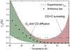
Fig. 11 Temperature dependence of rLH(T) between 10 and 60 K. The two pinstriped regions indicate how a different parametrization of tunneling for CO + O reaction and of O2 and CO diffusion can change our estimation of rLH(T). The dashed line represents our experimental data. Full circles are an example of a pure Arrhenius behaviour.
These considerations suggest that rLH(T), for T < 25 K, is better described by this law  (14)where rtunn(Ea,T) (it is ≥0) represents the rate of tunneling of the CO + O reaction and it is able to increase the reaction probabilities value at low temperature. By inverting Eq. (14) we have
  (15)By putting Teff = 25 K in Eq. (15), rLH(25 K) = 0.0019 and rtunn(Ea,T) = 0, thus and we obtain a lower limit for Ea of 160 K/kb. This value is underestimated for two reasons:
-
At 25 K the tunneling term could become to be dominant with respect to the classical one (Arrhenius law), and clearly is not zero.
 is a mean value, and very probably rLH(T) presents a minimum around 25 K.
This means that rLH(25 K) ≪ 0.0019 and Ea ≫ 160 K/kb are consistent with the values obtained for rER.
4.1.3. Conclusions
We have described above how we evaluated the activation barrier of the CO + O reaction. Our model allows us to distinguish which mechanisms (Eley Rideal or Langmuir-Hinshelwood) is at play in different temperature regimes and we are able to give a range of values of the activation barrier of reaction CO + O of 780−475 K/kb (see Table 3). We have to note that these values make sense only in the range of validity of Eq. (12). Our results are summarized in Table 3. Finallly, it should be noted that the range of activation energy barriers given in this work are only apparently inconsistent with the 290 K/kb value of Roser et al. 2001, which can actually be considered one of the diverse cases addressed in the present paper. In fact, they provide an estimation (not a measure) of the barrier by using only the classical LH mechanism (very low Teff) (on the other hand the ER mechanism (high Teff) with the same barrier would produce more CO2 than that they observed.). Their estimate can thus be considered a lower limit of the barrier which is included in our study of the LH case (lower limit =160 K/kb).
Activation barrier.
5. Astrophysical conclusions
In this paper we have shown that CO2 can be formed by the CO + O reaction on cold surfaces, such as amorphous water or oxidized graphite. This reaction is relevant to astrochemistry in that it may explain CO2 formation on interstellar dust grains by surface reactions and thus justifies its abundance in the solid phase. As mentioned in the introduction, the CO + O reaction competes with the CO + OH reaction (some experimental works have already been conducted by Ioppolo et al. 2013), another non-energetic route to CO2 formation in space. The CO + OH pathway seems to be facilitated by the low barrier of the reaction, but it has an other type of hindrance. In fact, it requires OH formation first (see Chaabouni et al. 2012; Cuppen et al. 2010, and references therein for details on OH formation in space). In H-rich environments, OH can be formed easily, although it can be very quickly destroyed to form water. These facts suggest that the CO2(CO + O)/CO2(CO + OH) ratio strongly depends on three parameters:
-
the O/H ratio, very probably the most important parameter;
-
the grain temperature: the higher it is the shorter is the H residence time on the grain and thus the probability of OH formation;
-
H and O diffusion on the surface: since only the first one is usually considered in models (e.g., Garrod & Pauly 2011), the CO + O contribution is, in our opinion, underestimated.
In conclusion, the CO + O pathway seems to be important in those astrophysical environments where a lack of UV photons forbids the energetic routes leading to CO2 or in environments with large abundances of atomic oxygen. Although the abundance of O atoms in ISM remains controversial, the detected high abundances of solid CO2 together with observations of atomic oxygen in the molecular cloud Taurus8 (Whittet et al. 1998), Sgr B2, and L1689N29 (Charnley & Kaufman 2000; Caux et al. 2001), make these environments a good example of where the CO + O reaction can efficiently proceed to form CO2.
Nevertheless we notice that the experimental conditions were not completely consistent with physical chemical conditions of quiescent molecular clouds.
τ represents the percentage of O2 molecules dissociated, which also defines the O/O2 ratio in the beamline; e.g., every 10 O2 molecules, if τ is 0.7, we will have 14 O atoms and 3 O2 molecules.
NIST Chemistry WebBook.
We know indirectly that CO2 is formed at deposition temperature, namely, before the TPD. We do not see, in fact, any change in the RAIR spectra of O3 during the TPD. This means that all O atoms are able to scan the surface, hence to react at deposition temperature (see Minissale et al. 2013, for more details).
See Appendix A.
This is also true for what concerns the ER mechanism although the variation of rER with temperature is a minor effect. The uncertainty due to this effect is accounted for by the error bar of the activation barrier.
The onsets of O2 and CO diffusion take place at 25 K and 30 K, respectively.
Taurus is a quiescent dark cloud where CO2 formation cannot be explained through energetic formation routes.
Sgr B2 is a giant molecular cloud and L1689N where large amounts of atomic oxygen were observed (Lis et al. 2001; Caux et al. 2001).
Acknowledgments
The LERMA-LAMAp team in Cergy acknowledges the support of the national PCMI programme founded by CNRS, the Conseil Regional d’Ile de France through SESAME programmes (contract I-07-597R). M.M. acknowledges financial support by LASSIE, a European FP7 ITN Community’s Seventh Framework Programme under Grant Agreement No. 238258. We also thank the anonymous referees for the fruitful suggestions. F.D. and M.M. thank Prof. H. T. Diep for fertile discussions.
References
- Aikawa, Y. D., Kamuro, I., Sakon, Y., et al. 2012, A&A, 538, A57 [NASA ADS] [CrossRef] [EDP Sciences] [Google Scholar]
- Amiaud, L., Fillion, J.-H., Baouche, S., et al. 2006, J. Chem. Phys., 124, 094702 [NASA ADS] [CrossRef] [Google Scholar]
- Atkins, P., & de Paula, J. 2006, Physical Chemistry, Eighth Edition (Oxford) [Google Scholar]
- Caux, E., Ceccarelli, C., Vastel, C., et al. 2001, ESA SP, 460, 223 [NASA ADS] [Google Scholar]
- Chaabouni, H., Minissale, M., Manicó, G., et al. 2012, J. Chem. Phys., 137, 234706 [NASA ADS] [CrossRef] [PubMed] [Google Scholar]
- Charnley, S. B., & Kaufman, M. J. 2000, ApJ, 529, L111 [NASA ADS] [CrossRef] [Google Scholar]
- Congiu, E., Matar, E., Kristensen, L. E., Dulieu, F., & Lemaire, J. L. 2009, MNRAS, 397, L96 [NASA ADS] [CrossRef] [Google Scholar]
- Congiu, E., Chaabouni, H., Laon, C., et al. 2012, J. Chem. Phys., 137, 054713 [NASA ADS] [CrossRef] [Google Scholar]
- Cuppen, H. M., Ioppolo, S., Romanzin, C., & Linnartz, H. 2010, Phys. Chem. Chem. Phys., 12, 12077 [NASA ADS] [CrossRef] [Google Scholar]
- de Graauw, T., Whittet, D. C. B., Gerakines, P. A., et al. 1996, A&A, 315, L345 [NASA ADS] [Google Scholar]
- d’Hendecourt, L. B., & Jourdain de Muizon, M. 1989, A&A, 223, L5 [NASA ADS] [Google Scholar]
- Dulieu, F., Congiu, E., Noble, J., et al. 2013, Sci. Rep., 3, 1338 [NASA ADS] [CrossRef] [Google Scholar]
- Garrod, R. T., & Pauly, T. 2011, ApJ, 735, 15 [NASA ADS] [CrossRef] [Google Scholar]
- Gerakines, P. A., Schutte, W. A., & Ehrenfreund, P. 1996, A&A, 312, 289 [NASA ADS] [Google Scholar]
- Gerakines, P. A., Whittet, D. C. B., Ehrenfreund, P., et al. 1999, ApJ, 522, 357 [NASA ADS] [CrossRef] [Google Scholar]
- Gibb, E. L., Whittet, D. C. B., Boogert, A. C. A., & Tielens, A. G. G. M. 2004, ApJS, 151, 35 [NASA ADS] [CrossRef] [PubMed] [Google Scholar]
- Goumans, T. P. M., Uppal, M. A., & Brown, W. A. 2008, MNRAS, 384, 1158 [NASA ADS] [CrossRef] [Google Scholar]
- Hasegawa, T. I., Herbst, E., & Leung, C. M. 1992, ApJS, 82, 167 [NASA ADS] [CrossRef] [Google Scholar]
- Herbst, E., & Leung, C. M. 1986, MNRAS, 222, 689 [NASA ADS] [CrossRef] [Google Scholar]
- Ioppolo, S., Palumbo, M. E., Baratta, G. A., & Mennella, V. 2009, A&A, 493, 1017 [NASA ADS] [CrossRef] [EDP Sciences] [Google Scholar]
- Ioppolo, S., Fedoseev, G., Lamberts, T., Romanzin, C., & Linnartz, H. 2013, RSI, submitted [Google Scholar]
- Jamieson, C. S., Mebel, A. M., & Kaiser, R. I. 2006, ApJS, 163, 184 [NASA ADS] [CrossRef] [Google Scholar]
- Knez, C., Boogert, A. C. A., Pontoppidan, K. M., et al. 2005, ApJ, 635, L145 [NASA ADS] [CrossRef] [Google Scholar]
- Laffon, C., Lasne, J., Bournel, F., et al. 2010, Phys. Chem. Chem. Phys., 12, 10865 [CrossRef] [Google Scholar]
- Mallard, W. G., Westley, F., Herron, J. T., Hampson, R. F., & Frizzel, D. H. 2004, NIST Chemical Kinetics Database Version 6.0, National Institute of Standards and Technology, Gaithersbyrg (MD) [Google Scholar]
- Minissale, M., Congiu, E., Baouche, S., et al. 2013, PRL, 111, 053201 [NASA ADS] [CrossRef] [Google Scholar]
- Noble, J. A., Dulieu, F., Congiu, E., & Fraser, H. J. 2011, ApJ, 735, 121 [NASA ADS] [CrossRef] [Google Scholar]
- Noble, J. A., Congiu, E., Dulieu, F., & Fraser, H. J. 2012, MNRAS, 421, 768 [NASA ADS] [Google Scholar]
- Nummelin, A., Whittet, D. C. B., Gibb, E. L., Gerakines, P. A., & Chiar, J. E. 2001, ApJ, 558, 185 [NASA ADS] [CrossRef] [Google Scholar]
- Oba, Y., Watanabe, N., Kouchi, A., Hama, T., & Pirronello, V. 2010, ApJ, 722, 1598 [NASA ADS] [CrossRef] [Google Scholar]
- Oliveira, J. M., van Loon, J. Th., Sloan, G. C., et al. 2011, MNRAS, 411, L36 [NASA ADS] [CrossRef] [Google Scholar]
- Ootsubo, T., Usui, F., Kawakita, H., et al. 2010, ApJ, 717, L66 [NASA ADS] [CrossRef] [Google Scholar]
- Palumbo, M. E., Baratta, G. A., Brucato, J. R., et al. 1998, A&A, 334, 247 [NASA ADS] [Google Scholar]
- Raut, U., & Baragiola, R. 2011, ApJ, 737, L14 [NASA ADS] [CrossRef] [Google Scholar]
- Roser, J. E., Vidali, G., Manicó, G., & Pirronello, V. 2001, ApJ, 555, L61 [NASA ADS] [CrossRef] [Google Scholar]
- Shimonishi, T., Onaka, T., Kato, D., et al. 2010, A&A, 514, A12 [NASA ADS] [CrossRef] [EDP Sciences] [Google Scholar]
- Talbi, D., Chandler, G. S., & Rohl, A. L. 2006, Chem. Phys., 320, 214 [NASA ADS] [CrossRef] [Google Scholar]
- Tsuji, T., Yamamura, I., & Sorahana, S. 2011, ApJ, 734, 73 [NASA ADS] [CrossRef] [Google Scholar]
- van Dishoeck, E. F., Helmich, F. P., de Graauw, T., et al. 1996, A&A, 315, L349 [NASA ADS] [Google Scholar]
- Whittet, D. C. B., Gerakines, P. A., Tielens, A. G. G. M., et al. 1998, ApJ, 498, L159 [NASA ADS] [CrossRef] [Google Scholar]
- Woodruff, D. P., & Delcher, T. A. 1994, Modern Techniques of Surface Science, 2nd edn. (Cambridge: Cambridge University Press) [Google Scholar]
Appendix A: Equation (13) derivation
The molecules in a gas at ordinary temperatures (i.e. at room temperature) can be considered to be in ceaseless, random motion at high speeds. The average translational kinetic energy for these molecules can be deduced from the Boltzmann distribution. In a gas at the temperature Tgas, it can be expressed for one molecule by the following equations,  (A.1)where vx and mx are velocity and mass of the particle x, kb is the Boltzmann constant.
Our case is just a little bit more complex. We can consider the O + CO system as a two-body problem. We define the reduced mass – the effective inertial mass of the system – as follows 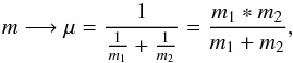 (A.2)and the relative velocity
 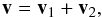 (A.3)by taking the square of the relative velocity and by doing the average we obtain
 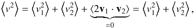 (A.4)where ⟨2v1·v2⟩ = 0 because of the isotropy of v2.
In the simplest case (m1 = m2 and all the particles are at Tgas) through the equation below 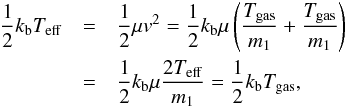 (A.5)it is possible to find the effective temperature of the molecules
  (A.6)In the case (our case) of two different molecules (i.e. CO and O, mCO ≠ mO) at different temperatures (TCO = Tsolid ≠ Tgas = TO or TO = Tsolid ≠ Tgas = TCO), we will have a reduced mass of
 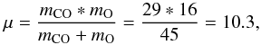 (A.7)then, in the case of CO adsorbed and O arriving from the gas phase,
 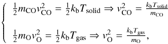 or, in the case of O adsorbed and CO from gas phase,
 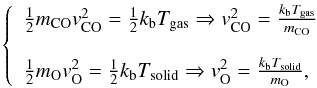 and so
 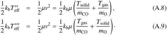 From these equations, by using Tsolid = 25 K and Tgas = 300, we obtain
 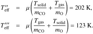 These two Teff will be used to find a lower and an upper limit for the activation barrier. We have to note that the two reactions Ogas + COsolid and COgas + Osolid do not have the same probability of occurring at different temperatures due to a different residence time on the surface and diffusion constant of molecules and atoms and, in the case of Osolid strong concurrence with O + O2 reaction. This consideration induces us not to give an exact value of the activation barrier, but just a possible range of values.
All Tables
Model results showing carbon dioxide yields as a function of surface temperature.
All Figures
|
Fig. 1 Schematic top-view of the FORMOLISM setup and the FT-RAIRS facility. |
| In the text | |
|
Fig. 2 TPD curves of mass 45 (13CO2) between 60 and 120 K after 4 ML of 13CO exposure (dotted curve), and after 4 ML of 13CO + O (solid line) on graphite held at 10 K. |
| In the text | |
|
Fig. 3 TPD curves of mass 45 (13CO2) between 65 and 125 K after deposition of 1 ML of 13CO (squares), 13CO + O2 (circles) and 13CO + O3 (triangles) on graphite held at 10 K. |
| In the text | |
|
Fig. 4 TPD curves at mass 29, 32, and 45 after irradiation of 0.5 ML of 13CO + O on ASW ice held at 20 K. Four peaks are visible. The first peak between 28 K and 42 K is due to O2 desorption, the second one between 32 and 55 K is due to 13CO desorption. The third peak between 55 K and 75 K represents O3 desorption, while the high-temperature peak is the desorption of 13CO2 (75−95 K). |
| In the text | |
|
Fig. 5 13CO2 yield as a function of surface temperature during deposition of 0.5 ML of 13CO + O. Circles represent the integrated area under the TPD curves of mass 45 after a deposition of 0.5 ML of 13CO + O on ASW ice held at different temperatures (10 K, 20 K, 30 K, 35 K, 40 K, 45 K, 50 K, 60 K). The solid line is a fit of the area behaviour. The TPD peaks (obtained at Tsurface = 20 K) added in the figure show when O2 and 13CO desorb, and this helps interpret the 13CO2 yield behaviour with temperature. |
| In the text | |
|
Fig. 6 O2 and O3 yields as a function of surface temperature during deposition of 0.5 ML of 13CO + O. The circles and the squares represent the integrated area under the TPD curves of O2 and O3, respectively, after deposition of 0.5 ML of 13CO + O on ASW ice held a different temperatures (10 K, 20 K, 30 K, 35 K, 40 K, 45 K, 50 K, 60 K). The solid line is a fit of the area behaviour. The added O2 TPD (obtained at Tsurface = 20 K) helps interpret the O3 yield behaviour with temperature. |
| In the text | |
|
Fig. 7 Model results for CO2 production on ASW (pure ER). The curves in this figure were obtained by using rLH = 0, and different rER values (ranging from 0.005 to 0.1). The squares are a best fit of the experimental values. |
| In the text | |
|
Fig. 8 Model results for CO2 production on ASW (pure LH). The curves in this figure were obtained by using rER = 0, and different rLH values (ranging from 0.001 to 0.02). The squares are a best fit of the experimental values. |
| In the text | |
|
Fig. 9 Model results for all species on ASW. The curves in this figure were obtained by using rLH = 0.0019 ± 0.0005 and rER = 0.021 ± 0.007. The circles, stars, triangles and squares represent O2, CO2, CO, and O3 experimental results respectively. The inset displays a magnified view of the CO2 yield around its maximum for clarity. |
| In the text | |
|
Fig. 10 Model results showing the contribution to CO2 formation by either ER (triangles) or LH (circles) mechanism. Contributions to CO2 formation are expressed in monolayers (ML) as a function of surface temperature. |
| In the text | |
|
Fig. 11 Temperature dependence of rLH(T) between 10 and 60 K. The two pinstriped regions indicate how a different parametrization of tunneling for CO + O reaction and of O2 and CO diffusion can change our estimation of rLH(T). The dashed line represents our experimental data. Full circles are an example of a pure Arrhenius behaviour. |
| In the text | |
Current usage metrics show cumulative count of Article Views (full-text article views including HTML views, PDF and ePub downloads, according to the available data) and Abstracts Views on Vision4Press platform.
Data correspond to usage on the plateform after 2015. The current usage metrics is available 48-96 hours after online publication and is updated daily on week days.
Initial download of the metrics may take a while.