| Issue |
A&A
Volume 559, November 2013
|
|
|---|---|---|
| Article Number | A102 | |
| Number of page(s) | 22 | |
| Section | Stellar atmospheres | |
| DOI | https://doi.org/10.1051/0004-6361/201321036 | |
| Published online | 21 November 2013 | |
Three-dimensional hydrodynamical CO5BOLD model atmospheres of red giant stars
III. Line formation in the atmospheres of giants located close to the base of the red giant branch⋆
1
Vilnius University Astronomical Observatory,
M. K. Čiurlionio 29,
03100
Vilnius,
Lithuania
e-mail:
Vidas.Dobrovolskas@ff.vu.lt
2
Vilnius University Institute of Theoretical Physics and Astronomy,
A. Goštauto 12,
01108
Vilnius,
Lithuania
e-mail: arunas.kucinskas@tfai.vu.lt;
jonas.klevas@tfai.vu.lt; dainius.prakapavicius@tfai.vu.lt
3
Leibniz-Institut für Astrophysik Potsdam,
An der Sternwarte
16, 14482
Potsdam,
Germany
e-mail: msteffen@aip.de
4
Landessternwarte – Zentrum für Astronomie der Universität
Heidelberg, Königstuhl
12, 69117
Heidelberg,
Germany
e-mail: hludwig@lsw.uni-heidelberg.de; elcaffau@lsw.uni-heidelberg.de
5
GEPI, Observatoire de Paris, CNRS, Université Paris Diderot,
Place Jules
Janssen, 92190
Meudon,
France
e-mail:
piercarlo.bonifacio@obspm.fr
Received:
3
January
2013
Accepted:
22
July
2013
Aims. We utilize state-of-the-art three-dimensional (3D) hydrodynamical and classical 1D stellar model atmospheres to study the influence of convection on the formation properties of various atomic and molecular spectral lines in the atmospheres of four red giant stars, located close to the base of the red giant branch, RGB (Teff ≈ 5000 K, log g = 2.5), and characterized by four different metallicities, [M/H] = 0.0, −1.0, −2.0, −3.0.
Methods. The role of convection in the spectral line formation is assessed with the aid of abundance corrections, i.e., the differences in abundances predicted for a given equivalent width of a particular spectral line with the 3D and 1D model atmospheres. The 3D hydrodynamical and classical 1D model atmospheres used in this study were calculated with the CO5BOLD and 1D LHD codes, respectively. Identical atmospheric parameters, chemical composition, equation of state, and opacities were used with both codes, therefore allowing a strictly differential analysis of the line formation properties in the 3D and 1D models.
Results. We find that for lines of certain neutral atoms, such as Mg i, Ti i, Fe i, and Ni i, the abundance corrections strongly depend both on the metallicity of a given model atmosphere and the line excitation potential, χ. While abundance corrections for all lines of both neutral and ionized elements tend to be small at solar metallicity (≤±0.1 dex), for lines of neutral elements with low ionization potential and low-to-intermediate χ they quickly increase with decreasing metallicity, reaching in their extremes −0.6 to −0.8 dex. In all such cases the large abundance corrections are due to horizontal temperature fluctuations in the 3D hydrodynamical models. Lines of neutral elements with higher ionization potentials (Eion ≳ 10 eV) generally behave very similarly to lines of ionized elements characterized by low ionization potentials (Eion ≲ 6 eV). In the latter case, the abundance corrections are small (generally, ≤±0.1 dex) and are caused by approximately equal contributions from the horizontal temperature fluctuations and differences between the temperature profiles in the 3D and 1D model atmospheres. Abundance corrections of molecular lines are very sensitive to the metallicity of the underlying model atmosphere and may be larger (in absolute value) than ~−0.5 dex at [M/H] = −3.0 (~−1.5 dex in the case of CO). At fixed metallicity and excitation potential, the abundance corrections show little variation within the wavelength range studied here, 400−1600 nm. We also find that an approximate treatment of scattering in the 3D model calculations (i.e., ignoring the scattering opacity in the outer, optically thin, atmosphere) leads to abundance corrections that are altered by less than ~0.1 dex, both for atomic and molecular (CO) lines, with respect to the model where scattering is treated as true absorption throughout the entire atmosphere, with the largest differences for the resonance and low-excitation lines.
Key words: stars: atmospheres / stars: late-type / stars: abundances / convection / hydrodynamics
Appendices and Figs. 3, 5, 6, 8, 9, 11 are available in electronic form at http://www.aanda.org
© ESO, 2013
1. Introduction
All low and intermediate mass stars evolve through the red giant stage. Owing to their large numbers, red giants are important tracers of intermediate-age and old stellar populations, and their high luminosities make them accessible for observations both in and beyond the Milky Way. This makes them particularly suitable for use in spectroscopic studies that aim to understand the chemical evolution of their host populations. On the other hand, stars on the red giant branch (RGB) experience mixing episodes during which material with the chemical composition altered via nuclear reactions is brought to the stellar surface. Elemental abundances in the atmospheres of red giant stars may therefore provide a wealth of important information about the nucleosynthesis and mixing processes in stars and about the chemical evolution histories of their host populations.
To obtain information from stellar spectra about the abundances of the chemical species of interest one has to rely on stellar model atmospheres. Inevitably, the confidence with which one can derive chemical composition of stars is determined by the accuracy and physical realism of the underlying model atmospheres. Classical 1D model atmospheres are most widely used for such tasks today. Stellar atmospheres in these models are treated as static and 1D, so that resulting model structures are functions of the radial coordinate alone. Convection in such models is described by using the mixing-length theory (MLT; see, e.g., Böhm-Vitense 1958; Canuto & Mazzitelli 1991), along with a number of free parameters, such as the mixing-length parameter, αMLT, and microturbulence velocity. Thanks to their static 1D nature and various simplifications involved, such models are fast to compute, which allowed large model grids to be produced using a variety of 1D model atmosphere codes, such as ATLAS (Castelli & Kurucz 2003), MARCS (Gustafsson et al. 2008), and PHOENIX (Brott & Hauschildt 2005), for various combinations of stellar atmosphere parameters. Despite numerous simplifications, 1D model atmospheres have aided in gaining enormous amounts of information about the processes taking place in stellar atmospheres and deeper interiors.
Since stellar atmospheres are neither static nor 1D, a large increase in computational power is required to include more realistic 3D time-dependent physics into stellar atmosphere modeling. Mostly because of such computational complexities the advance of 3D hydrodynamical model atmospheres and their applications in stellar abundance work has been relatively slow. Despite this, there has been a notable increase in the applications of the 3D hydrodynamical model atmospheres to study stars and stellar populations during the recent years (see, e.g., Asplund et al. 2000; Caffau et al. 2008; González Hernández et al. 2009; Behara et al. 2010). This is partly related to the fact that a number of studies have shown that differences in the elemental abundances inferred from the same spectral line strength with the classical 1D and 3D hydrodynamical model atmospheres may be significant, especially at lower metallicities where they may reach −1.0 dex (see, e.g., Collet et al. 2007; Dobrovolskas et al. 2010; Ivanauskas et al. 2010). Obviously, such differences in the obtained abundances may lead to important implications, such as when reconstructing most likely scenarios of chemical evolution of stellar populations in the Galaxy and beyond.
To take a closer look at the role of convection in the spectral line formation in the atmospheres of red giant stars, we started a systematic study of the internal structures and observable properties of red giant stars by using 3D hydrodynamical CO5BOLD model atmospheres for this purpose. In the first two papers in this series (Ludwig & Kučinskas 2012; Kučinskas et al. 2013, Papers I and II hereafter), we investigated the role of convection on the atmospheric structures and spectral line formation in a red giant star located close to the RGB tip (Teff ≈ 3660 K, log g = 1.0, [M/H] = 0.0). In this study we extend our previous work and focus on the properties of spectral line formation in somewhat warmer red giants at several different metallicities ([M/H] = 0.0, −1.0, −2.0, −3.0) located close to the RGB base (Teff ≈ 5000 K, log g = 2.5).
The paper is structured as follows. In Sect. 2 we describe the 3D hydrodynamical and classical 1D model atmospheres used in this study, and outline the details of spectral line synthesis calculations. In this section we also introduce the concept of abundance corrections, which is used throughout the paper to assess the differences in the abundances predicted for the same line strength with the 3D and 1D model atmospheres. The abundance corrections obtained for various neutral and ionized atoms and for molecules are discussed in Sect. 3, together with the role of scattering and the importance of the mixing-length parameter, αMLT, used with the 1D model atmospheres. Finally, summary and conclusions are provided in Sect. 4.
2. Stellar atmosphere models and spectral line synthesis calculations
In this study we utilized the CO5BOLD and LHD model atmosphere codes to calculate, respectively, the 3D hydrodynamical and classical 1D atmosphere models of red giants located close to the RGB base. Both CO5BOLD and LHD simulations shared identical atmospheric parameters, chemical composition, opacities, and equation of state, in order to limit the discrepancies in the model predictions to differences in the underlying model physics. Such differential comparison of the model predictions allows us to assess the importance of 3D hydrodynamical effects on the spectral line formation, and enables us to determine the differences between the abundances of different chemical elements derived with the 3D and 1D model atmospheres. In what follows below we briefly describe the details of model atmosphere and spectral line synthesis calculations.
2.1. 3D hydrodynamical CO5BOLD stellar model atmospheres
The 3D hydrodynamical models used in this study are part of the CIFIST model atmosphere grid which will eventually cover stars on the main sequence, subgiant, and red giant branches (Ludwig et al. 2009). CO5BOLD solves the coupled nonlinear equations of compressible hydrodynamics in an external gravity field, together with radiative transfer equation (Freytag et al. 2012). The model atmospheres were computed using the “box-in-a-star” setup, i.e., the part of the stellar atmosphere modeled was small compared to the size of a star itself. The simulations were performed on a Cartesian grid of 160 × 160 × 200 grid points in x,y,z directions, respectively. The model box had open upper and lower boundaries (matter was allowed to enter and leave the simulation box freely), and periodic boundaries in the horizontal direction (matter leaving the box on one side was allowed to enter it again from the opposite side). We used monochromatic opacities from the MARCS stellar atmosphere package (Gustafsson et al. 2008) which we grouped into a smaller number of opacity bins using the opacity binning technique (Nordlund 1982; Ludwig 1992; Ludwig et al. 1994; Vögler 2004; Vögler et al. 2004), with five opacity bins for the [M/H] = 0.0 model and six bins for the [M/H] = −1.0, −2.0, and −3.0 models. Solar-scaled elemental abundances used were those from Asplund et al. (2005). It is important to stress that we also applied a constant enhancement in the alpha-element abundances of [α/Fe] = +0.4 for the models at metallicities [M/H] ≤ −1.0. All model simulations were performed under the assumption of local thermodynamic equilibrium, LTE. Scattering was treated as true absorption and magnetic fields were neglected.
Parameters of the CO5BOLD red giant models used in this work.
Parameters of the individual 3D model atmospheres used in this work are provided in Table 1. One may notice that each model is characterized by a slightly different average effective temperature, ⟨Teff⟩. This is because effective temperature is not the input parameter for calculating 3D model atmosphere with the CO5BOLD code. Instead, one sets the value of entropy of inflowing gas at the bottom of the model atmosphere. This determines radiative flux at the outer boundary and thus − the effective temperature of a given model. Another important aspect is that radiative flux leaving the model atmosphere is subject to random spatial and temporal fluctuations due to stochastic nature of convection, which causes the effective temperature to fluctuate too. Therefore, the effective temperature of the 3D hydrodynamical model atmosphere can not be set in advance and should be fine-tuned by adjusting the entropy inflow at the lower boundary of the model atmosphere. Note, however, that differences between the average Teff of individual 3D model atmospheres are small (<30 K) while the effective temperatures of all models are very close to the target value of Teff = 5000 K (Table 1).
Since 3D spectral line synthesis calculations are very computationally demanding, we selected a smaller subset of 3D atmospheric structures at different instants of time (snapshots) to be used in all 3D line synthesis work. At all metallicities, these subsets consisted of 20 snapshots spaced with a step of ~7 h over the interval of ~4.7−6.5 days in stellar time. Since the convective time scales in the red giant models studied here are equal to ~5−15 h (as measured by the Brunt-Vaisälä time scale), such spacing of the 3D snapshots allows to consider them statistically independent. Snapshots of the 3D model were selected so that statistical properties of the 20-snapshot ensemble would best reproduce the corresponding properties of the entire model run, such as the average effective temperature and its standard deviation, mean velocity at optical depth unity, mean velocity profile and mean mass velocity profile.
In this study we also used average ⟨3D⟩ models. At each metallicity, these model atmospheres were computed by horizontally averaging each 3D atmospheric structure in the subset of twenty 3D model snapshots selected for the line synthesis calculations, as described above (the fourth power of temperature was averaged on surfaces of equal optical depth). The fourth power of temperature was chosen over the first because in the former case one may expect to retain better representation of the radiative flux throughout the model atmosphere. On the other hand, we found that differences in the ⟨3D⟩ abundances obtained with the models computed by averaging the fourth and first powers of temperature were always small (for example, in case of Fe i and Fe ii lines with χ = 0−6 eV these differences were typically significantly below 0.05 dex). We refer the reader to Appendix A where we provide some further thoughts regarding the choice of temperature averaging scheme. Every ⟨3D⟩ model is a 1D structure, hence the average ⟨3D⟩ models do not contain information about the horizontal fluctuations of thermodynamic quantities and velocity fields. Therefore, they can be used to estimate the role of horizontal fluctuations on, e.g., the spectral line formation, which can be done by comparing the predictions of the 3D and ⟨3D⟩ models.
2.2. 1D LHD model atmospheres
1D models were calculated using the LHD code (see, e.g., Caffau et al. 2008). We recall that both 3D and 1D models used in this work shared identical atmospheric parameters (Table 1), chemical composition, equation of state, and opacities (see Sect. 2.1 for details). Convection in the LHD models was treated according to the formalism of the mixing-length theory by Mihalas (1978). The mixing-length parameter used throughout the LHD simulations was αMLT = 1.0. In principle, the use of 1D models calculated with different mixing-length parameters results in different abundance corrections. However, in the case of the giants studied here it is only relevant for high-excitation atomic lines (see Sect. 3.5). Temperature stratifications of the 3D and 1D models at [M/H] = 0.0 and −3.0 are shown in Figs. 1 and 2, respectively.
2.3. Spectral line synthesis
In order to investigate the influence of convection on the spectral line formation we utilized fictitious spectral lines. For these lines, their central wavelengths, excitation potentials, χ, and oscillator strengths, log gf, were freely chosen to cover the range of values of existing spectral lines. Such approach allows us to study the connections between the atomic line parameters and line formation properties in the presence of realistically modeled convection, and has been already applied successfully in a number of studies (e.g., Steffen & Holweger 2003; Collet et al. 2007; Dobrovolskas et al. 2010; Ivanauskas et al. 2010; Paper II).
In this study, equivalent widths of synthetic spectral lines were fixed to W ≤ 0.5 pm. Because these lines are very weak, they should be confined to the linear part of the curve of growth and thus their strengths should be independent of the choice of microturbulence velocity, ξmic, used in the spectral line synthesis with the ⟨3D⟩ and 1D model atmospheres. In such situation, the differences in the line strengths predicted by the 3D and 1D model atmospheres can be attributed to purely 3D hydrodynamical effects, allowing investigation of their importance in the spectral line formation.
Spectral line synthesis calculations for all chemical elements studied in this work were done using the Linfor3D1 code, which solves the radiative transfer equation under the assumption of LTE. In order to speed up spectral line synthesis calculations, we used only every third point of the original 3D model structure along the x and y spatial directions. We verified that such simplification has left the resulting elemental abundances essentially unchanged (i.e., with respect to the calculations performed using the full model box). The differences were always below 0.003 dex in the case of [M/H] = −3 metallicity model and Fe i lines. In our simulations the radiative transfer was solved for 3 vertical and 4 azimuthal directions. Line synthesis calculations covered the Rosseland optical depth range from log τRoss = −6 to 2, in steps of Δlog τRoss = 0.08. Line profiles were computed with a typical wavelength resolution of 130−150 points per profile. In case of the 3D model atmospheres, spectral line profiles of every chemical element studied here were calculated for each of the twenty 3D model snapshots, at each of the four metallicities. The obtained individual spectral line profiles were then co-added to obtain the final 3D line profile at each metallicity. Similarly, in case of the average 3D models line profiles were calculated for every horizontally averaged 3D model structure from the 20-snapshot ensemble; the final ⟨3D⟩ line profile was then obtained by co-adding all twenty individual line profiles. All 1D line profiles were also calculated using the Linfor3D code. A microturbulence velocity of ξmic = 1.0 km s-1 was used in all ⟨3D⟩ and 1D spectral synthesis calculations, although we note again that the choice of ξmic does not change the line strength of very weak fictitious lines studied here.
One may envision that, alternatively, all 3D model snapshots could be averaged to produce a single ⟨3D⟩ model for the synthesis of ⟨3D⟩ spectral lines, i.e., instead of using individual averaged 3D models for each 3D snapshot as we did in this study. Our test calculations showed, however, that in case of Fe i and Fe ii lines with χ = 0−6 eV differences in the line profiles computed using these two different approaches would lead to differences in the elemental abundances of less than 0.03 dex (in case of Fe i lines they were always smaller than 0.01 dex). Therefore, for the purposes of present study the choice in the procedure used to compute the ⟨3D⟩ line profiles is of minor importance.
2.4. 3D–1D abundance corrections
The role of 3D hydrodynamical effects in spectral line formation was studied by utilizing 3D–1D abundance corrections. The 3D–1D abundance correction, Δ3D−1D, is the difference in the abundance, A(Xi), of a chemical element Xi obtained at a given equivalent width from the 3D and 1D curves of growth, Δ3D−1D ≡ A(Xi)3D − A(Xi)1D (see, e.g., Caffau et al. 2011). The 3D–1D abundance correction is sensitive to the effects related to both the horizontal temperature fluctuations and differences in temperature stratifications of the 3D and 1D model atmospheres. The size of these effects can be measured separately, by utilizing information content of the ⟨3D⟩ models. Since the ⟨3D⟩ model does not contain information about the horizontal fluctuations of thermodynamic quantities and velocity fields, the Δ3D−⟨ 3D ⟩ ≡ A(Xi)3D − A(Xi)⟨ 3D ⟩ correction can be used to measure the effect of horizontal temperature fluctuations. Similarly, the Δ⟨ 3D ⟩ −1D ≡ A(Xi)⟨ 3D ⟩ − A(Xi)1D correction provides information about the role of differences between the temperature profiles of the average ⟨3D⟩ and 1D models. Obviously, the final abundance correction is a sum of the two constituents, Δ3D−1D ≡ Δ3D−⟨ 3D ⟩ +Δ⟨ 3D ⟩ −1D.
3D–1D abundance corrections were calculated for a number of neutral and singly ionized elements: Li i, C i, O i, Na i, Mg i, Al i, Si i, Si ii, K i, Ca i, Ca ii, Ti i, Ti ii, Fe i, Fe ii, Ni i, Zn i, Zr i, Zr ii, Ba ii, and Eu ii. These elements allow to sample different nucleosynthetic channels: proton capture (Na, Al, K), triple-α (carbon), α-chain captures (O, Mg, Si, Ca, Ti), nuclear statistical equilibrium (Ti, Fe, Ni, Zn), slow neutron capture (Zn, Zr, Ba), rapid neutron capture (Ba, Eu). Lithium is a special element in this context, in a sense that it was produced during the Big-Bang nucleosynthesis and by several other processes afterwards, including cosmic ray spallation in the interstellar medium and several stellar processes. We also obtained abundance corrections for several molecules: CH, CO, C2, NH, CN, and OH which are important tracers of CNO elements.
The 3D–1D abundance corrections for neutral and ionized atoms were calculated at three wavelengths, λ = 400, 850 and 1600 nm. The two shorter wavelengths were chosen to bracket the typical blue and red limits of modern optical spectrographs, such as UVES/GIRAFFE@VLT, HIRES@Keck, HDS@SUBARU, while the longer approximately coincides with the H-band of near-infrared spectrographs, such as CRIRES@VLT, NIRSPEC@Keck. The two longest wavelengths also coincide with the maximum and minimum absorption of the H− ion at ~850 and ~1640 nm, respectively, while the bluest marks the spectral region where H− absorption becomes progressively smaller and opacities from various metals become increasingly more important. In case of the molecules, we used the wavelengths of real molecular lines/bands in the blue part of the spectrum (see Paper II for detailed description of the wavelength selection). In case when real molecular bands were not available at these short wavelengths, abundance corrections were obtained at λ = 400 nm instead. The abundance corrections were computed at four excitation potentials, χ = 0, 2, 4, and 6 eV, for both neutral and ionized atoms, while for the molecules they were obtained at χ = 0, 1, 2, and 3 eV.
Finally, we note that some species studied here have either only a few observable spectral lines or their lines may be simply too weak to be detected (as it is the case with, e.g., Li i, C i, O i). We should stress that such elements were included in the present analysis because we aimed to understand the general properties of spectral line formation in the presence of convection, especially the trends of abundance corrections in a wider range of atomic line parameters. Obviously, in all such cases the exact values of abundance corrections in a wide atomic parameter range may only be of academic interest.
3. Results and discussion
3.1. Abundance corrections for lines of neutral atoms
The 3D–1D abundance corrections for neutral atoms are plotted in Figs. 3−5 for λ = 400, 850, and 1600 nm, respectively. Each figure shows three abundance corrections, Δ3D−⟨ 3D ⟩, Δ⟨ 3D ⟩ −1D, and Δ3D−1D, plotted versus metallicity at four different line excitation potentials, χ = 0, 2, 4, and 6 eV.
For some elements, one may notice a strong dependence of the abundance corrections on
metallicity: corrections are small at [M/H] = 0.0 and −1.0 but they
grow quickly with decreasing metallicity and for certain elements may reach up to
−0.8 dex at [M/H] = −3.0 (Figs. 3–5). Abundance corrections are largest at
the lowest excitation potentials, χ = 0,2 eV, but they
quickly decrease with increasing χ: corrections then become both small
(less than ±0.1 dex) and essentially independent of metallicity. Such behavior is defined
by the atomic properties of chemical elements and the location of line formation regions
associated with particular spectral lines. At all metallicities, lines with lower
excitation potentials form in the outer atmospheric layers, but their formation regions
shift deeper into the atmosphere with increasing χ (Figs. 1−2). At solar
metallicity, differences between the temperature profiles of the ⟨3D⟩ and 1D model
atmospheres are small and change very little throughout the entire model atmosphere.
Similarly, horizontal temperature fluctuations, as measured by their rms value
( ,
here the angle brackets denote temporal and horizontal averaging on surfaces of equal
optical depth, and
T0 = ⟨ T ⟩ x,y,t,
is the depth-dependent average temperature) are not large either (i.e., compared with
their extent at lower metallicities) and change little with optical depth (Fig. 1). Therefore, at solar metallicity all three abundance
corrections, Δ3D−⟨ 3D ⟩, Δ⟨ 3D ⟩ −1D, and Δ3D−1D,
are small and nearly independent of the line excitation potential. On the other hand,
differences in the temperature profiles of the ⟨3D⟩ and 1D models are larger in the outer
atmosphere of low metallicity models (Fig. 2).
Horizontal temperature fluctuations are also largest in the outer atmosphere, besides,
they increase rapidly with decreasing metallicity. Consequently, at
[M/H] < −1.0 the abundance corrections
for most elements are largest for low-excitation lines, i.e., those that form farthest in
the atmosphere. For such lines, Δ3D−⟨ 3D ⟩ correction is significantly
larger than Δ⟨ 3D ⟩ −1D, especially at lowest metallicities. Also, the two
abundance corrections are nearly always of opposite sign, thus the absolute value of the
total correction, | Δ3D−1D |, is smaller than the sum
| Δ3D−⟨ 3D ⟩| + |Δ⟨ 3D ⟩ −1D |.
,
here the angle brackets denote temporal and horizontal averaging on surfaces of equal
optical depth, and
T0 = ⟨ T ⟩ x,y,t,
is the depth-dependent average temperature) are not large either (i.e., compared with
their extent at lower metallicities) and change little with optical depth (Fig. 1). Therefore, at solar metallicity all three abundance
corrections, Δ3D−⟨ 3D ⟩, Δ⟨ 3D ⟩ −1D, and Δ3D−1D,
are small and nearly independent of the line excitation potential. On the other hand,
differences in the temperature profiles of the ⟨3D⟩ and 1D models are larger in the outer
atmosphere of low metallicity models (Fig. 2).
Horizontal temperature fluctuations are also largest in the outer atmosphere, besides,
they increase rapidly with decreasing metallicity. Consequently, at
[M/H] < −1.0 the abundance corrections
for most elements are largest for low-excitation lines, i.e., those that form farthest in
the atmosphere. For such lines, Δ3D−⟨ 3D ⟩ correction is significantly
larger than Δ⟨ 3D ⟩ −1D, especially at lowest metallicities. Also, the two
abundance corrections are nearly always of opposite sign, thus the absolute value of the
total correction, | Δ3D−1D |, is smaller than the sum
| Δ3D−⟨ 3D ⟩| + |Δ⟨ 3D ⟩ −1D |.
 |
Fig. 1 Upper panel: temperature profiles in the red giant model with Teff/log g/ [M/H] = 4970/2.5/0.0, plotted versus the Rosseland optical depth, τRoss, and shown for the following model atmospheres: 3D (density plot), ⟨3D⟩ (dashed line), and 1D (solid line). Horizontal bars mark the approximate location of the Fe I and Fe II line formation regions in the 3D (black) and 1D (blue) atmosphere models, at λ = 400 nm and χ = 0 and 6 eV (bars mark the regions where the equivalent width, W, of a given spectral line grows from 5% to 95% of its final value). Lower panel: rms horizontal temperature fluctuations in the 3D model (solid line), and difference between the temperature profiles of the ⟨3D⟩ and 1D models (dashed line), shown as functions of the Rosseland optical depth. In both panels, all quantities related to the 3D and ⟨3D⟩ models were obtained using the subset of twenty 3D model snapshots utilized in the 3D spectral line synthesis calculations (see Sect. 2.1). |
 |
Fig. 4 Abundance corrections for spectral lines of neutral atoms plotted versus metallicity at λ = 850 nm: Δ3D−⟨ 3D ⟩ (left column), Δ⟨ 3D ⟩ −1D (middle column), and Δ3D−1D (right column). Corrections are given at several different excitation potentials, as indicated on the right side of each row. Abundance corrections at λ = 400 nm and λ = 1600 nm (Figs. 3 and 5, respectively) are available in the online version only. |
 |
Fig. 7 Same as in Fig. 3 but for lines of ionized atoms, plotted versus metallicity and excitation potential at λ = 850 nm. Abundance corrections at λ = 400 nm and λ = 1600 nm (Figs. 6 and 8, respectively) are available in the online version only. |
One may notice however, that the size of Δ3D−1D corrections at a given low metallicity may be very different for different elements, ranging roughly from −0.8 dex to +0.1 dex at [M/H] = −3.0 (Figs. 3–5). Such differences are caused by the interplay of ionization and excitation. Elements with small ionization potential (such as Li i, Na i, K i) are nearly completely ionized throughout the entire atmosphere, at all metallicities. Therefore, neutral atoms of such elements are in their minority ionization stage. In all such cases the line opacity, κℓ, can be roughly approximated as κℓ ~ 10θ (Eion − χ), where θ = 5040/T and Eion is the ionization energy of a given element (see Paper II, Appendix A, Eq. (A.5)). In such cases, the line opacity becomes a very sensitive function of the temperature at low χ. Consequently, for lines with low χ large temperature fluctuations in the outer atmospheric layers at low metallicities cause large variations in the line strength, which translate into large abundance corrections Δ3D−⟨ 3D ⟩, and thus Δ3D−1D. On the other hand, neutral elements with high Eion, such as C i, O i, are in their majority ionization stage. In such case, the excitation potential dominates over the ionization energy and thus the high-excitation lines become most sensitive to the temperature variations. In fact, the dependence of all abundance corrections for C i and O i on both [M/H] and χ is very similar to those of ionized elements.
Abundance corrections in the infrared wavelength range are very similar to those obtained either at λ = 400 or 850 nm and for certain elements may reach up to Δ3D−1D = −0.7 dex. This is in contrast to the results obtained by us for significantly cooler red giant at Teff = 3600 K, log g = 1.0, and [M/H] = 0.0 for which the abundance corrections at 1600 nm were significantly smaller than those in the optical wavelength range (Paper II). Obviously, the latter does not hold for the red giants studied here since their abundance corrections are large at all wavelengths (see Appendix B for a detailed discussion). These results therefore suggest that the use of 3D hydrodynamical models may in fact be necessary for the abundance diagnostics with lines of neutral atoms in red giants at low metallicities.
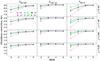 |
Fig. 10 Same as in Fig. 3 but for molecular lines plotted versus metallicity and excitation potential at λ = 850 nm. Abundance corrections at λ = 400 nm and λ = 1600 nm (Figs. 9 and 11, respectively) are available in the online version only. |
3.2. Abundance corrections for lines of ionized atoms
The 3D–1D abundance corrections for ionized atoms are shown in Figs. 6−8, at λ = 400, 850, and 1600 nm, respectively. As in the case with neutral atoms, we provide three abundance corrections, Δ3D−⟨ 3D ⟩, Δ⟨ 3D ⟩ −1D, and Δ3D−1D, plotted versus metallicity at four different line excitation potentials, χ = 0, 2, 4, and 6 eV.
At all [M/H] and χ studied here, the abundance corrections for lines of ionized atoms are confined to the range of ~±0.1 dex and show little sensitivity to changes in both metallicity and excitation potential (i.e., if compared to trends seen with lines of neutral atoms). Lines of ionized atoms form significantly deeper in the atmosphere where both the horizontal temperature fluctuations (which determine the size of Δ3D−⟨ 3D ⟩ correction) and the differences between temperature profiles of the ⟨3D⟩ and 1D models (which influence the size of Δ⟨ 3D ⟩ −1D correction) are smallest at all metallicities and change little with [M/H]. This leads to small abundance corrections that are insensitive to changes in [M/H] and χ. On the other hand, elements with lower ionization energies (Eion < 6 eV) are nearly completely ionized throughout the entire atmosphere of red giants studied here. For lines of such ionized elements it is the excitation potential that determines the line opacity, κℓ, and thus the strengths of high-excitation lines are most sensitive to temperature fluctuations (see Paper II, Appendix B). Since temperature fluctuations are in fact smallest at the depths where such lines form, and because this holds at all metallicities, this too leads to Δ3D−1D corrections that are small and show little variation with either metallicity or excitation potential (though, as expected, they increase slightly with χ).
It is worthwhile noting that Δ3D−⟨ 3D ⟩ and Δ⟨ 3D ⟩ −1D corrections are often of opposite sign, especially at the lowest metallicities, thus their sum leads to somewhat smaller total abundance corrections, Δ3D−1D. Since κℓ is a highly nonlinear function of temperature, horizontal temperature fluctuations produce larger line opacities leading to stronger lines and thus, negative Δ3D−⟨ 3D ⟩ corrections. On the other hand, since the temperature of the ⟨3D⟩ model is generally lower than that of the 1D model in the line forming regions, lines of ionized species are weaker in ⟨3D⟩ than in 1D. This leads to positive Δ⟨ 3D ⟩ −1D corrections. As in the case of neutral atoms, abundance corrections at λ = 1600 nm are comparable to those obtained at 400 and 850 nm and may reach to −0.1 dex at [M/H] = −3.0.
Qualitatively, the dependence of abundance corrections on metallicity and excitation potential seen in Figs. 3–7 for neutral and ionized atoms is very similar to the trends found by Collet et al. (2007), who computed abundance corrections for red giants with atmospheric parameters nearly identical to those used in our study. One obvious difference between the results obtained in the two studies is that our abundance corrections are somewhat smaller. It is possible, however, that this discrepancy may be traced back to differences between the underlying 3D model atmospheres, i.e., the STAGGER code used by Collet et al. (2007) and the CO5BOLD code utilized in our study. Indeed, the two codes use different opacities and opacity binning techniques, different equations of state, and so forth. One should also note a major difference in the 1D model atmospheres used as reference. While LHD models use the same opacities, microphysics, and numerical schemes used by CO5BOLD, the MARCS1˜D model atmosphere used as reference by Collet et al. (2007) uses opacities and EOS different from those used in their 3D model.
3.3. Abundance corrections for molecular lines
The 3D–1D abundance corrections for molecular lines are shown in Figs. 9, 10, and 11, at the bluest wavelength, 850 nm, and 1600 nm, respectively. We provide three abundance corrections, Δ3D−⟨ 3D ⟩, Δ⟨ 3D ⟩ −1D, and Δ3D−1D, plotted versus metallicity at four different excitation potentials, χ = 0, 1, 2, and 3 eV.
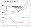 |
Fig. 12 Top panel: temperature profiles of the average ⟨3D⟩ model (Teff = 5020 K, log g = 2.5, and [M/H] = −3.0) calculated with scattering treated as true absorption (red solid line) and with scattering opacity neglected at small τRoss (red dashed line). Black lines mark the 5th and 95th percentiles of the temperature distribution in the 3D model with scattering treated as true absorption (solid lines) and scattering opacity neglected in optically thin regions (dashed lines). Horizontal bars indicate the approximate location where lines of several trace elements form at λ = 400 nm and χ = 0 and 4 eV and of the CO molecule at λ = 400 nm and χ = 0 and 3 eV (bars mark the regions where the equivalent width, W, of a given spectral line grows from 5% to 95% of its final value). Bottom panel: difference in the temperature profiles corresponding to the average ⟨3D⟩ models calculated with the two different treatments of scattering. |
As in the case of abundance corrections for neutral atoms, corrections for the molecules are strongly dependent on metallicity and are largest at the lowest metallicities. While for the majority of molecules the total abundance correction, Δ3D−1D, generally does not exceed −1.0 dex at [M/H] = −3.0, in the case of CO it reaches −1.5 dex. The large total abundance corrections are mostly due to the large Δ3D−⟨ 3D ⟩ corrections, which, as in the case of neutral and ionized atoms, indicates the importance of horizontal temperature fluctuations in the formation of molecular lines. The contribution due to differences in the average 3D and 1D temperature profiles, however, is also non-negligible, somewhat in contrast to the much less important Δ⟨ 3D ⟩ −1D abundance corrections in the case of neutral and ionized atoms.
The trends in the abundance corrections for molecules seen in Figs. 9−11 are determined by a subtle interplay of a number of different factors (see Appendix C for a more extended discussion). To briefly summarize, as in the case of the cool red giant studied in Paper II CO is the most abundant molecule in the atmospheric layers just above the optical surface (Fig. C.1). Since most of the carbon is locked into CO in the cooler regions (T ≤ 4000 K), only minor amounts of C are available to form other carbon-bearing molecules. In fact, this makes their number densities a highly nonlinear function of the local temperature. Since the line opacity is directly proportional to the number density of a given molecule, large horizontal temperature fluctuations (especially in the lowest metallicity models) should potentially lead to substantial abundance corrections.
In the following, we focus on the lowest metallicity model, [M/H] = −3.0, where the amplitude of the horizontal temperature fluctuations in the line forming regions is high and produces large variations of the molecular number densities. Therefore, the most pronounced molecular abundance corrections Δ3D−⟨ 3D ⟩ are derived for [M/H] = −3.0, χ = 0.0 eV (upper left panel of Fig. 9). We note that the magnitude of the correction is not simply a monotonic function of the dissociation energy of the molecule, D0. A monotonic increase of | Δ3D−⟨ 3D ⟩ | with D0 would be expected if all molecules were just minority species (see Eq. (C.1), Appendix C; and Eqs. (C.4), (C.5) in Paper II). In the atmosphere under investigation here, however, the temperature dependence of the number densities of the carbon-bearing molecules is influenced by the strong coupling with the formation of CO. In the hotter parts of the atmosphere, a temperature increase always leads to a destruction of the molecules, while in the cooler regions, where atomic carbon is a minority species, temperature increase leads to the destruction of CO, and in turn, to a larger concentration of atomic carbon that enables an enhanced formation of carbon-bearing molecules, which thus exhibit a reversed temperature sensitivity.
Such subtle interplay leads to the situation where it is difficult to predict the magnitude of the 3D corrections from the basic molecular properties. Here we rather interpret the numerical results provided by the spectrum synthesis calculations.
As is evident from Fig. C.3 (upper left panel), the number density of CO at any given optical depth in the atmosphere experiences the broadest range of fluctuations in the 3D model ([M/H] = −3.0). This is due to the fact that CO has the highest dissociation energy, D0 = 11.1 eV. Moreover, CO forms rather high in the atmosphere (Fig. C.2) where the largest horizontal temperature fluctuations are encountered. Consequently, the line opacity of CO experiences the largest variations in the line forming region, such that the average line opacity, ⟨ κℓ(T) ⟩ is significantly larger than the line opacity corresponding to the average temperature κℓ(⟨ T ⟩), leading to the largest (most negative) abundance corrections.
CH (D0 = 3.5 eV) and C2 (D0 = 6.3 eV) show the smallest (least negative) 3D corrections. Unexpectedly, the corrections for these two molecules are almost identical, although their dissociation energies are rather different. The explanation for this unexpected behavior is related to the fact that the temperature dependence of the line opacity at constant optical depth τRoss = −2 changes sign, both for CH and C2 (see middle panels of Fig. C.3 in Appendix C). In the high-temperature part (θ < 1.3), the slope ∂log κℓ/∂θ is more positive for C2 than for CH, in accordance with the different values of D0. But in the low-temperature regions (θ > 1.3), the slope is more negative for C2 than for CH, because X(C2) depends on X2(C), while X(CH) depends only linearly on X(C). This compensatory effect apparently leads to very similar effective amplification factors (see Appendix B) Aℓ = ⟨ κℓ(T) ⟩ /κℓ(⟨ T ⟩) for both molecules, and hence to similar abundance corrections.
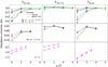 |
Fig. 13 Abundance corrections obtained for selected elements and for the CO molecule with the model atmospheres computed using different treatments of scattering (plotted versus the excitation potential χ, for lines at λ = 400 nm). For each element, two cases are shown: (a) with scattering treated as true absorption (solid lines), and (b) with scattering opacity neglected in the optically thin regions (dashed lines). Atmospheric parameters of the model atmospheres are Teff = 5020, log g = 2.5, and [M/H] = −3.0. Three types of abundance corrections are shown: Δ3D−⟨ 3D ⟩ (left column), Δ⟨ 3D ⟩ −1D (middle column), and Δ3D−1D (right column). |
The other molecules, CN (D0 = 7.8 eV), NH (D0 = 3.5 eV) and OH (D0 = 4.4 eV) occupy an intermediate position in the range of abundance corrections. NH and OH have similar molecular properties and line formation regions, and hence their corrections are similar, too. However, it is surprising that the corrections for NH and OH fall in the same range as those for CN, which has a much higher dissociation energy. Again, the explanation is related to the change of sign of the slope ∂log κℓ/∂θ in the case of CN, due to the coupling with CO at low temperatures, which is missing in the case of NH and OH, where the slope is therefore essentially constant over the whole temperature range (see Fig. C.3, lower panels).
These results qualitatively agree with those obtained by Collet et al. (2007), in a sense that the magnitude of abundance corrections for the molecules increases significantly with decreasing metallicity. However, quantitatively the results are different: abundance corrections at the lowest metallicity probed in our study ([M/H] = −3.0) are on average by 0.5−0.6 dex smaller compared with the corrections derived by Collet et al. (2007) using a model with similar atmospheric parameters. For example, for NH molecular line at λ = 336 nm and χ = 0 eV excitation potential we obtain Δ3D−1D ≈ −0.5 dex while Collet et al. (2007) gets Δ3D−1D ≈ −1.0 dex. Apparently, these discrepancies are due to differences in the temperature structure of the 3D models used in the two studies. Indeed, in the case of the Stein & Nordlund (1998) models used by Collet et al. (2007) the difference between the average ⟨3D⟩ and 1D temperature stratifications may reach ~1000 K at log τRoss ≈ −4 for the [M/H] = −3.0 model, whereas in our case these differences do not exceed ~300 K at log τRoss < −1 (Fig 2). We would like to stress once more that Collet et al. (2007) compare their 3D results with those obtained using 1D MARCS models; clearly, such approach is less self-consistent since differences in, e.g., equation of state, opacities used with the two model atmospheres may affect the resulting 3D–1D abundance corrections. The reason for the different temperature structures is presently not well understood but some possible reasons are discussed below.
3.4. Scattering and spectral line formation
The CO5BOLD models treat scattering as true absorption which may be seen as rather crude approximation. Indeed, as it was discussed recently by Collet et al. (2011), the treatment of scattering may have a significant impact on the thermal structure of 3D model atmospheres. In their study, coherent isotropic scattering was implemented in the model atmosphere code and the obtained model structures were compared with those where continuum scattering was treated either as true absorption or scattering opacity neglected in the optically thin regions. These tests have shown that in the former case the resulting temperature profiles were significantly warmer with respect to those calculated with coherent isotropic scattering. It has been thus argued by Collet et al. (2011) that the different thermal structures obtained with the STAGGER and CO5BOLD codes may be due to the different treatment of scattering. Interestingly, the authors also found that in case when scattering opacity was neglected in the optically thin regions the resulting temperature profile was very similar to that obtained when scattering was properly included into the radiative transfer calculations.
The role of scattering in the CO5BOLD model atmospheres has been recently studied by Ludwig & Steffen (2012) who compared thermal structures of the standard CO5BOLD models (i.e., those calculated with continuum scattering treated as true absorption) and the CO5BOLD models computed with continuum scattering opacity left out in the optically thin regions. Surprisingly, temperature profiles in the two models were different by only ~120 K at τRoss = −4.0, in contrast to ~600 K obtained by Collet et al. (2011). While the exact cause of this difference is still unclear, Ludwig & Steffen (2012) have suggested that they may be due to different procedures used to compute binned opacities used with the two types of models.
Obviously, it is important to understand the consequences that the differences in the treatment of scattering may have on the temperature stratification in the model atmosphere which, in turn, may influence the spectral line formation. We therefore calculated a number of fictitious lines of several chemical elements (Li i, O i, Na i, Fe i, Fe ii, Ni i, and Ba ii), by utilizing the CO5BOLD model in which scattering opacity was neglected in the optically thin regions (taken from Ludwig & Steffen 2012). According to the reasoning provided in Collet et al. (2011), the thermal structure of such models should be very similar to that in the models calculated with an exact treatment of scattering. Therefore, the comparison of line formation properties in these and standard models (i.e., those in which scattering is treated as true absorption) may allow to assess the importance of indirect effects of scattering on the spectral line formation via its influence on the temperature profiles. Since scattering becomes increasingly more important at low [M/H] where both line and continuum opacities are significantly reduced, the lowest metallicity CO5BOLD model was used for these tests (Teff = 5020 K, log g = 2.5, and [M/H] = −3.0). Spectral line synthesis was performed using 20 fully relaxed 3D snapshots of this test model, using the procedure identical to that utilized with the standard CO5BOLD models (see Sect. 2.3). The abundance corrections obtained with this and the standard model are shown in Fig. 13.
The obtained results suggest that differences in the treatment of scattering within the CO5BOLD setup have only minor influence on the spectral line strengths. The abundance corrections obtained for the standard CO5BOLD model and the one in which scattering opacity was neglected in the optically thin regions differ by less than 0.1 dex, both for neutral atoms and ions (see Fig. 13). For models with scattering opacity neglected, slightly lower temperature in the outer atmospheric layers (Fig. 12) leads to somewhat larger abundance corrections for the low-excitation spectral lines of neutral atoms (~0.1 dex). Since higher excitation lines form deeper in the atmosphere where differences in the thermal profiles are smaller, the influence of differences in the treatment of scattering becomes negligible for such lines, with changes in the abundance corrections of less than 0.01 dex at χ > 4 eV. Lines of ionized elements form deep in the atmosphere too, thus, irrespective of their excitation potential, differences in the treatment of scattering do not affect their line strengths.
The situation may be slightly different in case of molecular lines. The formation of such lines extends into the outer atmosphere where the differences in the treatment of scattering may have an impact on the resulting line strengths. Indeed, in case of CO the differences in the abundance corrections components Δ3D−⟨ 3D ⟩ and Δ⟨ 3D ⟩ −1D calculated using the two treatments of scattering may reach ~−0.2 dex and ~0.3 dex, respectively (Fig. 13). However, due to their opposite sign the full 3D−1D abundance correction Δ3D−1D becomes smaller, ~0.1 dex. Nevertheless, such differences may still be important in stellar abundance work.
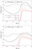 |
Fig. 14 Velocity profiles of the LHD models (red/gray lines) at [M/H] = 0.0 (top panel) and [M/H] = −3.0 (bottom panel) computed using three different mixing-length parameters, αMLT = 1,1.5,2.0. Vertical and horizontal velocity profiles of the average ⟨3D⟩ model (computed on the log τRoss iso-surfaces are shown as solid and dot-dashed black lines, respectively. |
Our results therefore suggest that the treatment of scattering may be important in case of the low-excitation lines with χ ≤ 2 eV and molecular lines. For elements such as sodium, where frequently only resonance or low-excitation lines are available for the abundance diagnostics, different recipes in the treatment of scattering may lead to systematic abundance differences of up to 0.1 dex at [M/H] = −3.0. On the other hand, strengths of high-excitation spectral lines, as well as lines of ionized elements, seem to be little affected by the choice of scattering prescription.
3.5. Influence of the mixing-length parameter αMLT on the abundance corrections
According to the Schwarzschild criterion for the onset of convection, LHD models predict that at Solar metallicity convective flux should be zero at around and above the optical depth unity (Fig. 14, top panel). The situation is slightly different at [M/H] = −3.0 where, because of the lower opacity, convection in the LHD models reaches into layers above the optical surface, with slightly different extension for different choices of the mixing-length parameter, αMLT (Fig. 14, bottom panel). The majority of spectral lines used in the abundance analysis have χ ≤ 4 eV and typically form in the atmospheric layers above log τRoss = 0.0. Such lines should therefore be insensitive to the choice of αMLT, especially at solar metallicity. However, certain exceptions may occur in case of lines characterized by very high excitation potential that form at log τRoss ~ 0.0 or slightly below.
To check the influence of the choice of αMLT used with the classical 1D models on the abundance corrections, we therefore made several test calculations using LHD model atmospheres computed with αMLT = 1.0,1.5,2.0. Abundance corrections were computed for several weak (W < 0.5 pm) fictitious lines of Fe i (χ = 0 and 6 eV) and Fe ii (χ = 6 eV), at [M/H] = 0.0 and −3.0. The results obtained show that in the case of Fe i lines the dependence on αMLT at solar metallicity is indeed negligible, with the difference of abundance corrections for αMLT = 1.0 and 2.0 of less than 0.01 dex (~0.04 dex for Fe ii χ = 6 eV line, Fig. 15). These differences are somewhat larger at [M/H] = −3.0 but in any case they are below ~0.04 and ~0.07 dex for Fe i lines with χ = 0 and 6 eV, respectively. The differences are very similar for Fe ii lines, too.
The variations in the abundance corrections with αMLT occur because the temperature profiles of the 1D models at different αMLT are slightly different at the optical depths where these spectral lines form. For example, temperature in the LHD model with αMLT = 1.0 is slightly higher than in the model with αMLT = 2.0 at the optical depths where the Fe ii lines form. This leads to stronger Fe ii lines in the model with αMLT = 1.0. Since the lines computed with the 3D models are generally stronger than those obtained in 1D, stronger 1D lines at αMLT = 1.0 lead to slightly less negative abundance corrections with respect to those at αMLT = 2.0.
These test results indicate that the choice of the mixing-length parameter used with the comparison 1D model atmospheres may be important in case of weak, higher-excitation spectral lines, which has also been discussed for the Sun by Caffau et al. (2009). One may expect that in case of stronger lines this dependence may become less pronounced, because such lines tend to form over a wider range of optical depth and typically extend into outer atmospheric layers which are insensitive to the choice of αMLT used in the 1D models. The results obtained here nevertheless indicate that this issue should be properly taken into account when computing abundance corrections for the higher-excitation spectral lines, especially at lower metallicities.
 |
Fig. 15 Abundance corrections for two fictitious lines of neutral iron (χ = 0 and 6 eV) and one of ionized iron (χ = 6 eV) at 400 nm, plotted versus the mixing-length parameter αMLT used with the 1D LHD model atmospheres at [M/H] = 0.0 (top row) and [M/H] = −3.0 (bottom row). Three types of abundance corrections are shown: Δ3D−⟨ 3D ⟩ (left column), Δ⟨ 3D ⟩ −1D (middle column), and Δ3D−1D (right column). Note that Δ3D−⟨ 3D ⟩ abundance correction is not influenced by the choice of αMLT (there is no comparison 1D model atmosphere involved); we nevertheless show all three abundance corrections to provide an indication of the absolute size of abundance corrections involved and the range of their variations with αMLT. |
4. Conclusions
We have studied the influence of convection on the spectral line formation in the model atmospheres of red giant stars located in the lower part of the RGB (Teff ≈ 5000 K, log g = 2.5), at four different metallicities, [M/H] = 0.0, −1.0, −2.0, −3.0. As in our previous studies (e.g. Dobrovolskas et al. 2010; Ivanauskas et al. 2010, Paper II), the influence of convection was studied by focusing on the 3D–1D abundance corrections, i.e., the differences in abundances predicted for the same line equivalent width by the 3D hydrodynamical CO5BOLD and classical 1D LHD model atmospheres. Abundance corrections were computed for a set of fictitious spectral lines of various astrophysically important neutral and ionized elements (Li i, C i, O i, Na i, Mg i, Al i, Si i, Si ii, K i, Ca i, Ca ii, Ti i, Ti ii, Fe i, Fe ii, Ni i, Zn i, Zr i, Zr ii, Ba ii, and Eu ii), at three different wavelengths (λ = 400, 850, and 1600 nm) and four line excitation potentials (χ = 0,2,4,6 eV). Only weak lines (W < 0.5 pm) were used in the analysis in order to avoid the influence of the microturbulence velocity used with the average ⟨3D⟩ and 1D model atmospheres.
Abundance corrections for the low-excitation lines of neutral atoms show a significant dependence on both metallicity and line excitation potential, especially at low metallicities where differences in the abundances obtained with the 3D and 1D model atmospheres, Δ3D−1D, may reach up to −0.8 dex. The corrections are largest for elements with the lowest ionization potentials (generally, Eion < 6 eV), i.e., those that are mostly ionized throughout the entire model atmosphere. The line opacity of the neutral atoms, κℓ, in this case is proportional to κℓ ~ 10(θ × (Eion − χ)) which makes the low-excitation lines most temperature sensitive. Since the formation regions of low-excitation lines extend well into the outer atmosphere where temperature fluctuations are largest, this, in combination with the strong temperature sensitivity of the low excitation lines, leads to the largest abundance corrections. Note that differences between the average temperature profile of the 3D model and that of the 1D model are essentially depth-independent and typically do not exceed a few hundred K, irrespective of the metallicity. The abundance corrections arising due to these differences, Δ⟨ 3D ⟩−1D, are modest, typically ≤±0.1 dex, whereas corrections due to horizontal temperature fluctuations, Δ3D−⟨ 3D ⟩, may be significantly larger and reach −0.8 dex, which may lead to large total abundance corrections, Δ3D−1D. The corrections decrease quickly with increasing excitation potential and for lines with χ > 2 eV they are confined to ±0.1 dex within the entire metallicity range. This is because lines with higher χ are less sensitive to temperature and, besides, they form deeper in the atmosphere where temperature fluctuations are significantly smaller. On the other hand, there is very little variation in the abundance corrections with both metallicity and excitation potential for the lines of neutral atoms of elements with high ionization potentials, i.e., those that are predominantly neutral throughout the entire atmosphere. In this case, it is the high-excitation lines that are most temperature sensitive, but since they form deep in the atmosphere where temperature fluctuations are smaller the resulting abundance corrections are also small.
In case of lines of ionized atoms, the abundance corrections are small at all metallicities and excitation potentials (≤±0.1 dex) and show little variation with either [M/H] or χ. For elements that are predominantly ionized it is the high-excitation lines that are most temperature sensitive. Such lines form deep in the atmosphere where the horizontal temperature fluctuations are small, this leads to small Δ3D−⟨ 3D ⟩ abundance corrections. Since their Δ⟨ 3D ⟩−1D corrections are never large, the total corrections are therefore significantly smaller than those for lines of, e.g., neutral atoms with low ionization potentials.
Abundance corrections of molecular lines generally depend strongly on the metallicity of the underlying model atmosphere and may reach ~−1.0 dex at [M/H] =−3.0 (~−1.5 dex in case of CO). Since molecular lines are frequently used to study abundances of astrophysically important elements (such as CNO, for example), the results obtained here indicate that the usage of 3D hydrodynamical model atmospheres in such studies may be essential.
The obtained abundance corrections show little variation with wavelength (both for atoms and molecules), at least in the range of 400−1600 nm. This is in contrast to what was obtained in case of cooler red giant located close to the RGB tip, for which the corrections at 1600 nm were significantly smaller than in the optical wavelength range (Paper II). This may indicate that for certain combinations of atmospheric parameters the effects of convection on the spectral line formation can be equally important over a wide wavelength range.
Rather surprisingly, we find that differences in the treatment of scattering in the radiative transfer calculations seem to have a rather small impact on the resulting thermal structures of the red giant atmospheres studied here, at least within the CO5BOLD model setup. The differences in the temperature profiles obtained when scattering is neglected in the optically thin regions and when scattering is treated as true absorption are always confined to <120 K and only occur at the optical depths log τRoss ≤−2.0. For certain low-excitation lines this may lead to modest changes in the abundance corrections that are largest for lines of neutral elements with low ionization energies and for the CO molecule, reaching up to ~0.1 dex. For lines of other neutral elements, as well as of ionized species, the changes are significantly smaller (<0.02 dex).
We also find that for the weak, lower-excitation lines (χ < 6 eV) there is little dependence of the abundance corrections on the mixing-length parameter, αMLT used with the comparison 1D LHD models, both at solar and subsolar metallicities. Differences in the case of high-excitation lines (such as Fe ii at χ = 10 eV) are, however, non-negligible and may reach to 0.1 dex. While such sensitivity to αMLT may in fact be smaller in case of stronger lines (which form over a wider range of optical depths and reach into the outer atmosphere which is unaffected by the choice of αMLT used), these findings nevertheless give an indication that proper care has to be taken to account for the sensitivity on αMLT when calculating abundance corrections for high-excitation lines at low metallicities.
Online material
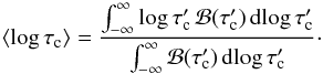
Appendix A: Excitation-like temperature in the ⟨3D⟩ model?
The referee raised the question why an average temperature based on its forth moment is suitable for constructing the ⟨3D⟩ model for comparison. Arguably, for representing spectral properties an average representative of the excitation properties related to the line formation might be the most suitable choice. In this section we want to emphasize that the choice of a suitable average is far from obvious, and our actual choice falls into the range of plausible choices – besides the argument brought already forward that an average based on the forth moment conserves the total flux well.
One may construct an excitation-like temperature Te in each
layer representing the mean population number of a particular energy level produced by
the temperature distribution in this layer via  (A.1)where
χ is the lower level energy, k is Boltzmann’s
constant, and b is an arbitrary exponent. The angular brackets
⟨.⟩ denote the spatial average. Relation (A.1) is motivated from the Saha-Boltzmann
equations governing the excitation and ionization in LTE. In this case,
b = 3/2 or
b = 5/2 (depending on whether the electron density
or electron pressure stays constant during temperature changes), and χ
might have to be identified with the difference between ionization energy and actual
level energy in case one deals with a minority species. Factors related to partition
functions are ignored. We want to derive an analytical estimate of
Te. To this end, we consider the temperature fluctuation
around the mean
(A.1)where
χ is the lower level energy, k is Boltzmann’s
constant, and b is an arbitrary exponent. The angular brackets
⟨.⟩ denote the spatial average. Relation (A.1) is motivated from the Saha-Boltzmann
equations governing the excitation and ionization in LTE. In this case,
b = 3/2 or
b = 5/2 (depending on whether the electron density
or electron pressure stays constant during temperature changes), and χ
might have to be identified with the difference between ionization energy and actual
level energy in case one deals with a minority species. Factors related to partition
functions are ignored. We want to derive an analytical estimate of
Te. To this end, we consider the temperature fluctuation
around the mean  as small
and derive the relation to lowest nontrivial order. Introducing for abbreviation the
parameter
as small
and derive the relation to lowest nontrivial order. Introducing for abbreviation the
parameter  we obtain for small x (
 ) the
expansion:
) the
expansion: ![\appendix \setcounter{section}{1} \begin{eqnarray} (1+x)^b {\rm e}^{-\frac{a}{1+x}} & \approx & {\rm e}^{-a}\,\left[1+\left\{a+b\right\} x^{\phantom{1}}\right.\nonumber\\ &&+\frac{1}{2} \left.\left\{a^2+ 2a (b-1) +b(b-1) \right\} x^2\right] \nonumber\\ &&+ \mathrm{O}[x^3]. \end{eqnarray}](/articles/aa/full_html/2013/11/aa21036-13/aa21036-13-eq156.png) (A.2)Introducing
(A.2)Introducing
 and
and
 we obtain
as second order
we obtain
as second order ![\appendix \setcounter{section}{1} \begin{eqnarray} \label{eqn:texpans} \xtmean{T^b {\rm e}^{-\frac{\chi}{kT}}} & \approx & \overline{T}^b {\rm e}^{-\frac{\chi}{k\overline{T}}} \left[1+\frac{1}{2} \left\{ \left(\frac{\chi}{k\overline{T}}\right)^2 \right.\right.\nonumber\\ &&+ \left.\left. 2 \frac{\chi}{k\overline{T}} (b-1) +b(b-1) \right\} \,\frac{\var{T}}{\overline{T}^2}\right] . \end{eqnarray}](/articles/aa/full_html/2013/11/aa21036-13/aa21036-13-eq159.png) (A.3)
(A.3) is the
variance of the temperature distribution. There is no linear term in ΔT
since ⟨ΔT⟩ = 0. Similarly, we obtain as first order
is the
variance of the temperature distribution. There is no linear term in ΔT
since ⟨ΔT⟩ = 0. Similarly, we obtain as first order ![\appendix \setcounter{section}{1} \begin{equation} \tex^b {\rm e}^{-\frac{\chi}{k\tex}} \approx \overline{T}^b {\rm e}^{-\frac{\chi}{k\overline{T}}} \left[ 1 + \left( \frac{\chi}{k\overline{T}} +b \right)\frac{\deltex}{\overline{T}}\right]. \label{eqn:teexpans} \end{equation}](/articles/aa/full_html/2013/11/aa21036-13/aa21036-13-eq163.png) (A.4)Combining the
expansions (A.3) and (A.4) results in
(A.4)Combining the
expansions (A.3) and (A.4) results in  (A.5)As an example, for
b = 0 (corresponding to the level population of a majority species)
and
(A.5)As an example, for
b = 0 (corresponding to the level population of a majority species)
and  the excitation temperature
is always greater than the (arithmetic) mean temperature in a given layer. Taking the
Sun as a typical example where
the excitation temperature
is always greater than the (arithmetic) mean temperature in a given layer. Taking the
Sun as a typical example where  in the line
forming region, this means that for lines with
χ > 1 eV it follows that
in the line
forming region, this means that for lines with
χ > 1 eV it follows that
 . However, the
difference between effective excitation temperature and mean temperature is generally
not large since the difference depends on the square of the temperature fluctuations.
. However, the
difference between effective excitation temperature and mean temperature is generally
not large since the difference depends on the square of the temperature fluctuations.
Average temperatures based on higher moments of the temperature also lead to changes
with respect to the mean temperature . One may ask
which moment is necessary to produce a temperature equal to the effective excitation
temperature. With the auxiliary formula
![\appendix \setcounter{section}{1} \begin{equation} (1+x)^n \approx 1 + n x + \frac{1}{2}n(n-1)x^2 +\mathrm{O}[x^3] \end{equation}](/articles/aa/full_html/2013/11/aa21036-13/aa21036-13-eq170.png) (A.6)we obtain
(A.6)we obtain
 (A.7)and
 (A.8)Since we demand
 we arrive
at
we arrive
at  (A.9)Combining the above
result with Eq. (A.5) we obtain for the
temperature moment n
(A.9)Combining the above
result with Eq. (A.5) we obtain for the
temperature moment n (A.10)The inequality
in relation (A.10) holds for
χ,b ≥ 0. Equation (A.10) illustrates that for already moderately high χ,
potentially enhanced by a non-zero b, one would need rather high
moments of the temperature to represent the effective excitation temperature correctly.
The consideration does not allow to identify an optimal n but
nevertheless illustrates that n = 4 is not an unreasonable choice
taking the excitation-like temperature as criterion.
(A.10)The inequality
in relation (A.10) holds for
χ,b ≥ 0. Equation (A.10) illustrates that for already moderately high χ,
potentially enhanced by a non-zero b, one would need rather high
moments of the temperature to represent the effective excitation temperature correctly.
The consideration does not allow to identify an optimal n but
nevertheless illustrates that n = 4 is not an unreasonable choice
taking the excitation-like temperature as criterion.
Appendix B: Base RGB versus tip RGB abundance corrections
As pointed out above, the abundance corrections derived in the present work for the red giants located near the base of the RGB (Teff = 5000 K, log g = 2.5, [M/H] = 0.0, −1, −2, −3) show little variation with wavelength, at least in the range 400−1600 nm. In contrast, Paper II demonstrated for a cooler red giant located near the tip of the RGB (Teff = 3600 K, log g = 1.0, [M/H] = 0.0) that the theoretical abundance corrections at 1600 nm were significantly smaller than those at optical wavelengths. In the following, we shall provide some basic explanation for the different wavelength dependence of the abundance corrections in these two type of giants.
As an example, we consider the formation of a weak fictitious high-excitation Fe ii line with χ = 6 eV, representative of the ionized atoms that show significant abundance corrections (at [M/H] = 0.0). In the case of the tip RGB giant, the abundance correction derived for this line is Δ3D−⟨ 3D ⟩ ≈ −0.4 dex at λ = 850 nm, and Δ3D−⟨ 3D ⟩ ≈ −0.02 dex at λ = 1600 nm. In the case of the less evolved giant of the present work, the corresponding numbers, for [M/H] = 0.0, are Δ3D−⟨ 3D ⟩ ≈ −0.06 dex (λ = 850 nm), and Δ3D−⟨ 3D ⟩ ≈ +0.02 dex (λ = 1600 nm). The metallicity dependence of the corrections is weak at λ = 850 nm and negligible at λ = 1600 nm (see Figs. 7 and 8). Since the corrections in the infrared are small for both type of giants, the remaining question is why the corrections in the red at λ = 850 nm are so much smaller in the “warm” giant than in the more evolved “cool” giant.
As in Paper II, the following considerations are restricted to vertical rays (disk-center intensity) in a single snapshot from the different 3D simulations. We focus here on the analysis of the “granulation correction”, Δ3D−⟨ 3D ⟩.
Mean height of formation, ⟨ log τc ⟩, of a fictitious Fe ii line with χ = 6 eV, at λ = 850 and 1600 nm, respectively, for the red giant model discussed in Paper II, and two of the CO5BOLD red giant models used in this work.
Appendix B.1: Temperature fluctuations on iso-surfaces of optical depth
We define the mean height of line formation as the center of gravity of the
equivalent width contribution function ℬ on the monochromatic
continuum optical depth scale τc:
 (B.1)For simplicity, we
use the contribution function of the ⟨3D⟩ atmosphere, corresponding to
ℬ2,2,2 in Paper II (Eq. (B.10)). The
results for the Fe ii line with χ = 6 eV are given in
Table B.1 for three different model
atmospheres at λ = 850 and 1600 nm, respectively. The mean height of
formation on the Rosseland optical depth scale,
⟨ log τRoss ⟩, is defined such that the average
temperature on the iso-surface
log τRoss = ⟨ log τRoss ⟩
is equal to the average temperature on the iso-surface
log τc = ⟨ log τc ⟩, which
we denote as ⟨ T ⟩ line. For all three models listed in
Table B.1, the infrared line forms in
significantly deeper atmospheric layers than the red line. This is the expected result
since the continuum opacity is mainly due to H− and shows a local maximum
near λ 850 nm, and a minimum close to λ 1600 nm.
In the metal-poor giant, the line contribution function is more asymmetric and extends
towards higher atmospheric layers than in the solar metallicity giant at the same
Teff and log g. This is related to the
fact that the continuum opacity decreases more steeply with height in the metal-poor
atmosphere (due to the reduced electron pressure). For given stellar parameters, the
mean height of line formation is therefore shifted towards higher atmospheric layers
at low metallicity.
(B.1)For simplicity, we
use the contribution function of the ⟨3D⟩ atmosphere, corresponding to
ℬ2,2,2 in Paper II (Eq. (B.10)). The
results for the Fe ii line with χ = 6 eV are given in
Table B.1 for three different model
atmospheres at λ = 850 and 1600 nm, respectively. The mean height of
formation on the Rosseland optical depth scale,
⟨ log τRoss ⟩, is defined such that the average
temperature on the iso-surface
log τRoss = ⟨ log τRoss ⟩
is equal to the average temperature on the iso-surface
log τc = ⟨ log τc ⟩, which
we denote as ⟨ T ⟩ line. For all three models listed in
Table B.1, the infrared line forms in
significantly deeper atmospheric layers than the red line. This is the expected result
since the continuum opacity is mainly due to H− and shows a local maximum
near λ 850 nm, and a minimum close to λ 1600 nm.
In the metal-poor giant, the line contribution function is more asymmetric and extends
towards higher atmospheric layers than in the solar metallicity giant at the same
Teff and log g. This is related to the
fact that the continuum opacity decreases more steeply with height in the metal-poor
atmosphere (due to the reduced electron pressure). For given stellar parameters, the
mean height of line formation is therefore shifted towards higher atmospheric layers
at low metallicity.
Table B.1 also gives the relative rms temperature fluctuation δTrms, both on the τc and the τRoss iso-surface defining the center of the line forming region. The full depth-dependence of δTrms is shown in Fig. B.1. We find that, at any given mean temperature, δTrms is always systematically larger on τ850 iso-surfaces than on τ1600 iso-surfaces. This is a consequence of the lower temperature sensitivity of the continuum opacity at λ 850 nm compared to λ 1600 nm. The Rosseland opacity has an intermediate T sensitivity, and hence the amplitude of the temperature fluctuations lies between the values at λ 850 nm and λ 1600 nm. This behavior is seen for all model atmospheres considered here, but is particularly pronounced in the cool giant. The general picture emerging from Table B.1 and Fig. B.1 indicates that the temperature fluctuations in the line forming layers are largest in the cool giant, and smallest in the warmer metal-poor giant. The 3D abundance corrections are therefore expected to be potentially larger for giants near the tip than near the base of the RGB. This is confirmed by the more detailed analysis below.
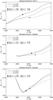 |
Fig. B.1 Amplitude of the relative rms temperature fluctuations δTrms/ ⟨ T ⟩ versus the average temperature ⟨ T ⟩, evaluated on different iso-optical depth surfaces: τ850 (solid), τ1600 (dashed), τRoss (dotted). Filled circles indicate the values at the mean height of line formation at λ 850 nm and λ 1600 nm, respectively, as given in Table B.1. |
Appendix B.2: Opacity fluctuations and abundance corrections
We recall that, in the weak line limit, the abundance correction
Δ3D−⟨ 3D ⟩ can be computed as  (B.2)where
W 3D and W⟨ 3D ⟩ denote the
line equivalent width obtained from the 3D and the ⟨3D⟩ model, respectively, for the
same atomic line parameters and elemental abundance (see Paper II, Appendix B). With
the help of the equivalent width contribution function ℬ, we can write the ratio of
equivalent widths as
(B.2)where
W 3D and W⟨ 3D ⟩ denote the
line equivalent width obtained from the 3D and the ⟨3D⟩ model, respectively, for the
same atomic line parameters and elemental abundance (see Paper II, Appendix B). With
the help of the equivalent width contribution function ℬ, we can write the ratio of
equivalent widths as  (B.3)with the mixed
contribution function
(B.3)with the mixed
contribution function  (B.4)as
defined in Paper II, Eq. (B.10). Subscripts 2 and 3 refer to the ⟨3D⟩ model and the 3D
model, respectively.
(B.4)as
defined in Paper II, Eq. (B.10). Subscripts 2 and 3 refer to the ⟨3D⟩ model and the 3D
model, respectively.
To isolate the role of the line opacity fluctuations for the
abundance corrections, we consider the ratio  (B.5)where
we have defined the local amplification factor
(B.5)where
we have defined the local amplification factor
 as
as  (B.6)According to
Eq. (B.5), the equivalent width
ratio ℛ2,3,2 can be expressed as an
average of the amplification factor
over optical depth with weighting function
ℬ2,2,2. Figure B.2 (left column) shows the depth dependence of
at both wavelengths for the three red giant models under consideration, together with
the weighting function ℬ2,2,2 and the
resulting values of ℛ2,3,2. The largest
3D effects are found in the cool giant. The reason is twofold: (i) the amplitude of
the temperature fluctuations in the line forming layers of the cool giant is
significantly higher than in the warmer giants (see above); (ii) the Fe ii
ionization fraction is strongly variable in the atmosphere of the cool giant,
especially in the layers where the λ 850 nm line forms, while
Fe ii is always the dominating ionization stage in the warmer giants. Both
factors enhance the nonlinearity of the line opacity fluctuations in the cool giant,
and lead to the pronounced 3D abundance corrections.
(B.6)According to
Eq. (B.5), the equivalent width
ratio ℛ2,3,2 can be expressed as an
average of the amplification factor
over optical depth with weighting function
ℬ2,2,2. Figure B.2 (left column) shows the depth dependence of
at both wavelengths for the three red giant models under consideration, together with
the weighting function ℬ2,2,2 and the
resulting values of ℛ2,3,2. The largest
3D effects are found in the cool giant. The reason is twofold: (i) the amplitude of
the temperature fluctuations in the line forming layers of the cool giant is
significantly higher than in the warmer giants (see above); (ii) the Fe ii
ionization fraction is strongly variable in the atmosphere of the cool giant,
especially in the layers where the λ 850 nm line forms, while
Fe ii is always the dominating ionization stage in the warmer giants. Both
factors enhance the nonlinearity of the line opacity fluctuations in the cool giant,
and lead to the pronounced 3D abundance corrections.
 |
Fig. B.2 Depth dependence of amplification factors
|
Next we consider the combined effect of line and continuum opacity
fluctuations. For this purpose, we have to evaluate the amplification
factor  :
:
 (B.7)where
ηℓ = κℓ/κc
is the ratio of line to continuum opacity. Again, the effective amplification factor
ℛ2,3,3 is obtained as the average of
the local amplification factor
over optical depth with weighting function
ℬ2,2,2. The result is shown in
Fig. B.2 (right column). Obviously, the line
and the continuum opacity are correlated in the sense that both increase with
temperature, such that the fluctuation amplitude of their ratio,
ηℓ, is always lower than the
fluctuation amplitude of the line opacity,
κℓ. Hence,
ℛ2,3,3 is smaller than
ℛ2,3,2. For the warmer giants, the
reduction of ℛ is of similar magnitude for both wavelengths,
log (ℛ2,3,3/ℛ2,3,2) ≈ −0.05
dex. For the cool giant, however, the reduction factor is much smaller at
λ 850 nm (≈−0.01 dex) than at λ 1600 nm
(≈−0.11 dex), further increasing the difference between the 3D corrections derived
for the two wavelengths.
(B.7)where
ηℓ = κℓ/κc
is the ratio of line to continuum opacity. Again, the effective amplification factor
ℛ2,3,3 is obtained as the average of
the local amplification factor
over optical depth with weighting function
ℬ2,2,2. The result is shown in
Fig. B.2 (right column). Obviously, the line
and the continuum opacity are correlated in the sense that both increase with
temperature, such that the fluctuation amplitude of their ratio,
ηℓ, is always lower than the
fluctuation amplitude of the line opacity,
κℓ. Hence,
ℛ2,3,3 is smaller than
ℛ2,3,2. For the warmer giants, the
reduction of ℛ is of similar magnitude for both wavelengths,
log (ℛ2,3,3/ℛ2,3,2) ≈ −0.05
dex. For the cool giant, however, the reduction factor is much smaller at
λ 850 nm (≈−0.01 dex) than at λ 1600 nm
(≈−0.11 dex), further increasing the difference between the 3D corrections derived
for the two wavelengths.
The similarity of ℛ2,3,2 and
ℛ2,3,3 for the
λ 850 nm line in the cool giant is implied by the similarity of the
local amplification factors
and
in the line forming region. The reason for this behavior can be traced back to the low
temperature sensitivity of the continuum opacity in the temperature range 4000 K
< T < 5000 K (cf.
Fig. B.2. in Paper II), which coincides with the formation region of this line (see
blue weighting function in the upper panels of Fig. B.2). For the warmer giant with solar metallicity, a similar “plateau” in
the κc versus T relation is found in the
same temperature range. However, in this giant the λ 850 nm line
forms at higher temperatures (see blue weighting function in the middle panels of
Fig. B.2), and the temperature sensitivity of
κc is thus comparable at both wavelengths. Remarkably,
the “plateau” in the κc versus T relation
is not seen in the metal-poor giants. Presumably, the “plateau” is related to the
transition from a hydrogen to a metal dominated electron source, the latter being
negligible in a metal-poor atmosphere.
Finally, we have also evaluated the full 3D corrections ℛ3,3,3, marked by star symbols in Fig. B.2 (right panels). The additional effect of the fluctuations of the source function gradient uc is only significant in the cool giant, and increases the dichotomy between the corrections at λ 850 and 1600 nm even further. A similar behavior was found for the Fe ii line with χ = 10 eV investigated in Paper II.
In summary, the 3D corrections for high-excitation lines of ions at wavelengths near λ 850 nm are significantly larger in the cool tip RGB giant discussed in Paper II than in the warmer giants near the base of the RGB studied in the present work because, in the cool giant, the lines form in a region where (i) the temperature fluctuations are larger, (ii) the temperature sensitivity of the continuum opacity is particularly low, and (iii) the ionization fraction of typical ions like Fe ii varies considerably, thus enhancing the temperature sensitivity of the line opacity.
Appendix C: Formation of molecular lines
Horizontal temperature fluctuations play an essential role in defining abundance corrections for the molecules. Firstly, they are larger in the 3D hydrodynamical models at lower metallicity (cf. Figs. 1, 2), which leads to the highest molecular number density and line opacity fluctuations in the lowest metallicity models. Secondly, in a model of a given metallicity different molecules form at different optical depths which are characterized by different amplitude of the horizontal temperature fluctuations. For example, CO formation occupies the outermost range in terms of Rosseland optical depth of all molecules studied here (Fig. C.2). Consequently, its lines form in the atmospheric layers characterized by the largest horizontal temperature fluctuations (cf. Fig. 2) in comparison to those in the layers where other molecules form. The fluctuations of the line opacity is therefore largest in the case of CO in the 3D model at [M/H] = −3.0, which is part of the explanation of the large abundance corrections for CO. However, further factors are important.
 |
Fig. C.1 Number density of different molecules, normalized to the total number density of carbon, plotted as a function of the Rosseland optical depth in the 1D LHD model at [M/H] = −3.0. |
According to Paper II, the number density of molecules per unit mass (calculated as
Xi = Ni/ρ,
here ρ is the mass density) can be computed using the following
Saha-like equation  (C.1)where
QAB is the partition function of the molecule AB,
XA and XB are number densities
per unit mass of the constituent species A and B, with their partition functions
UA and UB, respectively, mass
of the molecule mAB, its dissociation energy
D0, and temperature, T. The number
densities of the molecules studied here are shown in Fig. C.1 plotted versus Rosseland optical depth in the 1D
LHD model at [M/H] = −3.0 (number
densities are normalized to the total number density of carbon nuclei,
XAB/ ∑ XC).
Qualitatively, the situation is very similar to that in the cool red giant studied by
Paper II: because the abundance of oxygen is higher than that of carbon, most of the
available C is locked into CO beyond log τRoss ~ −0.5. In
the deeper atmosphere, the molecules are quickly destroyed due to dissociation.
(C.1)where
QAB is the partition function of the molecule AB,
XA and XB are number densities
per unit mass of the constituent species A and B, with their partition functions
UA and UB, respectively, mass
of the molecule mAB, its dissociation energy
D0, and temperature, T. The number
densities of the molecules studied here are shown in Fig. C.1 plotted versus Rosseland optical depth in the 1D
LHD model at [M/H] = −3.0 (number
densities are normalized to the total number density of carbon nuclei,
XAB/ ∑ XC).
Qualitatively, the situation is very similar to that in the cool red giant studied by
Paper II: because the abundance of oxygen is higher than that of carbon, most of the
available C is locked into CO beyond log τRoss ~ −0.5. In
the deeper atmosphere, the molecules are quickly destroyed due to dissociation.
From Eq. (C.1) one can expect rather different temperature sensitivity of the number densities of different molecules. Indeed, this is clearly seen in Fig. C.3 where we show number (normalized) densities of CO, CN, CH, C2, NH and OH in the 3D model ([M/H] = −3.0) at different levels of constant Rosseland optical depths, plotted versus inverse temperature θ = 5040/T. It is obvious that CO is significantly more sensitive to changes in T than the other molecules, essentially due to the high dissociation energy of CO, D0 = 11.1 eV. In fact, the temperature sensitivity of the molecular number densities scales with D0 in the hotter parts of the atmosphere where T ≳ 4000 K. In the cooler regions, however, where almost all carbon is locked up in CO and atomic carbon is a minority species, the temperature dependence of the number density of the other carbon-bearing molecules is reversed: here a temperature increase leads to the destruction of CO, and in turn, to a larger concentration of atomic carbon that enables an enhanced formation of carbon-bearing molecules. Carbon-free molecules
do not show this anomalous behavior at low temperature (see lower panels of Fig. C.3).
Since the line opacity is directly proportional to XAB, larger fluctuations of the number densities should lead to larger fluctuations and larger nonlinearities in the line opacities, and thus to larger abundance corrections. This is basically what one sees in case of CO: the broadest range of fluctuations in the case of CO leads to the largest abundance corrections amongst all molecules investigated here.
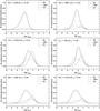 |
Fig. C.2 Equivalent width contribution function (flux) of weak (W ≤ 0.5 pm) artificial molecular lines of CO, CN, CH, C2, NH, OH (top left to bottom right) with lower level excitation potential χ = 0 eV in the full 3D, average ⟨3D⟩, and 1D model atmospheres with metallicity [M/H] = −3.0. Contribution functions were normalized to the equivalent width of the line computed using 3D models. |
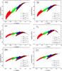 |
Fig. C.3 Normalized number densities of molecules CO, CN, CH, C2, NH, OH (top left to bottom right) in the 3D model atmosphere ([M/H] = −3.0) plotted at different levels of constant Rosseland optical depth (identified by color) as a function of inverse temperature θ = 5040/T. |
Interestingly, in the case of cool red giant studied in Paper II, the abundance corrections were largest for C2. In contrast, the abundance corrections for C2 obtained in this work are in fact smallest amongst all molecules. A closer look at the dependence of C2 number density on temperature reveals that XC2 increases steeply up to T ~ 4000 K and then decreases towards the higher temperatures (Fig. C.3, middle right). This is because the formation of C2 is tightly coupled to that of CO, as explained above, and makes the number density of C2 extremely sensitive to changes in temperature at low T. In the cool red giant analyzed by Paper II the atmosphere is significantly cooler and the C2 line forms entirely the lower temperature regime where X(C2) is highly sensitive to the temperature fluctuations, leading to the largest abundance corrections for C2. In the warmer red giant studied here, however, the C2 line forms in the transition region between both temperature regimes, such that the amplitude of the fluctuations is limited and their net effect on the abundance corrections is much smaller.
NH (D0 = 3.5 eV) and OH (D0 = 4.4 eV) have similar molecular properties and line formation regions. The 3D abundance correction is slightly more negative for OH because this molecule has a somewhat higher dissociation energy. The correction for CN (D0 = 7.8 eV) falls in the same range, although this molecule has a much higher dissociation energy. Again, the explanation for this unexpected behavior is related to the change of sign in the temperature sensitivity of the number density of CN in the line forming region (log τRoss = −2), due to the coupling with CO at low temperatures. The coupling with CO is missing in the case of carbon-free molecules NH and OH, where the slope ∂log N/∂θ is therefore essentially constant over the whole temperature range (see Fig. C.3, lower panels).
Acknowledgments
We thank the anonymous referee for very comprehensive comments and suggestions which helped to improve the paper significantly. This work was supported by grant from the Research Council of Lithuania (MIP-101/2011). H.G.L., and E.C. acknowledge financial support by the Sonderforschungsbereich SFB 881 “The Milky Way System” (subproject A4) of the German Research Foundation (DFG). A.K. and H.G.L. acknowledge financial support from the Sonderforschungsbereich SFB 881 “The Milky Way System” (subproject A4) of the German Research Foundation (DFG) that allowed exchange visits between Vilnius and Heidelberg. P.B. and A.K. acknowledge support from the Scientific Council of the Observatoire de Paris and the Research Council of Lithuania (MOR-48/2011) that allowed exchange visits between Paris and Vilnius.
References
- Asplund, M., Nordlund, Å., Trampedach, R., Allen de Prieto, C., & Stein, R. F. 2000, A&A, 359, 729 [NASA ADS] [Google Scholar]
- Asplund, M., Grevesse, N., & Sauval, A. J. 2005, ASPC, 336, 25 [Google Scholar]
- Behara, N. T., Bonifacio, P., Ludwig, H.-G., et al. 2010, A&A, 513, A72 [NASA ADS] [CrossRef] [EDP Sciences] [Google Scholar]
- Böhm-Vitense, E. 1958, Z. Astrophys., 46, 108 [Google Scholar]
- Brott, I., & Hauschildt, P. H. 2005, in The Three-Dimensional Universe with Gaia, eds. C. Turon, K. S. O’Flaherty, & M. A. C. Perryman, ESA SP 576, 565 [Google Scholar]
- Caffau, E., Ludwig, H.-G., Steffen, M., et al. 2008, A&A, 488, 1031 [CrossRef] [EDP Sciences] [Google Scholar]
- Caffau, E., Maiorca, E., Bonifacio, P., et al. 2009, A&A, 498, 877 [NASA ADS] [CrossRef] [EDP Sciences] [Google Scholar]
- Caffau, E., Ludwig, H.-G., Steffen, M., Freytag, B., & Bonifacio, P. 2011, Sol. Phys., 268, 255 [NASA ADS] [CrossRef] [Google Scholar]
- Canuto, V. M., & Mazzitelli, I. 1991, ApJ, 370, 295 [NASA ADS] [CrossRef] [Google Scholar]
- Castelli, F., & Kurucz, R. L. 2003, in Modeling of Stellar Atmospheres, eds. N. E. Piskunov, W. W. Weiss, & D. F. Gray, IAU Symp. Proc., 210, A20 (CD-ROM); synthetic spectra available at http://cfaku5.cfa.harvard.edu/grids [Google Scholar]
- Collet, R., Asplund, M., & Trampedach, R. 2007, A&A, 469, 687 [NASA ADS] [CrossRef] [EDP Sciences] [Google Scholar]
- Collet, R., Hayek, W., Asplund, M., et al. 2011, A&A, 528, A32 [NASA ADS] [CrossRef] [EDP Sciences] [Google Scholar]
- Dobrovolskas, V., Kučinskas, A., Ludwig, H.-G., et al. 2010, in Proc. of 11th Symposium on Nuclei in the Cosmos, PoS(NIC XI)288 [Google Scholar]
- Freytag, B., Steffen, M., Ludwig, H.-G., et al. 2012, J. Comp. Phys., 231, 919 [Google Scholar]
- GonzálezHernández, J. I., Bonifacio, P., Caffau, E., et al. 2009, A&A, 505, 13 [Google Scholar]
- Gustafsson, B., Edvardsson, B., Eriksson, K., et al. 2008, A&A, 486, 951 [NASA ADS] [CrossRef] [EDP Sciences] [Google Scholar]
- Ivanauskas, A., Kučinskas, A., Ludwig, H.-G., & Caffau, E. 2010, in Proc. of 11th Symposium on Nuclei in the Cosmos, PoS(NIC XI)290 [Google Scholar]
- Kučinskas, A., Steffen, M., Ludwig, H.-G., et al. 2013, A&A, 549, A14 (Paper II) [NASA ADS] [CrossRef] [EDP Sciences] [Google Scholar]
- Ludwig, H.-G. 1992, Ph.D. Thesis, University of Kiel [Google Scholar]
- Ludwig, H.-G., & Kučinskas, A. 2012, A&A, 547, A118 (Paper I) [NASA ADS] [CrossRef] [EDP Sciences] [Google Scholar]
- Ludwig, H.-G., & Steffen, M. 2012, in Red giants as probes of the structure and evolution of the Milky Way (Berlin: Springer-Verlag), Ap&SS, Proc., 2, 125 [Google Scholar]
- Ludwig, H.-G., Jordan, S., & Steffen, M. 1994, A&A, 284, 105 [NASA ADS] [Google Scholar]
- Ludwig, H.-G., Caffau, E., Steffen, M., et al. 2009, Mem. Soc. Astron. Italiana, 80, 711 [Google Scholar]
- Mihalas, D. 1978, Stellar Atmospheres, 2nd ed. (San Francisco: Freeman & Co.) [Google Scholar]
- Nordlund, Å. 1982, A&A, 107, 1 [Google Scholar]
- Steffen, M., & Holweger, H. 2003, in Modelling of Stellar Atmospheres, IAU Symp. Proc., 210, 15 [Google Scholar]
- Stein, R. F., & Nordlund, Å. 1998, ApJ, 499, 914 [Google Scholar]
- Vögler, A. 2004, A&A, 421, 755 [NASA ADS] [CrossRef] [EDP Sciences] [Google Scholar]
- Vögler, A., Bruls, J. H. M. J., & Schüssler, M. 2004, A&A, 421, 741 [NASA ADS] [CrossRef] [EDP Sciences] [Google Scholar]
All Tables
Mean height of formation, ⟨ log τc ⟩, of a fictitious Fe ii line with χ = 6 eV, at λ = 850 and 1600 nm, respectively, for the red giant model discussed in Paper II, and two of the CO5BOLD red giant models used in this work.
All Figures
|
Fig. 1 Upper panel: temperature profiles in the red giant model with Teff/log g/ [M/H] = 4970/2.5/0.0, plotted versus the Rosseland optical depth, τRoss, and shown for the following model atmospheres: 3D (density plot), ⟨3D⟩ (dashed line), and 1D (solid line). Horizontal bars mark the approximate location of the Fe I and Fe II line formation regions in the 3D (black) and 1D (blue) atmosphere models, at λ = 400 nm and χ = 0 and 6 eV (bars mark the regions where the equivalent width, W, of a given spectral line grows from 5% to 95% of its final value). Lower panel: rms horizontal temperature fluctuations in the 3D model (solid line), and difference between the temperature profiles of the ⟨3D⟩ and 1D models (dashed line), shown as functions of the Rosseland optical depth. In both panels, all quantities related to the 3D and ⟨3D⟩ models were obtained using the subset of twenty 3D model snapshots utilized in the 3D spectral line synthesis calculations (see Sect. 2.1). |
| In the text | |
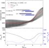 |
Fig. 2 Same as in Fig. 1 but for the red giant model with Teff/log g/ [M/H] = 5020/2.5/−3.0. |
| In the text | |
|
Fig. 4 Abundance corrections for spectral lines of neutral atoms plotted versus metallicity at λ = 850 nm: Δ3D−⟨ 3D ⟩ (left column), Δ⟨ 3D ⟩ −1D (middle column), and Δ3D−1D (right column). Corrections are given at several different excitation potentials, as indicated on the right side of each row. Abundance corrections at λ = 400 nm and λ = 1600 nm (Figs. 3 and 5, respectively) are available in the online version only. |
| In the text | |
|
Fig. 7 Same as in Fig. 3 but for lines of ionized atoms, plotted versus metallicity and excitation potential at λ = 850 nm. Abundance corrections at λ = 400 nm and λ = 1600 nm (Figs. 6 and 8, respectively) are available in the online version only. |
| In the text | |
|
Fig. 10 Same as in Fig. 3 but for molecular lines plotted versus metallicity and excitation potential at λ = 850 nm. Abundance corrections at λ = 400 nm and λ = 1600 nm (Figs. 9 and 11, respectively) are available in the online version only. |
| In the text | |
|
Fig. 12 Top panel: temperature profiles of the average ⟨3D⟩ model (Teff = 5020 K, log g = 2.5, and [M/H] = −3.0) calculated with scattering treated as true absorption (red solid line) and with scattering opacity neglected at small τRoss (red dashed line). Black lines mark the 5th and 95th percentiles of the temperature distribution in the 3D model with scattering treated as true absorption (solid lines) and scattering opacity neglected in optically thin regions (dashed lines). Horizontal bars indicate the approximate location where lines of several trace elements form at λ = 400 nm and χ = 0 and 4 eV and of the CO molecule at λ = 400 nm and χ = 0 and 3 eV (bars mark the regions where the equivalent width, W, of a given spectral line grows from 5% to 95% of its final value). Bottom panel: difference in the temperature profiles corresponding to the average ⟨3D⟩ models calculated with the two different treatments of scattering. |
| In the text | |
|
Fig. 13 Abundance corrections obtained for selected elements and for the CO molecule with the model atmospheres computed using different treatments of scattering (plotted versus the excitation potential χ, for lines at λ = 400 nm). For each element, two cases are shown: (a) with scattering treated as true absorption (solid lines), and (b) with scattering opacity neglected in the optically thin regions (dashed lines). Atmospheric parameters of the model atmospheres are Teff = 5020, log g = 2.5, and [M/H] = −3.0. Three types of abundance corrections are shown: Δ3D−⟨ 3D ⟩ (left column), Δ⟨ 3D ⟩ −1D (middle column), and Δ3D−1D (right column). |
| In the text | |
|
Fig. 14 Velocity profiles of the LHD models (red/gray lines) at [M/H] = 0.0 (top panel) and [M/H] = −3.0 (bottom panel) computed using three different mixing-length parameters, αMLT = 1,1.5,2.0. Vertical and horizontal velocity profiles of the average ⟨3D⟩ model (computed on the log τRoss iso-surfaces are shown as solid and dot-dashed black lines, respectively. |
| In the text | |
|
Fig. 15 Abundance corrections for two fictitious lines of neutral iron (χ = 0 and 6 eV) and one of ionized iron (χ = 6 eV) at 400 nm, plotted versus the mixing-length parameter αMLT used with the 1D LHD model atmospheres at [M/H] = 0.0 (top row) and [M/H] = −3.0 (bottom row). Three types of abundance corrections are shown: Δ3D−⟨ 3D ⟩ (left column), Δ⟨ 3D ⟩ −1D (middle column), and Δ3D−1D (right column). Note that Δ3D−⟨ 3D ⟩ abundance correction is not influenced by the choice of αMLT (there is no comparison 1D model atmosphere involved); we nevertheless show all three abundance corrections to provide an indication of the absolute size of abundance corrections involved and the range of their variations with αMLT. |
| In the text | |
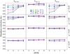 |
Fig. 3 Same as in Fig. 4 but at λ = 400 nm. |
| In the text | |
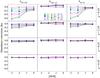 |
Fig. 5 Same as in Fig. 4 but at λ = 1600 nm. |
| In the text | |
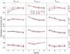 |
Fig. 6 Same as in Fig. 7 but at λ = 400 nm. |
| In the text | |
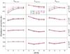 |
Fig. 8 Same as in Fig. 7 but at λ = 1600 nm. |
| In the text | |
 |
Fig. 9 Same as in Fig. 10 but at λ = 400 nm. |
| In the text | |
 |
Fig. 11 Same as in Fig. 10 but at λ = 1600 nm. |
| In the text | |
|
Fig. B.1 Amplitude of the relative rms temperature fluctuations δTrms/ ⟨ T ⟩ versus the average temperature ⟨ T ⟩, evaluated on different iso-optical depth surfaces: τ850 (solid), τ1600 (dashed), τRoss (dotted). Filled circles indicate the values at the mean height of line formation at λ 850 nm and λ 1600 nm, respectively, as given in Table B.1. |
| In the text | |
|
Fig. B.2 Depth dependence of amplification factors
|
| In the text | |
|
Fig. C.1 Number density of different molecules, normalized to the total number density of carbon, plotted as a function of the Rosseland optical depth in the 1D LHD model at [M/H] = −3.0. |
| In the text | |
|
Fig. C.2 Equivalent width contribution function (flux) of weak (W ≤ 0.5 pm) artificial molecular lines of CO, CN, CH, C2, NH, OH (top left to bottom right) with lower level excitation potential χ = 0 eV in the full 3D, average ⟨3D⟩, and 1D model atmospheres with metallicity [M/H] = −3.0. Contribution functions were normalized to the equivalent width of the line computed using 3D models. |
| In the text | |
|
Fig. C.3 Normalized number densities of molecules CO, CN, CH, C2, NH, OH (top left to bottom right) in the 3D model atmosphere ([M/H] = −3.0) plotted at different levels of constant Rosseland optical depth (identified by color) as a function of inverse temperature θ = 5040/T. |
| In the text | |
Current usage metrics show cumulative count of Article Views (full-text article views including HTML views, PDF and ePub downloads, according to the available data) and Abstracts Views on Vision4Press platform.
Data correspond to usage on the plateform after 2015. The current usage metrics is available 48-96 hours after online publication and is updated daily on week days.
Initial download of the metrics may take a while.