| Issue |
A&A
Volume 557, September 2013
|
|
|---|---|---|
| Article Number | A34 | |
| Number of page(s) | 8 | |
| Section | Extragalactic astronomy | |
| DOI | https://doi.org/10.1051/0004-6361/201321666 | |
| Published online | 20 August 2013 | |
A method for quantifying the gamma-ray burst bias. Application in the redshift range of 0–1.1
1 Aix Marseille Université, CNRS, LAM (Laboratoire d’Astrophysique de Marseille) UMR 7326, 13388 Marseille, France
e-mail: This email address is being protected from spambots. You need JavaScript enabled to view it.
2 INAF, IASF Milano, via E. Bassini 15, 20133 Milano, Italy
3 Laboratoire AIM, CEA/DSM/IRFU, CNRS, Université Paris-Diderot, 91190 Gif, France
4 Institut d’Astrophysique de Paris, UMR 7095 CNRS, Univ. P. & M. Curie, 98bis Bd. Arago, 75104 Paris, France
5 GEPI, Observatoire de Paris, CNRS, Univ. Paris Diderot, 5 place Jules Janssen, 92190 Meudon, France
6 Max Planck Institute for extraterrestrial Physics, PO Box 1312, Giessenbachstr., 85741 Garching, Germany
Received: 8 April 2013
Accepted: 2 July 2013
Abstract
Context. Long gamma-ray bursts (LGRBs) are related to the final stages of evolution of very massive stars. As such, they should follow the star formation rate (SFR) of galaxies. We can use them to probe for star-forming galaxies in the distant universe following this assumption. The relation between the rate of LGRBs in a given galaxy and its SFR (which we call the LGRB bias) may however be complex, as we have good indications that the LGRB hosts are not perfect analogues to the general population of star-forming galaxies.
Aims. In this work, we try to quantify how the LGRB bias depends on physical parameters of their host galaxy, such as SFR or stellar mass. These trends may reveal more fundamental properties such as the role of the metallicity of LGRBs and of their progenitors .
Methods. We propose an empirical method based on the comparison of stellar mass functions (and SFR distributions) of LGRB hosts and of star-forming galaxies to find how the bias depends on the stellar mass or the SFR.
Results. By applying this method to a sample of LGRB hosts at redshifts lower than 1.1, where the properties of star-forming galaxies are fairly well established and where the properties of LGRB host galaxies can be deduced from observations (limiting ourselves to stellar masses higher than 109.25 M⊙ and SFR higher than ~1.8 M⊙ yr-1), we find that the LGRB bias depends on both the stellar mass and SFR. We find that the bias decreases with the SFR; that is, we see no preference for highly star-forming galaxies, once we account for the higher number of massive stars in galaxies with larger SFR. We do not find any trend with the specific star formation rate (SSFR), but the dynamical range in SSFR in our study is narrow. Through an indirect method, we relate these trends to a possible decrease in the LGRBs rate / SFR ratio with the metallicity.
Conclusions. The method we propose suggests trends that may be useful to constrain models of LGRB progenitors, showing a clear decrease in the LGRB bias with the metallicity. This is promising for the future as the number of LGRB hosts studied will increase.
Key words: gamma-ray burst: general / galaxies: luminosity function, mass function / galaxies: star formation / galaxies: evolution / galaxies: high-redshift
© ESO, 2013
1. Introduction
The relation between long duration gamma-ray bursts (LGRBs) and the explosion of (very) massive stars is now established (e.g. Woosley & Bloom 2006). Since massive stars are short-lived, it is often concluded that LGRBs can be used to trace star formation up to very high redshift (e.g. Kistler et al. 2009; Robertson & Ellis 2012)1. Owing to the relation between LGRBs and massive stars, it is possible to write that the rate of LGRBs in a galaxy is a simple function of its star formation rate (SFR):  (1)where b is the LGRB bias. By this, we do not assume a priori that LGRB hosts are necessarily biased with respect to field galaxies, but we define and study the relation between the two rates (SFR and LGRB rate). In an ideal case (assuming a constant initial mass function), the fraction of massive stars giving rise to LGRBs would be universal, and b would be a constant. This assumption is often implicitly made when the luminosity functions of normal star-forming galaxies and LGRB host galaxies are compared (e.g. Le Floc’h et al. 2003; Basa et al. 2012). If b were really a universal constant, the LGRB host galaxies however should be similar to galaxies selected by their SFR, and thus similar to star-forming galaxies (SFGs). On the contrary, it was found that host galaxies at low redshifts have lower luminosities and bluer colours (Le Floc’h et al. 2003; Fruchter et al. 1999); lower stellar masses (e.g. Castro Cerón et al. 2010, see however Perley et al. 2003; Krühler et al. 2011); lower metallicities (Modjaz et al. 2008; Levesque et al. 2010a; Han et al. 2010); higher [Ne III] fluxes indicating very massive star formation (Bloom et al. 1998); more irregular morphology (Fruchter et al. 2006); or larger specific star formation rates (SSFRs; Christensen et al. 2004; Castro Cerón et al. 2006) than SFGs.
Other approaches indicate that the bias must evolve with redshift and that the LGRB rate is enhanced at high redshift with respect to the SFR (e.g. Daigne et al. 2006; Kistler et al. 2009; Virgili et al. 2011). These studies combine hypothetical variations of the bias b with models of the intrinsic evolution of galaxies from the highest redshifts to the present day and with the sensitivity of the instruments used to detect LGRBs. Their predictions are then compared to the observed redshift distribution of LGRBs (e.g. Salvaterra et al. 2012; Robertson & Ellis 2012; Elliott et al. 2012) or to other quantities, such as the luminosity distribution (Wolf & Podsiadlowski 2007), or the mass function of LGRB host galaxies (e.g. Kocevski et al. 2009). This variation in the LGRB bias with the redshift is sometimes written under the form of  (2)with n usually found between n = 0.4 and 1.2 (e.g. Robertson & Ellis 2012; Qin et al. 2010; Kistler et al. 2009). Since a star at the end of its life does not know its redshift, this evolution should be ascribed to changes in physical properties of galaxies varying with cosmic time. The culprits could be the initial mass function (changing the relative number of massive stars that could evolve into a LGRB in proportion to the SFR integrated over the full initial mass function as for other SFR tracers) or the metallicity. A possible effect of metallicity on the occurrence of a LGRB has some theoretical support (e.g. MacFadyen & Woosley 1999; Woosley & Heger 2006; Georgy et al. 2009; Podsiadlowski et al. 2010). A metallicity effect was considered under several forms (including cut-offs) and used to interpret various sets of data (e.g. Wolf & Podsiadlowski 2007; Modjaz et al. 2008; Graham & Fruchter 2013).
We adopt the point of view that host galaxies should form a subset of SFGs and that the differences between this subset and the whole population of SFGs is due to a variation in b with physical properties (deciding which of these galaxies hosts LGRBs or not). These relations should also be responsible for the apparent redshift evolution of b when integrated over the whole population of galaxies. We propose a relatively direct method to search for these effects. We quantify the differences between LGRB host galaxies and SFGs (in terms of the distribution functions of their stellar masses and SFR) to measure how b depends on these and other quantities (such as the metallicity). Section 2 proposes the formalism and methodology to achieve this goal applied to the redshift range 0 to 1.1 for this study. The sample we selected to test our method is presented in Sect. 3, while our results are described in Sect. 4. In Sect. 5, we discuss the main limit of our approach (the apparent dichotomy between SFGs and LGRB hosts). Our conclusions are summarized in Sect. 6.
2. Formalism
2.1. Variation in the LGRB bias with the SFR
The SFR distribution φSFG provides the number of star-forming galaxies with a given SFR. This function is nowadays measured in a number of deep surveys; the SFR is derived, for instance, from the rest-frame UV, the far-infrared luminosity (Le Floc’h et al. 2005; Bell et al. 2007; Magnelli et al. 2009; Rodighiero et al. 2010), or both (Martin et al. 2005; Bothwell et al. 2011). In a logarithmic form, this distribution is defined by  (3)The number of LGRBs occuring in each galaxy with a given SFR are proportional to b × SFR (Eq. (1)). Combining this with Eq. (3), we obtain the following expression for the number of LGRBs occurring in galaxies with a given SFR:
  (4)The SFR function of galaxies hosting LGRBs, φLGRB, can in principle be measured and has the same form as Eq. (3) by definition:
  (5)If the SFR functions of SFGs and of host galaxies are measured, then the variation in the bias b with the SFR can be directly found by combining Eqs. (3) and (5):
  (6)We note that we are only interested in relative trends with the SFR and not with the absolute value of the bias. We will then forget the normalisations of the functions in the following.
To use Eq. (6), a SFR distribution function for SFGs is needed. Although some differences are observed between various studies (due to different SFR tracers or methodology used), the evolution of this function is well documented in the redshift range of 0 to 1.1 (for a compilation of works, see Boissier et al. 2010). For simplicity, we will use the SFR distribution from the models presented in Boissier et al. (2010). These simple models globally match the evolution of star-forming galaxies at redshifts lower than 1.1 (Buat et al. 2008; Boissier et al. 2010), even if they slightly under-predict the number of very active galaxies (SFR larger than about 30 M⊙ yr-1 at high redshifts). The advantage of using models is that their evolution is smooth and free of small variations that may be found in the observations performed at various redshifts by different teams due to cosmic variance and methodology. Using these simple models eliminates this source of noise while keeping the general trends. It is also easy to interpolate among the models to compute the SFR distribution (and other quantities that will be useful in the remaining of this paper) for SFGs at any redshift for which we are interested.
2.2. Variation in the LGRB bias with the stellar mass
The same exercise can be done by considering the stellar mass function of galaxies instead of the SFR distributions. In this case, it is trivial to find that, using  for the stellar mass functions (in logarithmic form):
  (7)Here, b not only depends on the ratios of the stellar mass functions for a given stellar mass but also on the SFR (since we are interested only on the trends, the normalisations of the functions will be neglected). By restricting ourselves to a redshift range where a stellar mass-SFR trend exists (see next section), we will be however able to derive the SFR from the stellar mass and thus obtain the variation in b with the stellar mass uniquely.
The stellar mass function of SFGs needed in the computation is well constrained in the redshift range 0 to about 1 down to ~109M⊙ (Ilbert et al. 2010). Moreover, the stellar mass function of SFGs evolves very little in this redshift interval (Borch et al. 2006; Arnouts et al. 2007; Bell et al. 2007; Cowie & Barger 2008; Vergani et al. 2008; Pozzetti et al. 2010; Ilbert et al. 2010, 2013). For simplicity’s sake, we will again use the model stellar mass function from Boissier et al. (2010) with the advantage of being rigorously constant in the redshift range 0 to 1.1.
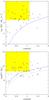 |
Fig. 1 Galaxy stellar mass (bottom) and SFR (top) for LGRB host galaxies considered in this paper. The lines indicate the limits shown in the figures of Savaglio et al. (2009): The solid and dashed lines in the bottom panel show the stellar mass as a function of redshift of a galaxy with a K-band magnitude of 24.3 and either an old stellar population or constant SFR, respectively. In the top panel, the line represents an Hα or [O II] emission flux of 1.3 × 10⁻¹⁷ erg s-1 or 0.7 × 10⁻¹⁷ erg s-1, respectively, assuming a dust extinction in the visual band A(V) = 0.53. The shaded area indicates our selection criteria: We work at redshift lower than 1.1 and above a minimal value for the stellar masses and SFR, so that our sample is complete. |
2.3. Relationships among galactic properties
The methods described in Sects. 2.1 and 2.2 provide constraints on the variation of the LGRB bias b on the SFR or on the galaxies stellar mass. However, this a dependence does not necessary imply a physical relationship. Indeed, these quantities may themselves be correlated to more fundamental ones for the physics of LGRBs (such as the metallicity). Important relations that we will use to analyse our results are:
-
The stellar mass – SFR relationship. The existence of a stel-lar mass – SFR relationship at all redshifts may be debated,but several studies indicate a good relation between the twoquantities at redshifts lower than about 1 from at least a sta-tistical point of view despite some dispersion (Brinchmannet al. 2004; Buatet al. 2008; Gilbanket al. 2011; Salmiet al. 2012; Bertaet al. 2013). This relation is nec-essary to use the method described in Sect. 2.2.Moreover, it can be used to attempt to determine trends with theSSFR by combining it with our results (b – stellar mass and b – SFR relationships). In practice, we will use the stellar mass – SFR relationship of the models of Boissier et al. (2010) in broad agreement with the observed trends in the redshift range of 0–1.1. We refer the reader to Sect. 5 for a discussion, including the role of the dispersion in this relation.
-
The stellar mass – SFR – metallicity relationship. Mannucci et al. (2010) found a fundamental metallicity relation (FMR) between the metallicity and a combination of the stellar mass and the SFR (see also Lara-López et al. 2010, for a similar relationship). This relation presents a smaller scatter than traditional mass-metallicity relationships and has the advantage of being independent of redshift (at least at redshift lower than 2.5). Moreover, the relation also holds for GRB hosts (Mannucci et al. 2011). Once a trend between b and the SFR (or b and the stellar mass) is established, we can use the stellar-mass SFR relationship to compute the stellar mass from the SFR (or vice-versa) and thus find a trend between b and the metallicity by simply assuming the Mannucci et al. (2010) relation.
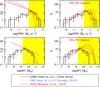 |
Fig. 2 Histograms of the stellar mass function (bottom) and SFR distribution (top) of the LGRB host galaxies. The shaded area indicates the region where we expect to be complete. Outside of this region, our results are likely to underestimate the number of host galaxies. In the bottom panels, the dotted histogram reports the stellar mass function of LGRB hosts by Savaglio (2012) as a comparison. In left panels, the LGRB host distributions are compared with those of star-forming galaxies as modelled in Boissier et al. (2010). Solid and dashed curve refers to redshift 0 and 1.1, respectively, while dotted lines are for intermediate redshifts (0.3, 0.5, 0.7, and 0.9). As the LGRB rate is proportional to the SFR (for constant b), a direct comparison between LGRB host and SFG distributions is not possible. Right panels show the same comparison when SFG distributions are weighted by the SFR. In this case, the LGRB host and SFG distribution should be identical for a constant bias b. |
3. LGRB hosts sample
3.1. Selection
To apply the methods described in Sect. 2, we need to know the distribution of stellar masses and SFRs of LGRB host galaxies. For this first application of the method, we try to determine these functions from the data available in the GHostS database (as on the 9th of July 2012). Figure 1 shows the SFR and stellar masses (as taken from the GHostS database) of the LGRB hosts as a function of redshift. The separation between short and long LGRBs is not uniquely defined (e.g. Zhang et al. 2012). For the present work, we removed all the bursts considered as short by Kopač et al. (2012) and the bursts with a duration shorter than 2 s. We limit our study to redshift lower than 1.1 where the Boissier et al. (2010) models used in our analysis represent a good description of the SFG population. Since the database is a compilation of all hosts known with public information, there is unfortunately not a clear limit on the stellar mass or SFR to adopt. However, the stellar masses derived from the hosts’ SED in Savaglio et al. (2009) which provide a high number of the data in the GHostS database, correlate well with the K band magnitude. The K band limit shown in Fig. 1 provides a good idea of the minimal stellar mass that can be measured as a function of redshift. Similarly, SFR are derived from a variety of SFR tracers, but the curve in Fig. 1 taken again from Savaglio et al. (2009) provides a good idea of the measurement limit in SFR. The SFRs from Savaglio et al. (2009) are corrected for dust attenuation using adequate extinction tracers, when they are available, or the average value of 0.5 magnitude when they are not. Based on our redshift range (z < 1.1) and these limits, we obtain an usable dynamical range by including galaxies with log (M ∗ /M⊙) > 9.25 for the study based on the mass (the same limit adopted in Savaglio 2012). Independently we construct a sample of galaxies with log (SFR/1 M⊙ yr-1) > 0.25 (i.e., SFR larger than about 1.8 M⊙ yr-1) for the study based on the SFR. This limit is conservative, compensating for the large uncertainties in SFR measurements. Of the 66 galaxies with measured stellar masses in GHostS, 35 LGRB hosts are found with z < 1.1 (20 above our stellar mass limit). Of the 48 galaxies with measured SFR in GHostS, 34 LGRB hosts are found with z < 1.1 (21 above our SFR limit).
3.2. Stellar mass and SFR distributions
The histograms of the measured stellar masses and SFR in LGRB hosts within our selection limits are shown in Fig. 2 (as a check, we randomly split our sample in two halves and obtained consistent distributions). In this figure, a turnover is observed below our selection limit: what shows indeed is that we are missing LGRB hosts below this limit. In the rest of the paper, we will then keep only the three bins for the largest values of the SFR and the stellar masses, for which we believe to be complete. The distribution of stellar masses and SFR in SFGs (from the models of Boissier et al. 2010) are also shown. A direct comparison between hosts and SFG distribution is not possible. Indeed hosts should present larger SFR than SFGs, even in absence of bias (constant b), since the LGRB rate is proportional to the SFR. As shown by Eq. (6), the bias b is proportional to the ratio of the two functions divided by the SFR. To obtain a meaningful comparison, we also show the SFR distribution of SFGs weighted by their SFR in the top-right panel of Fig. 2. In the absence of bias, the SFR weighted distribution for SFGs, and the LGRB hosts distribution should be identical. A similar effect applies to the stellar mass functions. We show in the bottom-right panel the stellar mass function of SFGs weighted by their SFR. In the bottom panel, we compare our stellar mass distribution with the stellar mass function of Savaglio (2012) for GRB hosts at redshift lower than 1.5. Despite the slightly different selections, the mass functions are consistent with each other within the statistical uncertainties. The main difference is found for the largest stellar masses. As a test, we added in our analysis a bin centred on 1011M⊙, including two fake hosts. With this bin, our distribution would be in perfect agreement with the Savaglio (2012) mass function. Except for this new bin, the results presented in the rest of the paper would be, of course, unchanged. The only difference would then be the addition of one extra point corresponding to 1011M⊙ for which we would obtain values of b similar to the one at 1010.5M⊙ with large error bars (due to the low number statistics), which agree with the overall trends found in the paper. In other words, the difference between our distribution and that of Savaglio (2012) could easily be explained by the absence of two bursts due to Poison noise. Adding them artificially leaves our conclusions unchanged.
The binning was chosen to have at least 10 LGRBs in the bin with the highest number of objects and to have a few objects in higher stellar masses and SFR bins. Above our completeness limits, we can consider the histograms as the true LGRB host mass function and SFR distribution (except for the normalisation, since we are interested only in relative trends). This is very different from the usual way to determine these functions from galaxy surveys for which galaxies of a given luminosity are detected only in a limited volume, and volume corrections have to be applied. In our case, the inclusion of the galaxy in our sample is not dependent on its luminosity or on the volume probed (as soon as it is possible to measure the SFR or the stellar mass). Indeed the selection is made by the detection and correct localisation of a LGRB so that it does not depend on its distance or on its host luminosity (excluding only dark bursts which are discussed in the next section). Then, the hosts are looked for and studied independently of their redshift. We avoid volume corrections by selecting a part of the space parameter (redshift, stellar mass, or SFR) where the SFR and stellar masses are sufficiently large for a measurement to be possible even at the largest redshift used.
3.3. Dark bursts
The functions obtained in the previous section could suffer from an observational bias. They are constructed only for host galaxies that were observed. The hosts of dark bursts with no optical afterglows, representing a maximum of the 30% of the LGRBs (e.g. Melandri et al. 2012) are usually not identified and may be absent from our sample. There are actually several definitions for dark bursts (e.g., Greiner et al. 2011), and many LGRB hosts are found from their X-ray afterglow, even without optical afterglow (e.g. Hjorth et al. 2012), so that the fraction missing from our sample is hard to determine but probably lower than the number quoted above. Melandri et al. (2012) found a similar redshift distribution between dark bursts and the general population of LGRBs, suggesting that our low redshift sample is also affected by dark bursts (even if their redshift distribution at redshifts lower than 1 is constrained by only very few objects).
It has been suggested that most of dark bursts are due to a high amount of dust extinction in the proximity of the LGRB, making it too faint to be observed (Melandri et al. 2012; Rossi et al. 2012). If dark bursts are indeed due to dust attenuation, it is expected that their relative number would vary with the SFR and stellar mass of their host galaxies. Indeed, Perley et al. (2013) and Krühler et al. (2011) found that the host galaxies of very dust-attenuated LGRBs show higher SFR and are more massive (again, few of their bursts are at redshifts lower than 1; thus, it is not completely obvious if this applies for the nearest hosts). On the other hand, Michałowski et al. (2012) found recently that an optically unbiased sample of host galaxies at redshift lower than 1 has a globally similar SFR and an amount of attenuation as normal galaxies.
As a summary, an increasing fraction of LGRB hosts with larger stellar mass and SFR may be missing from our sample, even if the situation is not completely clear. Our results could then not result exclusively from a real physical variation in b with various parameters but rather it quantifies how the dark burst bias depends on physical quantities in usual samples of hosts. The recent study of dark bursts hosts by Perley et al. (2013) still suggests that a physical dependence is needed.
4. Application in the redshift range 0–1.1
4.1. Bias – SFR and bias – stellar mass relationships
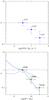 |
Fig. 3 Variation of the bias b with the stellar mass (bottom) and the SFR (top) with an arbitrary normalisation. The triangles show our results after interpolating the SFGs properties at the median redshift of the bin (indicated next to each symbols). In the bottom panel, the dashed lines indicate the results adopting the two regression lines of the stellar mass-SFR relation found in host galaxies (shown in Fig. 5) as explained in Sect. 5. The vertical error-bars indicates the statistical uncertainty on the number of LGRBs ( |

With the stellar masses and SFR distributions of both SFGs and LGRB hosts (shown in Fig. 2) it is easy to derive how the bias b depends on the SFR and stellar mass. Following Eqs. (6) and (7), the first step is to divide the distribution corresponding to host galaxies by the one corresponding to SFGs. For the stellar mass function, this can directly be done (since the mass function is constant in the redshift range). The SFR distribution of SFGs on the other hand depends on the redshift (as can be seen in Fig. 2). It was thus interpolated to the median redshift of the bin before performing the division in each SFR bin.
The next step consists of dividing by the SFR. For the method based on the stellar mass function, we have to adopt a stellar mass – SFR relationship that will give us the SFR for each stellar mass bin. This relation for SFGs evolves with redshift, according to the models in Boissier et al. (2010). Here again, we interpolate in each stellar mass bin to find the corresponding SFR for the median redshift of the bin.
Figure 3 shows the obtained relation between b and the stellar mass (bottom panel) and the SFR (top panel). While indication about the existence of a bias in the LGRB host population has been inferred from their properties (blue colors, low metallicities, etc.), our method allows us for the first time to quantify its dependence with SFR and stellar mass.
A similar trend as the one presented in Fig. 3 between the bias and the stellar mass is found by adopting the models at any fixed redshift between 0 an 1 rather than the median redshift in the bin. This indicates that the redshift distribution in each bin does not strongly influence our results. We tried different binning schemes for the stellar mass histogram (larger/narrower, and shifted by a factor 1.5), and a similar trend was always found.
The trend between the bias and the SFR is less robust, as the redshift evolution of the SFGs’ SFR distribution introduce a strong dispersion in our results, especially since our results are sensitive to the particular redshifts of the LGRBs in each bin. We should also note that the point in the highest redshift bin is poorly constrained: there is only one LGRB in this SFR bin and the SFGs SFR distribution for this high SFR may be under estimated (see Sect. 2.1), so that b is over estimated. As a result of these effects, the trend with the SFR slightly depends on the binning scheme. In most cases, a decrease in b with the SFR is still suggested, but the relation is weaker for large bins (1 dex).
Combining the trends found between b and the stellar mass (or with the SFR) and the stellar mass-SFR relationship, it is straightforward to derive how b depends on the SSFR. Several studies found that LGRB hosts tend to have larger SSFRs than field galaxies (e.g., Christensen et al. 2004; Castro Cerón et al. 2006). Surprisingly, we do not find a clear trend of b with the SSFR. However, the very narrow dynamical range of SSFR probed by our sample, which is less than 0.5 dex, and the uncertainties in the determination of both stellar mass and SFR prevent us to draw any conclusion about this issue.
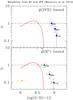 |
Fig. 4 Relation between b and the metallicity derived from the empirical FMR relationship of Mannucci et al. (2010). The vertical error bars correspond to the statistical uncertainty on the number of LGRBs. The horizontal error bar attached to each symbol corresponds to the width of the bin used at the beginning of the method. The horizontal bar in the bottom-left part of the figure indicates a systematic uncertainty on abundance measurements of a typical factor 2. The top panel shows the results based on the SFR distribution function, and the bottom panels the results based on the stellar mass functions. Finally, the curve indicates the fraction of SN Ic-WO supernovae (with which LGRBs could be associated), according to the models of Georgy et al. (2009). |
4.2. Bias as a function of metallicity
Combining the trends found between b and the stellar mass (i.e., with the method based on the stellar mass function) and the stellar mass-SFR relation interpolated at the median redshift of each bin, we can obtain a list of (b, stellar mass, and SFR) triplets. Another set of triplets can be obtained starting from the trend between b and the SFR (i.e., the method based on the SFR distribution). The FMR of Mannucci et al. (2010) then allows us to compute the metallicity of the galaxy from the SFR and stellar mass in each of these triplets.
The relations between b and the metallicity obtained in this way are shown on Fig. 4. When we start from the b-stellar mass relationship, a clear trend with metallicity is obtained. It is also suggested starting from the b-SFR relationship, but the uncertainties are larger and the dynamical range more narrow.
These trends are compared to the predictions of Georgy et al. (2009) for SN Ic-WO (SN Ic with progenitors consisting of Wolf-Rayet stars with carbon surface abundance that is superior to nitrogen abundance and with a C+O to He ratio in number larger than 1). Georgy et al. (2009) suggests a fraction of these SN could give rise to LGRBs. They predict a rate that is a function of the metallicity and is shown as the curve in Fig. 4 (with an arbitrary normalisation). In the case of their model, the metallicity is not measured but a physical parameter. Thus, the comparison suffers from the large uncertainties in the calibration of metallicity indicators (e.g. Kewley & Ellison 2008). In the figure, we indicate a typical 0.15 dex uncertainty that corresponds to a factor 2 total variation for illustrative purposes. In relative terms, the drop with metallicity found by Georgy et al. (2009) is slightly stronger than the trend found in our method based on the stellar mass (the method that is better constrained). On the absolute scale, we find the decrease in b at a much higher metallicity than found by Georgy et al. (2009), but we remind the reader that our determination of the metallicity is based on the FMR relation that is dispersed. If LGRBs prefer low metallicity, they will be found at the low metallicity end of the scatter. Full models considering the scatter in SFGs could help us to test this possibility but are beyond the scope of the simple approach proposed in this paper.
Our progressive decrease in the bias is at odds with the the idea of a simple metallicity cut-off at a metallicity ten times lower than solar, as proposed e.g. by Niino et al. (2009) on the basis of the Lyα emission of LGRB host galaxies statistics. This trend agrees with the analysis of Campisi et al. (2011), who found no need for a low-metallicity threshold (see also Levesque et al. 2010b; Graham & Fruchter 2013). These comparisons illustrate that our method already provides a quantification of the bias-metallicity relationship that can be compared to other recent theoretical or empirical works. Nevertheless, our results will have to be confirmed with higher statistics and better defined samples in the future.
5. Discussion: on the enhanced SFR in LGRB hosts
The relation between the SFR and the stellar mass observed in LGRBs differs from the one observed in SFGs, since LGRB host galaxies have higher SSFR (Christensen et al. 2004; Castro Cerón et al. 2006). While we argued that SFGs should be the parent population of galaxies providing host galaxies, we cannot reproduce the stellar mass-SFR relationship of LGRBs with the models of normal SFGs. This can be seen even in our sample in Fig. 5, where the Boissier et al. (2010) models are found below LGRB hosts. This figure may seem a bit different from the picture emerging from Fig. 12 of Savaglio et al. (2009) in which the stellar mass-SFR relation of a sample of GRB hosts seems similar to the one observed in samples of massive star-forming galaxies and Lyman-break galaxies at high redshift. The differences between their result and our study are: i) the selection of high-redshift typical galaxies (e.g. Lyman-break galaxies) may lead to a sample not representing the underlying star-forming population as a whole (bias towards active galaxies); ii) our study is limited to redshift lower than 1.1, where less extreme objects in terms of SFR are usually found; and iii) the models represent typical star-forming galaxies but may miss the more active ones (see Sect. 2.1).
This last point is related to the models that have smooth star formation histories without any dispersion in the SFR at a given stellar mass. On the contrary, galaxies may suffer episodical increases of their SFR (associated with e.g. interactions or mergers) during their evolution, that would bring them above the underlying stellar mass – SFR relationship (thus creating dispersion in this relation). Because LGRBs are related to massive stars, LGRB host galaxies are more likely to be found among these starbursts (even if b is constant), which is a simple way to explain the enhanced SSFR in LGRB host galaxies. In other words, LGRB hosts will be preferentially found at the upper end of the SSFR distribution as galaxies present a scatter of SSFR, even if the SSFR by itself has no influence on the occurrence of a burst. A drawback of our method is that such a dispersion is not considered in the models of SFGs. However, the general effect would be simply a shift in the stellar-mass – SFR relationship towards larger SFR during the events, which could produce the systematic shift between SFGs and host galaxies observed in Fig. 5, if variations of the SFR history affect all galaxies independently of their stellar mass. We actually tested how much our results could be affected by the evidence that we relied on the stellar mass-SFR relation of SFGs, which is lower than the one observed in host galaxies. To this aim, we fit the relation found in LGRBs (the two regression lines are shown in Fig. 5). In Fig. 3, we then added the b-stellar mass relations obtained by adopting these fits of the stellar mass-SFR relation in LGRB host galaxies (but without any information concerning its redshift evolution) rather than the one from SFGs: the two dashed lines in Fig. 3 correspond to the two regression lines in Fig. 5. Indeed, we obtain trends consistent with the one found with the SFGs’ stellar mass-SFR relationship. The decrease in b with the stellar mass above 109M⊙ is a robust result, despite this difficulty.
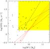 |
Fig. 5 Stellar mass-SFR relation of LGRB hosts (symbols) compared to that taken from the models of Boissier et al. (2010) for SFGs shown as a set of curves (solid at redshift 0, dashed at redshift 1.1, dotted for intermediate redshifts). The shaded area corresponds to our completeness limits. The dashed lines within this area are the two regression lines (for the SFR as a function of the stellar mass and the stellar mass as a function of the SFR) computed from the LGRB hosts data. |
Recent simulations show that interactions and mergers may indeed temporarily increase the star formation efficiency (by up to a factor 10 according to Teyssier et al. 2010). Simulations also indicate that low metallicity gas may be brought towards the inner part of galaxies diluting its metallicity during interactions (e.g. Montuori et al. 2010; Rupke et al. 2010; Perez et al. 2011). There are observational indications of reduced metallicities in merging pairs (Kewley et al. 2006; Michel-Dansac et al. 2008) or of galaxies with elevated merger-induced star formation (Rupke et al. 2008). Montuori et al. (2010) show examples of their models in their Fig. 1, where a large increase in the gas in the inner galaxy leads to a large SFR increase (by a factor up to 10) and a simultaneous dilution of the metallicity (from 0.1 to 0.3 dex). The metals produced in stars created during this peak of star formation will enrich the gas and future generation of stars, but the stars themselves created during the event have a diluted metallicity. This simultaneous increase in the SFR and decrease in the metallicity would make the galaxy stay at approximately the same spot in the FMR relation of Mannucci et al. (2010): for a 1010M⊙ galaxy with a SFR going from 1 to 10 M⊙ yr-1, the metallicity given by the fit from Mannucci et al. (2010) would decrease from 8.9 to 8.75, which is a similar change to the metal dilution found in the models. While it would be difficult to consider all the possible interactions in our approach, these increased SFR (favouring LGRBs in numbers) and dilution of the metallicity would simply explain the tendency for host galaxies to be shifted with respect to normal galaxies towards lower metallicities and higher SFR (see also Kocevski & West 2011). If this happens for galaxies of all masses (or all SFR before the interaction) in a similar manner, the effect would be systematic, and thus it would not erase possible trends of b with galactic properties little affected by this event, such as the stellar mass. In this case, our simple method should indeed provide correct results, even if these events are not (yet) included in the models we used.
In the future, we will include scatter in the models of the evolution of star-forming galaxies (due to interactions, mergers, and environment) to see if the trends found with the simple method are still recovered with the simultaneous enhancement of the SSFR and the reduction of metallicity in host galaxies.
6. Conclusion
The main objective of this paper was to present a simple empirical method to measure how the bias b (the ratio between the LGRB rate per galaxy and the SFR) may depend on physical quantities characterising the host galaxies (and thus the environment of the exploding massive star).
The method is based on comparing the stellar mass function and SFR distribution of LGRB host galaxies to those of star-forming galaxies, which are the expected parent population of LGRBs. For simplicity, we adopt the simple simple model of Boissier et al. (2010) for this family. We work within a redshift range (and a parameter space) where all quantities are well known. We also take advantage known relationships exhibited by the the star-forming galaxies to easily link various parameters (stellar masses, SFR, and metallicity). Given the statistics of LGRB events, a wide redshift range has to be considered, while some properties of galaxies evolve during the corresponding time interval. Within the redshift range where the relations are known, it is still possible to interpolate to the median redshift of the data to partially eliminate this problem.
When applied to a current sample of LGRBs at redshifts lower than 1.1 with host galaxies of stellar masses higher than 109.25M⊙ and SFR higher than 1.8 M⊙ yr-1, the method allows us to obtain the variation of the bias b with the stellar mass and SFR. We obtain a strong trend of decreasing b with the stellar mass of the host galaxies (Fig. 3). This result is robust even if the models used for star-forming galaxies do not include the scatter that would create interactions and starbursts that may occur during the evolution of galaxies. These events may be responsible for the enhanced SFR and dilluted metallicity in LGRB hosts, as discussed in Sect. 5. A similar trend is found with the SFR. However, the uncertainties are larger in this case: contrary to the stellar mass function, the SFR distribution evolves with redshift and suffers larger uncertainties. We do not find any trend between b and the SSFR (LGRBs are found in galaxies with higher SSFR, but b does not depend on it), although our dynamical range is too narrow to obtain a definitive answer.
The trends found between the bias b and the stellar mass or the SFR do not demonstrate a physical influence of these parameters on the occurrence of LGRBs since these are unknown to massive stars that may explode as LGRBs. The properties of SFGs allow us to indirectly relate them to the metallicity that is likely to play an important role in the final stages of stellar evolution and thus on the occurrence of LGRBs. We obtain a clear trend of decreasing bias with increasing metallicity (Fig. 4) that can put constraints on the physics of LGRB progenitors. Part of the relation that we obtained between the bias b and the stellar mass, the SFR, and the metallicity could also be due to dark bursts that are missed in usual studies of LGRB host galaxies. A better determination of the properties of dark burst hosts in the same redshift range as our study could help to distinguish between the intrinsic trend of b with the metallicity or the existence of an observational bias (massive, metal-rich galaxies missing from our samples).
In summary, this first application of our method suggests a clear trend of decreasing bias b with increasing metallicity despite large uncertainties and low statistics, that may constrain the models of LGRB progenitors (role of metallicity in stellar evolution) or their environment (dust attenuation). We are confident that this method will become much more powerful in the future, since i) the problem of dark bursts will be alleviated by robotic telescopes operating in the near IR; ii) larger samples of LGRB host galaxies detected below redshift unity will be characterised, allowing us to use better controlled samples and split the data into narrower redshift intervals, which limits the evolutionary effects; and iii) it will also be possible to extend the method to higher redshifts with the determination of stellar mass functions and properties of SFGs in the early universe
Short duration gamma-ray bursts (usually lasting less than 2 s) are not associated with massive stars and star formation; they are not considered in this work.
Acknowledgments
This research has made use of the GHostS database (http://www.GRBhosts.org), which is partly funded by Spitzer/NASA grant RSA Agreement No. 1287913. It was performed in the context and with the support of the CNRS GDRE “Exploring the Dawn of the Universe with the GRBs” (http://lamwws.oamp.fr/gdre/GdreGRBs). We thank the anonymous referee for constructive comments. S.B. thanks the organisers of the “Chemical evolution of GRB host galaxies” Sesto workshop (F. Matteucci and F. Longo), of the 5th GDRE workshop in IAP, and the participants to these events. The suggestions made by the participants helped to improve this work. S.B. thanks everybody at the Trieste Observatory for welcoming him for several periods during which part of this work was performed and finally for discussion related to this work: O. Cucciati, S. Heinis, and O. Ilbert.
References
- Arnouts, S., Walcher, C. J., Le Fèvre, O., et al. 2007, A&A, 476, 137 [NASA ADS] [CrossRef] [EDP Sciences] [Google Scholar]
- Basa, S., Cuby, J. G., Savaglio, S., et al. 2012, A&A, 542, A103 [NASA ADS] [CrossRef] [EDP Sciences] [Google Scholar]
- Bell, E. F., Zheng, X. Z., Papovich, C., et al. 2007, ApJ, 663, 834 [NASA ADS] [CrossRef] [Google Scholar]
- Berta, S., Lutz, D., Santini, P., et al. 2013, A&A, 551, A100 [NASA ADS] [CrossRef] [EDP Sciences] [Google Scholar]
- Bloom, J. S., Djorgovski, S. G., Kulkarni, S. R., & Frail, D. A. 1998, ApJ, 507, L25 [NASA ADS] [CrossRef] [Google Scholar]
- Boissier, S., Buat, V., & Ilbert, O. 2010, A&A, 522, A18 [NASA ADS] [CrossRef] [EDP Sciences] [Google Scholar]
- Borch, A., Meisenheimer, K., Bell, E. F., et al. 2006, A&A, 453, 869 [NASA ADS] [CrossRef] [EDP Sciences] [Google Scholar]
- Bothwell, M. S., Kenicutt, R. C., Johnson, B. D., et al. 2011, MNRAS, 415, 1815 [NASA ADS] [CrossRef] [Google Scholar]
- Brinchmann, J., Charlot, S., White, S. D. M., et al. 2004, MNRAS, 351, 1151 [NASA ADS] [CrossRef] [Google Scholar]
- Buat, V., Boissier, S., Burgarella, D., et al. 2008, A&A, 483, 107 [NASA ADS] [CrossRef] [EDP Sciences] [Google Scholar]
- Campisi, M. A., Tapparello, C., Salvaterra, R., Mannucci, F., & Colpi, M. 2011, MNRAS, 417, 1013 [CrossRef] [Google Scholar]
- Castro Cerón, J. M., Michałowski, M. J., Hjorth, J., et al. 2006, ApJ, 653, L85 [NASA ADS] [CrossRef] [Google Scholar]
- Castro Cerón, J. M., Michałowski, M. J., Hjorth, J., et al. 2010, ApJ, 721, 1919 [NASA ADS] [CrossRef] [Google Scholar]
- Christensen, L., Hjorth, J., & Gorosabel, J. 2004, A&A, 425, 913 [NASA ADS] [CrossRef] [EDP Sciences] [Google Scholar]
- Cowie, L. L., & Barger, A. J. 2008, ApJ, 686, 72 [NASA ADS] [CrossRef] [Google Scholar]
- Daigne, F., Rossi, E. M., & Mochkovitch, R. 2006, MNRAS, 372, 1034 [NASA ADS] [CrossRef] [Google Scholar]
- Elliott, J., Greiner, J., Khochfar, S., et al. 2012, A&A, 539, A113 [NASA ADS] [CrossRef] [EDP Sciences] [Google Scholar]
- Fruchter, A. S., Thorsett, S. E., Metzger, M. R., et al. 1999, ApJ, 519, L13 [NASA ADS] [CrossRef] [Google Scholar]
- Fruchter, A. S., Levan, A. J., Strolger, L., et al. 2006, Nature, 441, 463 [NASA ADS] [CrossRef] [PubMed] [Google Scholar]
- Georgy, C., Meynet, G., Walder, R., Folini, D., & Maeder, A. 2009, A&A, 502, 611 [NASA ADS] [CrossRef] [EDP Sciences] [Google Scholar]
- Gilbank, D. G., Bower, R. G., Glazebrook, K., et al. 2011, MNRAS, 414, 304 [NASA ADS] [CrossRef] [Google Scholar]
- Graham, J. F., & Fruchter, A. S. 2013, EAS Publ. Ser., 61, 413 [CrossRef] [Google Scholar]
- Greiner, J., Krühler, T., Klose, S., et al. 2011, A&A, 526, A30 [NASA ADS] [CrossRef] [EDP Sciences] [Google Scholar]
- Han, X. H., Hammer, F., Liang, Y. C., et al. 2010, A&A, 514, A24 [NASA ADS] [CrossRef] [EDP Sciences] [Google Scholar]
- Hjorth, J., Malesani, D., Jakobsson, P., et al. 2012, ApJ, 756, 187 [NASA ADS] [CrossRef] [Google Scholar]
- Ilbert, O., Salvato, M., Le Floc’h, E., et al. 2010, ApJ, 709, 644 [NASA ADS] [CrossRef] [Google Scholar]
- Ilbert, O., McCracken, H. J., Le Fevre, O., et al. 2013, A&A, 556, A55 [NASA ADS] [CrossRef] [EDP Sciences] [Google Scholar]
- Kewley, L. J., & Ellison, S. L. 2008, ApJ, 681, 1183 [NASA ADS] [CrossRef] [Google Scholar]
- Kewley, L. J., Geller, M. J., & Barton, E. J. 2006, AJ, 131, 2004 [NASA ADS] [CrossRef] [Google Scholar]
- Kistler, M. D., Yüksel, H., Beacom, J. F., Hopkins, A. M., & Wyithe, J. S. B. 2009, ApJ, 705, L104 [NASA ADS] [CrossRef] [Google Scholar]
- Kocevski, D., & West, A. A. 2011, ApJ, 735, L8 [NASA ADS] [CrossRef] [Google Scholar]
- Kocevski, D., West, A. A., & Modjaz, M. 2009, ApJ, 702, 377 [NASA ADS] [CrossRef] [Google Scholar]
- Kopač, D., D’Avanzo, P., Melandri, A., et al. 2012, MNRAS, 424, 2392 [NASA ADS] [CrossRef] [Google Scholar]
- Krühler, T., Greiner, J., Schady, P., et al. 2011, A&A, 534, A108 [NASA ADS] [CrossRef] [EDP Sciences] [Google Scholar]
- Lara-López, M. A., Cepa, J., Bongiovanni, A., et al. 2010, A&A, 521, L53 [NASA ADS] [CrossRef] [EDP Sciences] [Google Scholar]
- Le Floc’h, E., Duc, P.-A., Mirabel, I. F., et al. 2003, A&A, 400, 499 [NASA ADS] [CrossRef] [EDP Sciences] [Google Scholar]
- Le Floc’h, E., Papovich, C., Dole, H., et al. 2005, ApJ, 632, 169 [NASA ADS] [CrossRef] [Google Scholar]
- Levesque, E. M., Kewley, L. J., Berger, E., & Zahid, H. J. 2010a, AJ, 140, 1557 [NASA ADS] [CrossRef] [Google Scholar]
- Levesque, E. M., Kewley, L. J., Graham, J. F., & Fruchter, A. S. 2010b, ApJ, 712, L26 [NASA ADS] [CrossRef] [Google Scholar]
- MacFadyen, A. I., & Woosley, S. E. 1999, ApJ, 524, 262 [NASA ADS] [CrossRef] [Google Scholar]
- Magnelli, B., Elbaz, D., Chary, R. R., et al. 2009, A&A, 496, 57 [NASA ADS] [CrossRef] [EDP Sciences] [Google Scholar]
- Mannucci, F., Cresci, G., Maiolino, R., Marconi, A., & Gnerucci, A. 2010, MNRAS, 408, 2115 [NASA ADS] [CrossRef] [Google Scholar]
- Mannucci, F., Salvaterra, R., & Campisi, M. A. 2011, MNRAS, 414, 1263 [NASA ADS] [CrossRef] [Google Scholar]
- Martin, D. C., Seibert, M., Buat, V., et al. 2005, ApJ, 619, L59 [NASA ADS] [CrossRef] [Google Scholar]
- Melandri, A., Sbarufatti, B., D’Avanzo, P., et al. 2012, MNRAS, 421, 1265 [NASA ADS] [CrossRef] [Google Scholar]
- Michałowski, M. J., Kamble, A., Hjorth, J., et al. 2012, ApJ, 755, 85 [NASA ADS] [CrossRef] [Google Scholar]
- Michel-Dansac, L., Lambas, D. G., Alonso, M. S., & Tissera, P. 2008, MNRAS, 386, L82 [NASA ADS] [CrossRef] [Google Scholar]
- Modjaz, M., Kewley, L., Kirshner, R. P., et al. 2008, AJ, 135, 1136 [NASA ADS] [CrossRef] [Google Scholar]
- Montuori, M., Di Matteo, P., Lehnert, M. D., Combes, F., & Semelin, B. 2010, A&A, 518, A56 [NASA ADS] [CrossRef] [EDP Sciences] [Google Scholar]
- Niino, Y., Totani, T., & Kobayashi, M. A. R. 2009, ApJ, 707, 1634 [NASA ADS] [CrossRef] [Google Scholar]
- Perez, J., Michel-Dansac, L., & Tissera, P. B. 2011, MNRAS, 417, 580 [NASA ADS] [CrossRef] [Google Scholar]
- Perley, D. A., Levan, A. J., Tanvir, N. R., et al. 2013, ApJ, submitted [arXiv:1301.5903] [Google Scholar]
- Podsiadlowski, P., Ivanova, N., Justham, S., & Rappaport, S. 2010, MNRAS, 406, 840 [NASA ADS] [Google Scholar]
- Pozzetti, L., Bolzonella, M., Zucca, E., et al. 2010, A&A, 523, A13 [NASA ADS] [CrossRef] [EDP Sciences] [Google Scholar]
- Qin, S.-F., Liang, E.-W., Lu, R.-J., Wei, J.-Y., & Zhang, S.-N. 2010, MNRAS, 406, 558 [NASA ADS] [CrossRef] [Google Scholar]
- Robertson, B. E., & Ellis, R. S. 2012, ApJ, 744, 95 [NASA ADS] [CrossRef] [Google Scholar]
- Rodighiero, G., Vaccari, M., Franceschini, A., et al. 2010, A&A, 515, A8 [NASA ADS] [CrossRef] [EDP Sciences] [Google Scholar]
- Rossi, A., Klose, S., Ferrero, P., et al. 2012, A&A, 545, A77 [Google Scholar]
- Rupke, D. S. N., Veilleux, S., & Baker, A. J. 2008, ApJ, 674, 172 [NASA ADS] [CrossRef] [Google Scholar]
- Rupke, D. S. N., Kewley, L. J., & Barnes, J. E. 2010, ApJ, 710, L156 [NASA ADS] [CrossRef] [Google Scholar]
- Salmi, F., Daddi, E., Elbaz, D., et al. 2012, ApJ, 754, L14 [NASA ADS] [CrossRef] [Google Scholar]
- Salvaterra, R., Campana, S., Vergani, S. D., et al. 2012, ApJ, 749, 68 [NASA ADS] [CrossRef] [Google Scholar]
- Savaglio, S. 2012, Astron. Nachr., 333, 480 [Google Scholar]
- Savaglio, S., Glazebrook, K., & Le Borgne, D. 2009, ApJ, 691, 182 [NASA ADS] [CrossRef] [MathSciNet] [Google Scholar]
- Teyssier, R., Chapon, D., & Bournaud, F. 2010, ApJ, 720, L149 [NASA ADS] [CrossRef] [Google Scholar]
- Vergani, D., Scodeggio, M., Pozzetti, L., et al. 2008, A&A, 487, 89 [NASA ADS] [CrossRef] [EDP Sciences] [Google Scholar]
- Virgili, F. J., Zhang, B., Nagamine, K., & Choi, J.-H. 2011, MNRAS, 417, 3025 [NASA ADS] [CrossRef] [Google Scholar]
- Wolf, C., & Podsiadlowski, P. 2007, MNRAS, 375, 1049 [NASA ADS] [CrossRef] [Google Scholar]
- Woosley, S. E., & Bloom, J. S. 2006, ARA&A, 44, 507 [NASA ADS] [CrossRef] [Google Scholar]
- Woosley, S. E., & Heger, A. 2006, ApJ, 637, 914 [NASA ADS] [CrossRef] [Google Scholar]
- Zhang, F.-W., Shao, L., Yan, J.-Z., & Wei, D.-M. 2012, ApJ, 750, 88 [NASA ADS] [CrossRef] [Google Scholar]
All Figures
|
Fig. 1 Galaxy stellar mass (bottom) and SFR (top) for LGRB host galaxies considered in this paper. The lines indicate the limits shown in the figures of Savaglio et al. (2009): The solid and dashed lines in the bottom panel show the stellar mass as a function of redshift of a galaxy with a K-band magnitude of 24.3 and either an old stellar population or constant SFR, respectively. In the top panel, the line represents an Hα or [O II] emission flux of 1.3 × 10⁻¹⁷ erg s-1 or 0.7 × 10⁻¹⁷ erg s-1, respectively, assuming a dust extinction in the visual band A(V) = 0.53. The shaded area indicates our selection criteria: We work at redshift lower than 1.1 and above a minimal value for the stellar masses and SFR, so that our sample is complete. |
| In the text | |
|
Fig. 2 Histograms of the stellar mass function (bottom) and SFR distribution (top) of the LGRB host galaxies. The shaded area indicates the region where we expect to be complete. Outside of this region, our results are likely to underestimate the number of host galaxies. In the bottom panels, the dotted histogram reports the stellar mass function of LGRB hosts by Savaglio (2012) as a comparison. In left panels, the LGRB host distributions are compared with those of star-forming galaxies as modelled in Boissier et al. (2010). Solid and dashed curve refers to redshift 0 and 1.1, respectively, while dotted lines are for intermediate redshifts (0.3, 0.5, 0.7, and 0.9). As the LGRB rate is proportional to the SFR (for constant b), a direct comparison between LGRB host and SFG distributions is not possible. Right panels show the same comparison when SFG distributions are weighted by the SFR. In this case, the LGRB host and SFG distribution should be identical for a constant bias b. |
| In the text | |
|
Fig. 3 Variation of the bias b with the stellar mass (bottom) and the SFR (top) with an arbitrary normalisation. The triangles show our results after interpolating the SFGs properties at the median redshift of the bin (indicated next to each symbols). In the bottom panel, the dashed lines indicate the results adopting the two regression lines of the stellar mass-SFR relation found in host galaxies (shown in Fig. 5) as explained in Sect. 5. The vertical error-bars indicates the statistical uncertainty on the number of LGRBs ( |
| In the text | |
|
Fig. 4 Relation between b and the metallicity derived from the empirical FMR relationship of Mannucci et al. (2010). The vertical error bars correspond to the statistical uncertainty on the number of LGRBs. The horizontal error bar attached to each symbol corresponds to the width of the bin used at the beginning of the method. The horizontal bar in the bottom-left part of the figure indicates a systematic uncertainty on abundance measurements of a typical factor 2. The top panel shows the results based on the SFR distribution function, and the bottom panels the results based on the stellar mass functions. Finally, the curve indicates the fraction of SN Ic-WO supernovae (with which LGRBs could be associated), according to the models of Georgy et al. (2009). |
| In the text | |
|
Fig. 5 Stellar mass-SFR relation of LGRB hosts (symbols) compared to that taken from the models of Boissier et al. (2010) for SFGs shown as a set of curves (solid at redshift 0, dashed at redshift 1.1, dotted for intermediate redshifts). The shaded area corresponds to our completeness limits. The dashed lines within this area are the two regression lines (for the SFR as a function of the stellar mass and the stellar mass as a function of the SFR) computed from the LGRB hosts data. |
| In the text | |
Current usage metrics show cumulative count of Article Views (full-text article views including HTML views, PDF and ePub downloads, according to the available data) and Abstracts Views on Vision4Press platform.
Data correspond to usage on the plateform after 2015. The current usage metrics is available 48-96 hours after online publication and is updated daily on week days.
Initial download of the metrics may take a while.