| Issue |
A&A
Volume 556, August 2013
|
|
|---|---|---|
| Article Number | A89 | |
| Number of page(s) | 46 | |
| Section | Interstellar and circumstellar matter | |
| DOI | https://doi.org/10.1051/0004-6361/201220849 | |
| Published online | 02 August 2013 | |
High-J CO survey of low-mass protostars observed with Herschel-HIFI⋆,⋆⋆
1
Leiden Observatory, Leiden University,
PO Box 9513, 2300 RA
Leiden, The
Netherlands
e-mail:
This email address is being protected from spambots. You need JavaScript enabled to view it.
2
Harvard-Smithsonian Center for Astrophysics, 60 Garden
Street, Cambridge,
MA
02138,
USA
3
Max Planck Institut für Extraterrestrische Physik,
Giessenbachstrasse 1,
85748
Garching,
Germany
4
Observatorio Astronómico Nacional (IGN),
Calle Alfonso XII, 3,
28014
Madrid,
Spain
5
Observatorio Astronómico Nacional, Apartado 112, 28803
Alcalá de Henares,
Spain
6
Department of Astronomy, University of Michigan,
500 Church Street, Ann Arbor, MI
48109-1042,
USA
7
Niels Bohr Institute, University of Copenhagen,
Juliane Maries Vej 30,
2100
Copenhagen Ø.,
Denmark
8
Centre for Star and Planet Formation, Natural History Museum of
Denmark, University of Copenhagen, Øster Voldgade 5–7, 1350
Copenhagen K.,
Denmark
Received: 4 December 2012
Accepted: 14 June 2013
Abstract
Context. In the deeply embedded stage of star formation, protostars start to heat and disperse their surrounding cloud cores. The evolution of these sources has traditionally been traced through dust continuum spectral energy distributions (SEDs), but the use of CO excitation as an evolutionary probe has not yet been explored due to the lack of high-J CO observations.
Aims. The aim is to constrain the physical characteristics (excitation, kinematics, column density) of the warm gas in low-mass protostellar envelopes using spectrally resolved Herschel data of CO and compare those with the colder gas traced by lower excitation lines.
Methods. Herschel-HIFI observations of high-J lines of 12CO, 13CO, and C18O (up to Ju = 10, Eu up to 300 K) are presented toward 26 deeply embedded low-mass Class 0 and Class I young stellar objects, obtained as part of the Water In Star-forming regions with Herschel (WISH) key program. This is the first large spectrally resolved high-J CO survey conducted for these types of sources. Complementary lower J CO maps were observed using ground-based telescopes, such as the JCMT and APEX and convolved to matching beam sizes.
Results. The 12CO 10–9 line is detected for all objects and can generally be decomposed into a narrow and a broad component owing to the quiescent envelope and entrained outflow material, respectively. The 12CO excitation temperature increases with velocity from ~60 K up to ~130 K. The median excitation temperatures for 12CO, 13CO, and C18O derived from single-temperature fits to the Ju = 2–10 integrated intensities are ~70 K, 48 K and 37 K, respectively, with no significant difference between Class 0 and Class I sources and no trend with Menv or Lbol. Thus, in contrast to the continuum SEDs, the spectral line energy distributions (SLEDs) do not show any evolution during the embedded stage. In contrast, the integrated line intensities of all CO isotopologs show a clear decrease with evolutionary stage as the envelope is dispersed. Models of the collapse and evolution of protostellar envelopes reproduce the C18O results well, but underproduce the 13CO and 12CO excitation temperatures, due to lack of UV heating and outflow components in those models. The H2O 110 − 101/CO 10–9 intensity ratio does not change significantly with velocity, in contrast to the H2O/CO 3–2 ratio, indicating that CO 10–9 is the lowest transition for which the line wings probe the same warm shocked gas as H2O. Modeling of the full suite of C18O lines indicates an abundance profile for Class 0 sources that is consistent with a freeze-out zone below 25 K and evaporation at higher temperatures, but with some fraction of the CO transformed into other species in the cold phase. In contrast, the observations for two Class I sources in Ophiuchus are consistent with a constant high CO abundance profile.
Conclusions. The velocity resolved line profiles trace the evolution from the Class 0 to the Class I phase through decreasing line intensities, less prominent outflow wings, and increasing average CO abundances. However, the CO excitation temperature stays nearly constant. The multiple components found here indicate that the analysis of spectrally unresolved data, such as provided by SPIRE and PACS, must be done with caution.
Key words: astrochemistry / stars: formation / stars: protostars / ISM: molecules / techniques: spectroscopic
Herschel is an ESA space observatory with science instruments provided by European-led Principal Investigator consortia and with important participation from NASA.
Appendices C and D are available in electronic form at http://www.aanda.org
© ESO, 2013
1. Introduction
Low-mass stars like our Sun form deep inside collapsing molecular clouds by accreting material onto a central dense source. As the source evolves, gas and dust move from the envelope to the disk and onto the star, resulting in a decrease in the envelope mass and a shift in the peak of the continuum spectral energy distribution to shorter wavelengths (e.g., Lada 1999; André et al. 2000; Young & Evans 2005). At the same time, jets and winds from the protostar entrain material and disperse the envelope. Spectral lines at submillimeter wavelengths trace this dense molecular gas and reveal both the kinematic signature of collapse (Gregersen et al. 1997; Myers et al. 2000; Kristensen et al. 2012) as well as the high velocity gas in the outflows (Arce et al. 2007).
The most commonly used probe is CO because it is the second most abundant molecule after H2, has a simple energy level structure, and all main isotopolog lines are readily detectable (12CO, 13CO, C18O, C17O). Because of its small dipole moment, its rotational lines are easily excited and therefore provide an excellent estimate of the gas column density and the kinetic temperature. Although low excitation lines of CO have been observed in protostars for decades (e.g., Hayashi et al. 1994; Blake et al. 1995; Bontemps et al. 1996; Jørgensen et al. 2002; Fuller & Ladd 2002; Tachihara et al. 2002; Hatchell et al. 2005), no systematic studies have been undertaken so far of the higher excitation lines that probe the warm gas (T > 100 K) during protostellar evolution. Ground-based observations of other molecules exist as well and in some (but not all) show low-mass sources a variety of complex organic species commonly ascribed to “hot cores” where ices evaporate molecules back into the gas phase (e.g., van Dishoeck & Blake 1998; Ceccarelli et al. 2007). Quantifying these hot core abundunces has been complicated by the lack of a good reference of the H2 column density in this warm ≥100 K gas.
With the launch of the Herschel Space Observatory (Pilbratt et al. 2010) equipped with new efficient detectors, observations of low-mass protostars in higher-J transitions of CO have become possible. In this paper, high-J refers to the lines Ju ≥ 6 (Eu > 100 K) and low-J refers to Ju ≤ 5 (Eu < 100 K). The Heterodyne Instrument for Far-Infrared (HIFI; de Graauw et al. 2010) on Herschel offers a unique opportunity to observe spectrally resolved high-J CO lines of various isotopologs with unprecendented sensitivity (see Yıldız et al. 2010; Plume et al. 2012, for early results). Even higher transitions of CO up to Ju = 50 are now routinely observed with the Photoconducting Array and Spectrometer (PACS; Poglitsch et al. 2010) and the Spectral and Photometric Imaging Receiver (SPIRE; Griffin et al. 2010) instruments on Herschel, but those data are spectrally unresolved, detect mostly 12CO, and probe primarily a hot shocked gas component associated with the source (e.g., van Kempen et al. 2010; Herczeg et al. 2012; Goicoechea et al. 2012; Karska et al. 2013; Manoj et al. 2013; Green et al. 2013). To study the bulk of the protostellar system and disentangle the various physical components, velocity resolved lines of isotopologs including optically thin C18O are needed.
In this paper, we use Herschel-HIFI single pointing observations of high-J CO and its isotopologs up to the 10–9 (Eu/k = 300 K) transition from low-mass protostars obtained in the “Water in Star-forming regions with Herschel” (WISH) key program (van Dishoeck et al. 2011). The CO lines have been obtained as complement to the large set of lines from H2O, OH and other related molecules in a sample of ~80 low to high-mass protostars at different evolutionary stages. This study focuses on low-mass protostellar sources (Lbol < 100 L⊙) ranging from the most deeply embedded Class 0 phase to the more evolved Class I stage. The Herschel CO data are complemented by ground-based lower-J transitions.
The warm gas probed by these high-J CO lines is much more diagnostic of the energetic processes that shape deeply embedded sources than the low-J lines observed so far. Continuum data from submillimeter to infrared wavelengths show that the temperature characterizing the peak wavelength of the SED (the so-called bolometric temperature Tbol; Myers & Ladd 1993) increases from about 25 K for the earliest Class 0 sources to about 200–300 K for the more evolved Class I sources, illustrating the increased dust temperatures as the source evolves. At the same time, the envelope gradually decreases with evolution from ~1 M⊙ to <0.05 M⊙ (Shirley et al. 2000; Young & Evans 2005). Our CO data probe gas over the entire range of temperature and masses found in these protostellar envelopes. Hence we pose the following questions regarding the evolution of the envelope and interaction with both the outflow and immediate environment: (i) Does the CO line intensity decrease with evolutionary stage from Class 0 to Class I in parallel with the dust? (ii) Does the CO excitation change with evolutionary stage, as does the dust temperature? (iii) How do the CO molecular line profiles (i.e., kinematics) evolve through 2–1 up to 10–9. For example, what fraction of emission is contained in the envelope and outflow components? (iv) What is the relative importance of the different energetic processes in the YSO environment, e.g., passive heating of the envelope, outflows, photon heating, and how is this quantitatively reflected in the lines of the three CO isotopologs? (v) Can our data directly probe the elusive “hot core” and provide a column density of quiescent warm (T > 100 K) gas as reference for chemical studies? How do those column densities evolve from Class 0 to Class I?
To address these questions, the full suite of lines and isotopologs is needed. The 12CO line wings probe primarily the entrained outflow gas. The 13CO lines trace the quiescent envelope but show excess emission that has been interpreted as caused by UV-heated gas along outflow cavity walls (Spaans et al. 1995; van Kempen et al. 2009b). The C18O lines probe the bulk of the collapsing envelope heated by the protostellar luminosity and can be used to constrain the CO abundance structure. These different diagnostic properties of the CO and isotopolog lines have been demonstrated through early Herschel-HIFI results of high-J CO and isotopologs up to 10–9 by Yıldız et al. (2010, 2012) for three low-mass protostars and by Fuente et al. (2012) for one intermediate protostar. Here we investigate whether the conclusions on column densities, temperatures of the warm gas and CO abundance structure derived for just a few sources hold more commonly in a large number of sources covering different physical characteristics and evolutionary stages.
This paper presents Herschel-HIFI CO and isotopolog spectra for a sample of 26 low-mass protostars. The Herschel data are complemented by ground-based spectra to cover as many lines as possible from J = 2–1 up to J = 10–9, providing the most complete survey of velocity resolved CO line profiles of these sources to date. We demonstrate that the combination of low- and high-J lines for the various CO isotopologs is needed to get the complete picture. The Herschel data presented here are also included in the complementary paper by San José-García et al. (2013) comparing high-J CO from low- to high-mass YSOs. That paper investigates trends across the entire mass spectrum, whereas this paper focuses on a detailed analysis of the possible excitation mechanisms required to explain the CO emission.
The outline of the paper is as follows. In Sect. 2, the observations and the telescopes used to obtain the data are described. In Sect. 3, the Herschel and complementary lines are presented and a decomposition of the line profiles is made. In Sect. 4, the data for each of the CO isotopologs are analyzed, probing the different physical components. Rotational excitation diagrams are constructed, column densities and abundances are determined and kinetic temperatures in the entrained outflow gas are constrained. The evolution of these properties from the Class 0 to the Class I sources is studied and compared with evolutionary models. Section 7 summarizes the conclusions from this work.
2. Observations and complementary data
Overview of the observed transitions.
An overview of observed spectral lines with their upper level energies, Einstein A coefficients, and rest frequencies are presented in Table 1. The selection of the sources and their characteristics are described in van Dishoeck et al. (2011) and Kristensen et al. (2012) together with the targeted coordinates. In total, 26 low-mass young stellar objects were observed in CO of which 15 are Class 0 and 11 Class I sources, with the boundary taken to be at Tbol = 70 K (Myers & Ladd 1993; Chen et al. 1995). In terms of envelope mass, the boundary between the two classes is roughly at 0.5 M⊙ (Jørgensen et al. 2002). All Class I sources have been vetted to be truly embedded “Stage I” sources cf. Robitaille et al. (2006) and not Class II edge-on disks or reddened background stars (van Kempen et al. 2009c,d). Throughout the paper, Class 0 sources are marked as red, and Class I sources are marked as blue in the figures. In addition to Herschel-HIFI spectra, data come from the 12-m sub-mm Atacama Pathfinder Experiment Telescope, APEX1 at Llano de Chajnantor in Chile, and the 15-m James Clerk Maxwell Telescope (JCMT)2 at Mauna Kea, Hawaii. The overview of all the observations can be found in Table B.1.
All data were acquired on the  antenna temperature scale, and were converted to main-beam brightness temperatures
  (Kutner & Ulich 1981) by using the beam efficiencies (ηMB) stated in each of the source Tables C.1–C.26.
Herschel: spectral line observations of 12CO 10–9, 13CO 10–9, C18O 5–4, 9–8 and 10–9 were obtained with HIFI as part of the WISH guaranteed time key program on Herschel. Single pointing observations at the source positions were carried out between March 2010 and October 2011. An overview of the HIFI observations for each source is provided in Table D.1 with their corresponding Herschel Science Archive (HSA) obsids. The lines were observed in dual-beam switch (DBS) mode using a switch of 3′. The CO transitions were observed in combination with the water lines: 12CO 10–9 with H2O 312–221 (10 min); 13CO 10–9 with H2O 111–000 (40 min); C18O 5–4 with H O 110–101 (60 min); C18O 9–8 with H2O 202–111 (20 min); and C18O 10–9 with H2O 312–303 (30 min or 5 h). Only a subset of the H2O lines were observed toward all Class I sources and therefore C18O 5–4 and part of the isotopolog CO 10–9 data are missing for these sources. For C18O 9–8, IRAS 2A, IRAS 4A, IRAS 4B, Elias 29, and GSS30 IRS1 were observed in very deep integrations for 5 h in the open-time program OT2_rvisser_2 (PI: R. Visser). Also, the C18O 5–4 lines have very high signal-to-noise ratio (S/N) because of the long integration on the H
 O line. Thus, the noise level varies per source and per line.
The Herschel data were taken using the wide-band spectrometer (WBS) and high-resolution spectrometer (HRS) backends. Owing to the higher noise ranging from a factor of 1.7 up to 4.7 of the HRS compared with the WBS, mainly WBS data are presented here except for the narrow C18O 5–4 lines where only the HRS data are used. The HIFI beam sizes are ~20″ (~4000 AU for a source at ~200 pc) at 1152 GHz and 42″ (~8400 AU) at 549 GHz. The typical spectral resolution ranges from 0.68 km s-1 (band 1) to 0.3 km s-1 (band 5) in WBS, and 0.11 km s-1 (band 1) in HRS. Typical rms values range from 0.1 K for 12CO 10–9 line to 9 mK for C18O 10–9 in the longest integration times.
Data processing started from the standard HIFI pipeline in the Herschel interactive processing environment (HIPE3) ver. 8.2.1 (Ott 2010), where the Vlsr precision is of the order of a few m s-1. Further reduction and analysis were performed using the GILDAS-CLASS4 software. The spectra from the H- and V-polarizations were averaged to obtain better S/N. In some cases a discrepancy of 30% or more was found between the two polarizations, in which case only the H band spectra were used for analysis. These sources are indicated in Tables C.1–C.26. Significant emission contamination from one of the reference position was found at the 12CO 10–9 observation of IRAS 2A and IRAS 4A. In that case, only one reference position, which was clean, was used in order to reduce the data. On the other hand, even though the pointing accuracy is ~2″, the H- and V-polarizations have slightly shifted pointing directions (Band 1: −6 2, +22; Band 4: −13, −33; Band 5: 00, +28), which may give rise to different line profiles in strong extended sources (Roelfsema et al. 2012). No corrections were made for these offsets. The HIFI beam efficiencies are 0.76, 0.74, and 0.64 for bands 1, 4, and 5, respectively (Roelfsema et al. 2012).
APEX: maps of the 12CO 6–5, 7–6 and 13CO 6–5 lines over a few arcmin region were observed with the CHAMP+ instrument (Kasemann et al. 2006; Güsten et al. 2008) at the APEX telescope for all sources visible from Chajnantor, whereas 13CO 8–7 and C18O 6–5 lines were obtained for selected objects in staring mode. The CHAMP+ instrument consists of two heterodyne receiver arrays, each with seven pixel detector elements for simultaneous operations in the 620–720 GHz and 780–950 GHz frequency ranges. The APEX beam sizes correspond to 8″ (~1600 AU for a source at 200 pc) at 809 GHz and 9″ (~1800 AU) at 691 GHz. A detailed description of the instrument and observations of several sources in the current sample have been presented in van Kempen et al. (2009a,b,c); Yıldız et al. (2012) and the remaining maps will be given in Yıldız et al. (in prep.). Here only the data for the central source positions are considered. In addition, lower-J transitions were observed for southern sources using various receivers at APEX (van Kempen et al. 2006, 2009a,b,c).
JCMT: all sources visible from the JCMT were mapped by the HARP (Buckle et al. 2009) instrument over an area of 2′× 2′ in 12CO, 13CO and C18O 3–2 transitions. HARP consists of 16 SIS detectors with 4 × 4 pixel elements of 15″ each at 30″ separation. Other 2–1 lines were observed with the single pixel RxA instrument at a beam size of ~23″ by Jørgensen et al. (2002). Part of those observations were fetched from the JCMT public archive5.
Since the observations involve a number of different telescopes and frequencies, the beam sizes differ for each case. The maps obtained with the JCMT and APEX were resampled to a common resolution of 20″ so as to be directly comparable to the beam size of the HIFI CO 10–9 and 9–8 observations (20″ and 23″, respectively) as well as the JCMT CO 2–1 observations (22″). The exception are a few CO 4–3 lines that are only available for a single pointing in an 11″ beam size which are indicated in the tables at the Appendix C. The 20″ beam corresponds to a diameter of 2500 AU for a source at 125 pc (closest distance), and 9000 AU for a source in 450 pc (furthest distance), so the observing beam encloses both the bulk of the dense envelope as well as outflow material. The data reduction and analysis for each source were finalized using the GILDAS-CLASS software. Calibration errors are estimated as ~20% for the ground-based telescopes (Buckle et al. 2009, for JCMT), and ~10% for the HIFI lines (Roelfsema et al. 2012).
The full APEX and JCMT maps will be presented in Yıldız et al. (in prep) where the outflows are studied in more detail. The full set of lines for NGC 1333 IRAS 2A, IRAS 4A and IRAS 4B have also been presented in Yıldız et al. (2010, 2012) (except for the deeper C18O 10–9 data), but for completeness and comparison with the rest of the WISH sample, the data are included in this paper.
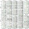 |
Fig. 1 On source CO spectra convolved to a ~20′′ beam. From left to right: 12CO 3–2, 10–9, 13CO 10–9, C18O 9–8, 5–4 and 10–9, respectively. Only the CO 3–2 lines are observed with the JCMT, the rest of the data are from Herschel-HIFI. The spectra are plotted by shifting the source velocity (Vlsr) to 0 km s-1 (actual source velocities are given in Table 4). The lines are shifted vertically. Intensity scale of some sources is multiplied by a constant value for easy viewing and marked if different from 1. The top half of the figure shows the Class 0 sources whereas the bottom part displays the Class I sources. The right-most column displays the C18O 5–4 and C18O 10–9 lines for the Class 0 sources only. The latter lines are very close to the H2O 312–303 line resulting in an intensity rise on the blue side of the spectrum in some sources. |
3. Results
3.1. CO line gallery
The 12CO, 13CO and C18O spectra from J = 2–1 up to J = 10–9 for each source are provided in Appendix C. This appendix contains figures of all the observed spectra and tables with the extracted information. Summary spectra are presented in Fig. 1 for the CO 3–2, 10–9, 13CO 10–9, C18O 5–4, 9–8, and 10–9 lines, respectively. Emission is detected in almost all transitions with our observing setup except some higher-J isotopolog lines discussed below. The high-J CO lines observed with Herschel are the first observations for these types of sources. Decomposition of line profiles is discussed in detail in San José-García et al. (2013) and is only briefly summarized below.
3.2. 12CO lines
12CO 10–9 emission is detected in all sources. Integrated and peak intensities are typically higher in the Class 0 sources compared with the Class I sources. Typical integrated intensities at the source positions range from 1 K km s-1 (in Oph IRS63) up to 82 K km s-1 (in Ser-SMM1), whereas peak intensities range from 0.6 K (in Oph IRS63) up to 9.3 K (in GSS30 IRS1). One striking result is that none of the 12CO 10–9 observations show self-absorption except for Ser-SMM1 and GSS30 IRS1, whereas all of the CO 3–2 observations have strong self-absorption, which suggests optically thick line centers6. The absorption components are located at the source velocities as indicated by the peak of the low-J C18O emission and are thus due to self-absorption from the outer envelope. Examining other available 12CO transitions (lower than J = 10–9) shows that the self-absorption diminishes with increasing J and disappears for all sources (again except Ser-SMM1 and GSS30 IRS1) at around J = 10–9 (see Figs. C.1–C.26).
Relative fractions of integrated intensities calculated for broad and narrow components in 12CO 10–9 lines.
For the 12CO lines, more than two thirds of the sample can readily be decomposed into two Gaussian components with line widths of ≤7.5 km s-1 (narrow) and 11–25 km s-1 (broad; see Fig. 2; San José-García et al. 2013, for details). The narrow component is due to the quiescent envelope whereas the broad component represents the swept-up outflow gas7. Figure 3 summarizes the relative fraction of each of the components in terms of integrated intensities (also tabulated in Table 2). For four sources in the sample, i.e., TMC1A, TMC1, Oph IRS63, and RNO91, the profiles could not be decomposed due to low S/N in their spectra. The fraction of emission contained in the narrow component ranges from close to 0% (IRAS 4A) to nearly 100% (L1527), with a median fraction of 42%. Particularly, for IRAS 4A, the narrow component is most likely hidden under the strong broad component, whereas for L1527, outflows are in the plane of the sky therefore the broad component is not evident. This decomposition demonstrates that the contributions from these two components are generally comparable so care must be taken in interpreting spectrally unresolved data from Herschel-SPIRE and PACS, and, to some extent, near-IR transitions of the same molecules.
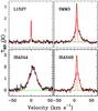 |
Fig. 2 Gaussian decomposition of the 12CO 10–9 profile toward four sources. The profile toward two sources, L1527 and IRAS 4A, can be decomposed into a single Gaussian, whereas SMM3, IRAS 4B and all the remaining sources in the sample require two components (decomposition shown with the dashed red fit). |
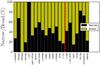 |
Fig. 3 Relative fraction of the integrated intensity of the narrow and broad components for each source. The 12CO 10–9 profile decomposition is given in San José-García et al. (2013). Yellow regions indicate the broad component fraction and black the narrow component fractions. The red dashed line divides the Class 0 (left) and Class I (right) sources. |
Figure 4 presents the averaged 12CO 3–2, 10–9, and H2O 110–101 lines for the Class 0 and Class I sources in order to obtain a generic spectral structure for one type of source. To compare with the H2O spectra, a similar averaging procedure was followed as in Kristensen et al. (2012), where ground state ortho-water composite spectra observed with Herschel-HIFI at 557 GHz were presented in a beam of 40″. In this comparison, the IRAS 15398 (Class 0), TMC1 and GSS30 IRS1 (Class I) spectra have been excluded from the averaging procedure. The CO 10–9 line of IRAS 15398 is taken at a position 15″ offset from the source position, the TMC1 spectrum was too noisy and the excitation of GSS30 IRS1 may not be representative of Class I sources (Kristensen et al. 2012). Therefore, 14 Class 0 and 9 Class I spectra are scaled to a common distance of 200 pc and averaged.
It is seen that the broad CO outflow component is much more prominent in the Class 0 than in the Class I sources (Fig. 4). For the Class 0 sources, the 10–9 line is broader than the 3–2 lines. However, neither is as broad as the line wings seen in H2O 557 GHz lines, for which the average H2O spectra are taken from Kristensen et al. (2012). The comparison between CO and H2O will be discussed further in Sect. 5.3.
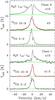 |
Fig. 4 Composite H2O 110–101, CO 10–9 and CO 3–2 spectra of Class 0 and Class I sources averaged in order to compare the line profiles of two types of sources. All spectra are rescaled to a common distance of 200 pc, shifted to the central 0 km s-1 velocity, rebinned to a 0.3 km s-1 velocity resolution. The CO spectra refer to a 20′′ beam, the H2O spectra to a 40′′ beam. The red spectra overlaid on top of the 12CO 10–9 are obtained by normalizing all the spectra to a common peak temperature first and then averaging them. |
For a few sources, high velocity molecular emission features associated with shock material moving at velocities up to hundred km s-1 have been observed (Bachiller et al. 1990; Tafalla et al. 2010). For species like SiO, their abundance is increased due to shock-induced chemistry (Bachiller & Perez Gutierrez 1997; Bourke et al. 1997). These Extremely High Velocity (EHV) components (or “bullet” emission) are also visible in the higher-J CO transitions, as well as in lower-J transitions, but the contrast in emission between bullet and broad outflow emission is greatly enhanced at higher frequencies. Bullets are visible specifically in CO 6–5 and 10–9 data toward L1448 mm and BHR71 at ~±60 km s-1 (see Fig. 5 for the bullets and Table 3 for the fit parameters). These bullets are also seen in H2O observations of the same sources, as well as other objects (Kristensen et al. 2011, 2012).
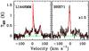 |
Fig. 5 12CO 10–9 spectra of L1448 mm and BHR71, where bullet structures are shown. The green lines indicates the baseline and the red lines represent the Gaussian fits of the line profiles. Fit parameters are given in Table 3. |
Fit parameters obtained from the bullet sources.
Source parameters.
3.3. 13CO lines
13CO emission is detected in all sources except for the 10–9 transition toward Oph IRS63, RNO91, TMC1A, and TMR1. The 10–9 integrated and peak intensities are higher in Class 0 sources compared with the Class I sources. Typical integrated intensities range from 0.1 K (L1527) up to 3.4 K km s-1 (Ser-SMM1). Peak intensities range from 0.1 K (L1448 MM, L1527) up to 0.4 K (Ser-SMM1). All 13CO 10–9 lines can be fitted by a single Gaussian (narrow component) except for Ser-SMM1 and IRAS 4A where two Gaussians (narrow and broader component) are needed.
Extracted rotational temperatures and column densities.
3.4. C18O lines
C18O emission is detected in all sources up to J = 5–4. The 9–8 line is seen in several sources, mostly Class 0 objects (BHR71, IRAS 2A, IRAS 4A, IRAS 4B, Ser-SMM1, L1551 IRS5). The C18O 10–9 line is detected after 5-hour integrations in IRAS 2A, IRAS 4A, IRAS 4B, Elias 29, GSS30 IRS1, and Ser-SMM1, with integrated intensities ranging from 0.05 (in IRAS 4A) up to 0.6 K km s-1 (Ser-SMM1). Peak intensities range from 0.02 K up to 0.07 K for the same sources. The rest of the high-J C18O lines do not show a detection but have stringent upper limits. The high S/N and high spectral resolution C18O 5–4 data reveal a weak, broad underlying component even in this minor isotopolog for several sources (see Fig. 1 in Yıldız et al. 2010).
The availability of transitions from 2–1 to 10–9 for many sources in optically thin C18O lines also gives an opportunity to revisit source velocities, Vlsr that were previously obtained from the literature. Table 4 presents the results with nine sources showing a change in Vlsr, compared with values listed in van Dishoeck et al. (2011) ranging from 0.2 km s-1 (IRAS 4A) up to 1.0 km s-1 (L1551-IRS5).
4. Rotational diagrams
To understand the origin of the CO emission, rotational diagrams provide a useful starting point to constrain the temperature of the gas. In our sample, we have CO and isotopolog emission lines of all sources from J = 2–1 up to 10–9 with upper level energies from Eup = 5 K to ~300 K. Rotational diagrams are constructed assuming that the lines can be characterized by a single excitation temperature Tex, also called rotational temperature Trot. Typically, the isotopolog 13CO and C18O lines are optically thin, as well as the 12CO line wings (see van Kempen et al. 2009b; Yıldız et al. 2012), so no curvature should be induced in their excitation diagrams due to optical depth effects. However, the low-J12CO line profiles have strong self-absorption and their cores are optically thick, leading to the column density of these levels being underestimated. The C18O 5–4 line has a beam size of 42″ and may thus contain unrelated cloud material, so its uncertainty is artificially enhanced from 10% to 20% in order to reduce its weight in the fit calculations.
Using the level energies, Einstein A coefficients and line frequencies from Table 1 and the cited databases, rotational diagrams are constructed where the column density for each level is plotted against its level energy (Goldsmith & Langer 1999). This temperature Trot is basically defined from the Boltzmann equation  (1)where Nu and Nl are the column densities in the upper and lower states, and gu and gl their statistical weights equal to 2Ju + 1 and 2Jl + 1, respectively. The CO column densities in individual levels are obtained from
 ![Mathematical equation: \begin{equation} \frac{N_{\rm u}}{g_{\rm u}} = \beta \frac{(\nu [\rm{GHz])^{2}}\, W [\mathrm{K\, km\, s^{-1}}]}{A_{\rm ul} [\rm s^{-1}]\, g_{\rm u}}, \end{equation}](/articles/aa/full_html/2013/08/aa20849-12/aa20849-12-eq106.png) (2)where β = 1937 cm-2 and
(2)where β = 1937 cm-2 and  is the integrated intensity of the emission line.
The slope of the linear fit to the observations, − (1/Trot), gives the rotational temperature, whereas the y-intercept gives the total column density ln (Ntotal/Q(Trot)) where Q(Trot) is the partition function referenced from CDMS for the temperature given by the fit.
The total integrated intensity W for each line is measured over the entire velocity range out to where line wings become equal to the 1σ noise. In L1448 mm and BHR71, the bullet emission is not included in the intensity calculation. In IRAS 2A, the emission in the 10–9 line is corrected for emission at one of the reference positions, which results in a higher Trot compared with Yıldız et al. (2012).
4.1. Rotational diagram results
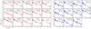 |
Fig. 6 Rotational diagrams for 12CO lines using the integrated intensities. All data are convolved to a 20″ beam and each plot shows the best single temperature fit to the observed transitions (see also Table 5). Left panel (red): Class 0 sources; right panel (blue): Class I sources. |
In Figs. 6–8, rotational diagrams are depicted for the 12CO, 13CO and C18O lines, respectively. Extracted excitation temperatures and column densities are presented in Table 5; 12CO column densities are not provided because they are affected by optical depth effects. In all sources the data can be fitted to a single temperature component from J = 2–1 up to 10–9 with a range of uncertainty from 12% to 21% except 13CO temperatures in Ced110-IRS4 and BHR71 where only two observations are present. Curvature is present for a number of sources which will be discussed in Sect. 4.3. The derived 12CO rotational temperatures range from ~50 K to ~100 K. The median temperatures for both Class 0 and Class I sources are similar, Trot = 71 K and 68 K, respectively.
For 13CO, the temperatures range from Trot ~35 K to ~60 K, with a median Trot = 46 K and 49 K for Class 0 and Class I sources, respectively. For C18O, the median temperature for Class 0 sources is Trot = 36 K. For Class I sources, either lack of observational data or non-detections make it harder to obtain an accurate temperature. Nevertheless, upper limits are still given. The median Trot for the sources with ≥3 data points is 37 K. A summary of the median rotational temperatures is given in Table 6. Figure 9 presents the 12CO and 13CO temperatures in histogram mode for the Class 0 and Class I sources, with no statistically significant differences between them. Note that this analysis assumes that all lines have a similar filling factor in the ~20′′ beam; if the higher-J lines would have a smaller filling factor than the lower-J lines the inferred rotational temperatures would be lower limits.
Median rotational temperatures and colum densities of Class 0 and Class I sources calculated from 12CO, 13CO and C18O.
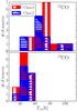 |
Fig. 9 Distribution of rotation temperatures (Trot) calculated from 12CO and 13CO line observations. The median temperatures are listed in Table 6. |
For the case of Serpens-SMM1, our inferred rotational temperatures of 97 ± 12 and 60 ± 8 K compare well with those of 103 ± 15 and 76 ± 6 K found by Goicoechea et al. (2012) from Herschel-SPIRE data for 12CO and 13CO, respectively. The SPIRE values were obtained from a fit to the Ju = 4−14 levels, with the beam changing by a factor of ~3 from ~47″ to ~13″ across the ladder.
The 12CO and 13CO 2–1 lines included in Figs. 6 and 7 are observed in a similar ~20″ beam as the higher transitions, but they most likely include cold cloud emission as well. Removing those lines from the rotational diagrams increases the temperatures around 10–15 %. Similarly, the C18O 5–4 line is observed in a 42″ beam and removing this line from the fit increases the temperatures around 5–10%, which is still within the error bars. In practice, we did not discard the C18O 5–4 observations but increased their uncertainty to give them less weight in the calculations. The effect of multiple velocity components in discussed in Sect. 4.4.
The 13CO and C18O column densities are converted to 12CO column densities by using 12C/13C = 65 (based on Langer & Penzias 1990; Vladilo et al. 1993) and 16O/18O = 550 (Wilson & Rood 1994) and then using CO/H2 = 10-4 to obtain the H2 column density (tabulated in Table 5). The median H2 column densities for Class 0 sources are 4.6 × 1021 cm-2 and 5.2 × 1021 cm-2 for 13CO and C18O data, respectively. For Class I sources the value is 4.6 × 1021 cm-2 for 13CO, with the caveat that only few Class I sources have been measured in C18O. The agreement between the two isotopologs indicates that the lines are not strongly affected by optical depths. Since this conversion uses a CO/H2 abundance ratio close to the maximum, the inferred H2 column densities should be regarded as minimum values. In particular, for Class 0 sources freeze-out and other chemical processes will lower the CO/H2 abundance (see Sect. 6) (Jørgensen et al. 2002). Thus, the actual difference in column densities between the Class 0 and Class I stages is larger than is shown in Table 5.
4.2. CO ladders
Spectral Line Energy Distribution (SLED) plots are another way of representing the CO ladder where the integrated flux is plotted against upper level rotational quantum number, Jup. In Fig. 10, 12CO line fluxes for the observed transitions are plotted. Since the CO 3–2 lines are available for all sources, the fluxes are all normalized to their own CO 3–2 flux. The thick blue and red lines are the median values of all sources for each transition for each class. It is readily seen that the Class 0 and Class I sources in our sample have similar excitation conditions, but that the Class I sources show a wider spread at high-J and have higher error bars due to the weaker absolute intensities. Similarly, as can be inferred from Fig. 9, the 13CO SLEDs do not show any significant difference between the two classes. Thus, although the continuum SEDs show a significant evolution from Class 0 to Class I with Tbol increasing from <30 K to more than 500 K, this change is not reflected in the line SLEDs of the 12CO or the optically thinner 13CO excitation. This limits the usage of CO SLEDs as an evolutionary probe. One of the explanations for this lack of evolution is that Tbol depends on thermal emission from both the dust in the envelope and the extincted stellar flux, whereas the SLED only traces the temperature of the gas in the envelope and/or outflow, but has no stellar component. Moreover, the infrared dust emission comes from warm (few hundred K) optically thick dust very close to the protostar, whereas, the CO originates further out the envelope.
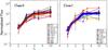 |
Fig. 10 12CO spectral line energy distribution (SLED) for the observed transitions. All of the fluxes are normalized to their own CO 3–2 flux for Class 0 (left) and Class I (right) sources separately. The beams are ~20′′ beam. The thick lines are the median values of each transitions. |
4.3. Two temperature components?
Unresolved line observations of higher-J CO transitions (J = 13 up to 50) by Herschel-PACS (Herczeg et al. 2012; Karska et al. 2013; Manoj et al. 2013) typically show two temperature components with ~300 K and ~900 K. Goicoechea et al. (2012) found three temperature components from combined SPIRE and PACS data, with the lower temperature of ~100 K fitting lines up to Ju = 14, similar to that found in our data. The question addressed here is if the higher 300 K component only appears for lines with Ju > 10 or whether it becomes visible in our data. One third of our sample shows a positive curvature in the 12CO rotation diagrams (Fig. 6), specifically IRAS 4A, IRAS 4B, BHR71, IRAS 15398, L483mm, Ser-SMM1, L723mm, B335, and L1489 (see Fig. 11).
The curvature in 12CO rotation diagrams is treated by dividing the ladder into two components, where the first fit is from 2–1 to 7–6 for the colder component and the second fit from 7–6 to 10–9 for the warmer component. The fit from 2–1 to 10–9 is named as global. The median Trot is 43 K for the colder component and 138 K for the warmer component for these nine sources.
Close inspection of the SPIRE data by Goicoechea et al. (2012) shows a slight curvature for low-J in their cold component as well. The “two-component” decomposition is perhaps a generic feature for Class 0 low-mass protostars, which implies that the CO 10–9 transition is at the border of the transitions for the cold (Trot < 100 K) and warm (Trot ~ 300 K) component associated with the currently shocked gas (Karska et al. 2013). Trot clearly increases when higher rotational levels are added (Fig. 11), and for the brightest sources in NGC 1333 and Serpens, Trot > 150 K. See Sect. 4.4 for further discussion.
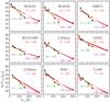 |
Fig. 11 Two temperature components fitted for selected sources to the 12CO lines, from 2–1 to 7–6 (cold), from 7–6 to 10–9 (warm), and 2–1 to 10–9 (global). |
4.4. Velocity resolved diagrams
To investigate whether the 12CO narrow and broad components have different temperatures, Fig. 12 presents excitation temperatures calculated channel by channel for a few sources with high S/N. Each spectrum is shifted to Vlsr = 0 km s-1 and rebinned to 3 km s-1 velocity resolution. It is obvious from Fig. 1 that the line wings are more prominent in the CO 10–9 transitions, specifically for Class 0 sources, as is reflected also in the increasing line widths with the increasing rotation level (see Figs. C.1–C.26; San José-García et al. 2013). Figure 12 shows that in the optically thin line wings, the excitation temperatures are a factor of 2 higher than in the line centers implying that the wings of the higher-J CO lines are associated with the warmer material described in Sect. 4.3. Since the presence of self-absorption at line centers of the lower-J lines reduces their emission, the excitation temperatures at low velocities are further decreased if this absorption is properly corrected for.
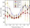 |
Fig. 12 Rotational temperatures calculated channel by channel for 12CO. Each spectrum is shifted to Vlsr = 0 km s-1 and rebinned to 3 km s-1 velocity resolution. |
Another way to illustrate the change with velocity is to look at the CO 10–9 and CO 3–2 spectra for each source as shown in Fig. A.1. Figure 13 shows the blue and red line-wing ratios for the 14 sources with the highest S/N. For all sources, the line ratios increase with increasing velocity, consistent with Fig. 12.
In summary, while a single rotational temperature provides a decent fit to the bulk of the CO and isotopolog data, both the 12CO integrated intensity rotational diagrams and the velocity resolved diagrams indicate the presence of a second, highly excited component for Class 0 sources. This warmer and/or denser component is most likely associated with the broad line wings, as illustrated by the 10–9/3–2 line ratios, whereas the colder component traces the narrow quiescent envelope gas. On average, the integrated intensities have roughly equal contributions from the narrow and broad components (Fig. 3) so the single rotational temperatures are a weighted mean of the cold and warmer values.
4.5. Kinetic temperature
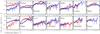 |
Fig. 13 Ratios of the CO 10–9/3–2 line wings for 14 protostars as function of velocity offset from the central emission. Spectra are shifted to Vlsr = 0 km s-1. The wings start at ±2.5 km s-1 from Vlsr in order to prevent adding the central self-absorption feature in the CO 3–2 lines. |
Having lines from low-to-high-J CO provides information about the physical conditions in the different parts of the envelope. The critical densities for the different transitions are ncr = 4.2 × 105 cm-3, 1.2 × 105 cm-3, and 2 × 104 cm-3 for CO 10–9, 6–5 and 3–2 transitions at ~50–100 K, using the CO collisional rate coefficients by Yang et al. (2010). For densities higher than ncr, the emission is thermalized and therefore a clean temperature diagnostic, however, for lower densities the precise value of the density plays a role in the analysis. In the high density case (n > ncr), the kinetic temperature is equal to the rotation temperature. By using two different 12CO lines, kinetic temperatures can be calculated if the density is known independently using the RADEX non-LTE excitation and radiative transfer program (van der Tak et al. 2007). The analysis below for CO 10–9/3–2 assumes that the emission originates from the same gas.
The resulting model line ratios are presented in Fig. 14 for a grid of temperatures and densities. Densities for each source are calculated from the envelope parameters determined by modeling of the submillimeter continuum emission and spectral energy distribution (Kristensen et al. 2012). A spherically symmetric envelope model with a power-law density structure is assumed (Jørgensen et al. 2002). The 20″ diameter beam covers a range of radii from ~1250 AU (e.g., Ced110IRS4, Oph sources) up to 4500 AU (HH46) and the densities range from 5.8 × 104 cm-3 (Elias 29) up to 2.3 × 106 cm-3 (Ser-SMM4). The densities for all sources at the 10″ radius are given at the last column in Table 4. Note that these are lower limits since the densities increase inward of 10′′. The envelope densities are used here as a proxy for the densities at the outflow walls where the entrainment occurs.
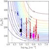 |
Fig. 14 Model CO 10–9/3–2 line intensity ratios as function of temperature and density, obtained for a CO column density of 1016 cm-2 with line-widths of 10 km s-1, representative of the observed CO intensity and line width. Note that the bars are the ranges of lower and upper limits as seen from the observations in Fig. 13. Red markers are for Class 0 and blue markers are for Class I sources. Blue wing ratios are indicated with triangles and red wing ratios have square symbols. Thick magenta and black lines indicate the ratios from the composite spectra for Class 0 and Class I sources, respectively. Vertical dashed lines indicate the limits for ncr for CO 3–2 (brown) and CO 10–9 (green). In the relevant density range, higher ratios are indicative of higher kinetic temperatures. |
The majority of the Class 0 sources have densities that are similar or higher than the critical densities of the high-J CO lines, with the possible exceptions of Ced110-IRS4, L483 mm, L723 mm, and L1157. However, in Class I sources, the majority of the densities are lower than the critical densities with the exception of L1551 IRS5. The inferred kinetic temperatures from the CO 10–9/3–2 blue and red line-wings, which generally increase with velocity, are presented in Table 5 and range mostly from 70 K to 250 K. The ratios for individual sources are included in Fig. 14 at the 10′′ radius density of the sources.
The thick magenta and black bars indicate the average values for the composite Class 0 and Class I sources (Sect. 5.3). For average densities at a 10″ radius of ~106 cm-3 and ~105 cm-3 for Class 0 and Class I sources, respectively, the CO 10–9/CO 3–2 line ratios would imply kinetic temperatures of around 80–130 K for Class 0 and 140–180 K for Class I sources (Fig. 14), assuming the two lines probe the same physical component. If part of the CO 10–9 emission comes from a different physical component, these values should be regarded as upper limits.
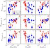 |
Fig. 15 From top to bottom, 12CO 10–9, 13CO 10–9, and C18O 3–2 integrated intensity W normalized at 200 pc are plotted against various physical properties: envelope mass at 10 K radius, Menv; bolometric temperature, Tbol; and bolometric luminosity, Lbol. Green lines are the best fit to the data points and r values in each of the plots are Pearson correlation coefficient. |
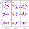 |
Fig. 16 Calculated rotational temperatures, Trot, plotted Menv, Tbol, and Lbol, for 12CO (top), 13CO (middle), C18O lines (bottom). The median excitation temperatures of ~70 K, 48 K and 37 K for 12CO, 13CO and C18O, respectively, are indicated with the green dashed lines. Typical error bar for each of the Trot values is shown in the upper left plot, represented in black circle data point. In the C18O plots, blue arrows indicate the upper limits for a number of sources. These figures are compared with disk evolution models of Harsono et al. (2013, magenta solid lines), which represents all three models discussed in the text. Magenta arrows also show the direction of time. The figures show that the excitation temperature does not change with the increasing luminosity, envelope mass or density, confirming that Class 0 and I sources have similar excitation conditions. |
5. Correlations with physical properties
5.1. Integrated intensities
Figure 15 shows the integrated intensities W of the CO 10−9 lines plotted against Lbol, Menv, and Tbol. The intensities are scaled to a common distance of 200 pc. The bolometric luminosity, Lbol and bolometric temperature Tbol of the sources have been measured using data from infrared to millimeter wavelengths including new Herschel far-infrared fluxes, and are presented in Kristensen et al. (2012). These are commonly used evolutionary tracers in order to distinguish young stellar objects. The envelope mass, Menv is calculated from the DUSTY modeling by Kristensen et al. (2012).
In Fig. 15, the green lines are the best power-law fits to the entire data set. Clearly, the CO 10–9 lines are stronger for the Class 0 sources which have higher Menv and Lbol and lower Tbol, for all isotopologs. The same correlation is seen for other (lower-J) CO and isotopolog lines, such as CO 2–1, 3–2, 4–3, 6–5 and 7–6; examples for 13CO 10–9 and C18O 3–2 are included in Fig. 15. The Pearson correlation coefficients for 12CO 10–9 are r = 0.39 (1.87σ), 0.81 (4.05σ), and − 0.36 (− 1.68σ) for Lbol, Menv, and Tbol, respectively. The coefficients, r, for Menv in 13CO 10–9 and C18O 3–2 are 0.90 (4.49σ) and 0.59 (2.97σ). Those correlations indicate that there is a strong correlation between the intensities and envelope mass, Menv, consistent with the lines becoming weaker as the envelope is dissipated. Together with the high-J CO lines, the C18O low-J lines are also good evolutionary tracers in terms of Menv and Tbol. Adding intermediate and high-mass WISH sources to extend the correlation to higher values of Lbol and Menv shows that these sources follow the same trend with similar slopes with a strong correlation (San José-García et al. 2013). The scatter in the correlation partly reflects the fact that the CO abundance is not constant throughout the envelope and changes with evolutionary stage (see Sect. 6).
5.2. Excitation temperature and comparison with evolutionary models
Figure 16 presents the derived rotational temperatures for 12CO, 13CO and C18O versus Menv, Tbol, and Lbol. In contrast with the integrated intensities, no systematic trend is seen for any parameter. As noted in Sect. 4.2, this lack of change in excitation temperature with evolution is in stark contrast with the evolution of the continuum SED as reflected in the range of Tbol.
To investigate whether the lack of evolution in excitation temperature is consistent with our understanding of models of embedded protostars, a series of collapsing envelope and disk formation models with time has been developed by Harsono et al. (2013), based on the formulation of Visser et al. (2009) and Visser & Dullemond (2010). Three different initial conditions are studied. The total mass of the envelope is taken as 1 M⊙ initially in all cases, but different assumptions about the sound speed cS and initial core angular momentum Ω result in different density structures as a function of time. The three models have Ω = 10-14, 10-14, 10-13 s-1 and cS = 0.26, 0.19, 0.26 km s-1, respectively, covering the range of parameters expected for low-mass YSOs. The luminosity of the source changes with time from <1 to ~5–10 L⊙. The dust temperature is computed at each time step using a full 2D radiative transfer model and the gas temperature is taken equal to the dust temperature.
Given the model physical structures, the CO excitation is then computed as a function of time (evolution) through full 2D non-LTE excitation plus radiative transfer calculations. The line fluxes are computed for i = 45° inclination but do not depend strongly on the value of i. The resulting line intensities are convolved to a 20′′ beam and CO rotational temperatures are computed using the 2–1 up to 10–9 lines. Details are provided in Harsono et al. (2013). The resulting model excitation temperatures are plotted against model Lbol, Tbol, and Menv values as a function of time, with envelope mass decreasing with time. Note that because these models were run for a single Menv = 1 M⊙, they do not cover the full range of observed Menv.
The first conclusion from this comparison is that the model rotational temperatures hardly show any evolution with time consistent with the observations, in spite of the envelope mass changing by two orders of magnitude. Although the density decreases to values below the critical densities, the temperature increases throughout the envelope so the rotational temperatures stay constant.
The second conclusion is that the model rotational temperatures are generally below the observed temperatures, especially for 12CO (~55 K) and 13CO (~36 K). For 12CO this could be due to the fact that outflow emission is not included in the models, which accounts typically for more than half of the line intensity and has a higher rotational temperature (see Sect. 4.4). Indeed, the rotational temperature of the narrow component is around 60–70 K, closer to the model values. For 13CO, the model Trot values could be lower than the observed values because UV photon heating contributes along the outflow walls (see Visser et al. 2012; Yıldız et al. 2012, for quantitative discussion), although this effect may be small within ~1000 AU radius of the source position itself (Yıldız et al. 2012). The model C18O rotational temperatures are close to the observed values (typically 28–35 K), illustrating that the envelope models are an accurate representation of the observations.
5.3. High-J CO vs. water
Do the average spectra of the Class 0 and Class I sources show any evolution and how does this compare with water? In Fig. 4, stacked and averaged 12CO 3–2, 10–9, and H2O 110–101 spectra for the Class 0 and I sources have been presented. Consistent with the discussion in Sect. 3.2 and San José-García et al. (2013), Class 0 sources have broader line widths than Class I sources, showing the importance of protostellar outflows in Class 0 sources. In general, Class I sources show weaker overall emission except for the bright sources GSS30 IRS1 and Elias 29, consistent with the trend in Fig. 15. Figure 17 shows the H2O 110–101/CO 10–9, H2O 110–101/CO 3–2, and CO 10–9/CO 3–2 line ratios of the averaged spectra. The CO 10–9/CO 3–2 line wings show increasing ratios from ~0.2 to ~1.0–3.0 for the averaged Class 0 spectrum, but this trend is weaker for the Class I sources which have a near constant ratio of 0.3. The implied kinetic temperature has been discussed in Sect. 4.5.
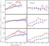 |
Fig. 17 Blue and red line wing ratios of CO 10–9/3–2 (top panel), H2O 110–101/CO 10–9 (middle panel), and H2O 110–101/CO 3–2 (bottom panel) for the composite Class 0 and Class I source spectra. The H2O/CO 10–9 and H2O/CO 3–2 ratios are a factor of two lower than shown in Fig. 4 due to the beam size difference of 20″ (CO 10–9 lines) to 40″ (H2O 110–101 lines). |
Franklin et al. (2008) examined the H2O abundance as a function of velocity by using CO 1–0 as a reference frame. Here it is investigated how H2O/CO line ratios change with increasing J by using CO 3–2 and 10–9 as reference frames (Fig. 17). In this figure, the CO 3–2 line has been convolved to a 40″ beam using the JCMT data (also done by Kristensen et al. 2012). For the 10–9 line, no map is available so the emission is taken to scale linearly with the beam size, as appropriate for outflow line wings assuming a 1D structure (Tafalla et al. 2010). Thus, the 10–9 intensities are a factor of two lower than those shown in, for example, Fig. 4 where data in a 20″ beam were used. The line wing ratios are computed up to the velocity where the CO emission reaches down to ~2σ noise limit, even though the H2O line wings extend further.
Consistent with Kristensen et al. (2012), an increasing trend of H2O/CO 3–2 line ratios with velocity is found for both Class 0 and Class I sources. However, the H2O/CO 10–9 ratios show little variation with velocity for Class 0 sources, and the ratio is constant within the error bars. For the Class I sources an increasing trend in H2O/CO 10–9 line ratios is still seen.
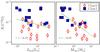 |
Fig. 18 Constant abundance profiles are fitted to the lower-J C18O 3–2 are shown as function of Lbol and Menv. Green lines are the best fit to the data points and r values in each of the plots are Pearson correlation coefficient. |
Because of the similarity of the CO 10–9 line wings with those of water, it is likely that they are tracing the same warm gas. This is in contrast with the 3–2 line, which probes the colder entrained gas. The conclusion that H2O and high-J CO emission go together (but not low-J CO) is consistent with recent analyses (Santangelo et al. 2012; Vasta et al. 2012; Tafalla et al. 2013) of WISH data at outflow positions offset from the source. The CO 10–9 line seems to be the lowest J transition whose line wings probe the warm shocked gas rather than the colder entrained outflow gas (see also Sect. 4.3); HIFI observations of higher-J lines up to J = 16–15 should show an even closer correspondence between H2O and CO (Kristensen et al., in prep.). That paper will also present H2O/CO abundance ratios since deriving those from the data requires further modeling because the H2O lines are subthermally excited and optically thick.
6. CO abundance and warm inner envelope
6.1. CO abundance profiles
The wealth of high quality C18O lines probing a wide range of temperatures allows the CO abundance structure throughout the quiescent envelope to be constrained. The procedure has been described in detail in Yıldız et al. (2010, 2012). Using the density and temperature structure of each envelope as derived by Kristensen et al. (2012, their Table C.1; see Sect. 4.5, the CO abundance profile can be inferred by comparison with the C18O data. The Ratran (Hogerheijde & van der Tak 2000) radiative-transfer modeling code is used to compute line intensities for a given trial abundance structure.
Six sources with clear detections of C18O 9–8 and 10–9 have been modeled. The outer radius of the models is important for the lower-J lines and for Class 0 sources. It is taken to be the radius where either the density n drops to ~1.0 × 104 cm-3, or the temperature drops below 8–10 K, whichever is reached first. In some Class 0 sources (e.g., IRAS 4A, IRAS 4B), however, the density is still high even at temperatures of ~8 K; here the temperature was taken to be constant at 8 K and the density was allowed to drop until ~104 cm-3. The turbulent velocity (Doppler-b parameter) is set to 0.8 km s-1, which is representative of the observed C18O line widths for most sources (Jørgensen et al. 2002) except for Elias 29 where 1.5 km s-1 is adopted. The model emission is convolved with the beam in which the line has been observed.
Summary of C18O abundance profiles.
First, constant abundance profiles are fitted to the lower-J C18O 3–2, together with the 2–1 transitions, if available and they are tabulated in Table 5. In Fig. 18, these abundances are plotted as function of bolometric luminosities and envelope masses. Consistent with Jørgensen et al. (2002), Class 0 sources with higher envelope mass have lower average abundances in their envelopes than Class I sources, by more than an order of magnitude. This result is firm for lower-J transitions; however, in order to fit higher-J lines simultaneously, it is necessary to introduce a more complex “drop” abundance profile with a freeze-out zone (Jørgensen et al. 2004). The inner radius is determined by where the dust temperature falls below the CO evaporation temperature of 25 K. The outer radius is determined by where the density becomes too low for freeze-out to occur within the lifetime of the core.
Following Yıldız et al. (2010, 2012) for the NGC 1333 IRAS 2A, IRAS 4A and IRAS 4B protostars, such a drop-abundance profile provides a better fit to the C18O data than a constant or “anti-jump” abundance. In these profiles, Xin is defined as the abundance of the inner envelope down to the evaporation temperature of CO, Tev. The outer abundance X0 is set to 5 × 10⁻⁷ below at a certain desorption density, nde, corresponding to the maximum expected CO abundance of 2.7 × 10⁻⁴. The drop abundance zone is defined as the freeze-out region in the envelope between the limit of Tev and nde (see Fig. B.1 in Yıldız et al. 2010.) Best fit abundances for different sources are summarized in Table 7. As in our previous work and in Fuente et al. (2012) and Alonso-Albi et al. (2010), the CO abundance in the inner envelope is below the canonical value of 2.7 × 10⁻⁴ (Lacy et al. 1994) by a factor of a few for the Class 0 sources, probably due to processing of CO to other species on the grains during the cold phase.
Only two of the Class I sources (GSS30 IRS1 and Elias 29) have been observed in deep integrations of C18O 10–9 and therefore they are the only Class I sources modeled in detail. These sources are located in the Ophiuchus molecular cloud, where two low-density foreground sheets contribute to the lowest J 1–0 and 2–1 lines (e.g., Loren 1989; van Kempen et al. 2009d). To take this into account, a single slab foreground cloud is added in front of the protostars with 15 K temperature, 1.5 × 104 cm-3 H2 density, and 1016 cm-2 CO column density. Best-fit models for the C18O 3–2, 5–4, 9–8and 10–9 lines toward GSS30 IRS1 and Elias 29 can then be well fit with a constant CO abundance close to the canonical value and require at most only a small freeze-out zone (for the case of GSS30 IRS1). Jørgensen et al. (2005b) argue that the size of the freeze-out zone evolves during protostellar evolution, i.e., for Class 0 sources the drop-zone should be much larger than for Class I sources. This is indeed consistent with the results found here. Interestingly, however, the constant or inner abundances Xin are high, consistent with the maximum CO gas phase abundance. If these Class I sources went through a previous Class 0 phase with a more massive and colder envelope, apparently less CO ice has been converted to other species during this phase than found for the NGC 1333 sources. One possible explanation is that the dust in this part of Ophiuchus is on average warmer due to the UV radiation from the nearby massive stars. Higher dust temperatures decrease the efficiency of CO hydrogenation because the hydrogen atom has only a short residence time on the grain (Fuchs et al. 2009). Alternatively, the low CO abundance component may have been incorporated to the disk and/or dispersed. Finally, there may be a PDR contribution to the observed intensities (Liseau et al. 2012; Bjerkeli et al. 2012).
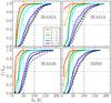 |
Fig. 19 Cumulative intensity I/Itot for various C18O lines as function of envelope radius (as indicated by the temperature To) with the dust opacity included (solid curves), and dust opacity off (dashed curves). The dash-dotted lines indicates the fractions of 50 and 80%, respectively. |
6.2. Warm inner envelope
The higher-J C18O transitions such as 9–8 and 10–9 (Eu up to ~300 K) in principle trace directly the warmer gas in the inner envelope. Can we now use these data to put limits on the amount of warm >100 K gas, which could then be used as a reference for determining abundances of complex molecules?
In principle, one could argue that simply summing the observed column density of molecules in each level should provide the total warm column density, as done by Plume et al. (2012) for the case of Orion and in Table 5 based on the rotational diagrams. However, in the low-mass sources considered here freeze-out also plays a role and CO can be converted to other species on the grains. Thus, to convert to N(H2) in the warm gas, one needs to use the values of Xin that have been derived in Table 7. However, these values are derived in the context of a physical model of the source, so in principle one simply recovers the input model.
Besides the complication of the changing CO abundance with radius, there are two other effects that make a direct observational determination of the warm H2 column densities far from simple. The first issue is the fact that not all emission in the 9–8 or 10–9 lines arises from gas at >100 K even though Eu = 237–290 K. Figure 19 shows the cumulative C18O line intensities (solid curves) as functions of radius (or, equivalently, temperature) for four source models. Itot are the intensities measured from the best-fit abundance models as tabulated in Table 7. Thus, the curves represent the fraction of line intensities which have their origins in gas at temperatures below T0 for the different transitions. As expected, about 90–95% of the C18O emission in the lower-J transitions up to Ju ≤ 3 comes from gas at <40 K. However, even for the 9–8 transition, 30–50% comes from gas at less than 50 K whereas only ~10–20% originates at temperatures above 100 K. For the 10–9 transition, ~20–40% of the emission comes from >100 K. Thus, these are additional correction factors that would have to be applied to obtain the columns of gas >100 K.
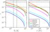 |
Fig. 20 Dust optical depth at 1 THz as function of envelope radius and temperature. Horizontal dashed lines indicate the τ = 1 and τ = 0.1 values whereas vertical dash-dotted lines are radii, where the temperatures are between 40 K and 60 K. |
A second potential issue is that the dust continuum at 1 THz may become optically thick so that warm C18O emission cannot escape. Figure 20 shows the dust opacity as function of radius throughout the envelope, obtained by multiplying the column densities with the κdust(1 THz) (Ossenkopf & Henning 1994, their Table 1, Col. 5) and integrating from the outer edge to each radius to find the optical depth (τ). It is seen that the dust is optically thin (τ < 1 at 1 THz) throughout the envelopes of our sources except for IRAS 4A, where it reaches unity in the innermost part of the envelope. To what extent is the fraction of high-J emission coming from >100 K affected by the dust? In Fig. 19 (dashed curves), the dust emission has been turned off in the Ratran models. For the lower-J, lower-frequency transitions, almost no difference is found; however, for the higher-J transitions the cumulative intensities are somewhat higher (up to a factor of 2) when no dust is present.
In summary, there are various arguments why warm H2 column densities cannot be inferred directly from the high-J C18O data. Moreover, all of these arguments use a simple spherically symmetric physical model of the source to quantify the effects. It is known that such models fail on the smaller scales (less than a few hundred AU) due to the presence of a (pseudo)disk and outflow cavities (e.g., Jørgensen et al. 2005a). Spatially resolved data are needed to pin down the structure of the inner envelopes and properly interpret the origin of the high-J C18O emission.
7. Conclusions
We have presented the first large-scale survey of spectrally resolved low- to high-J CO and isotopolog lines (2 ≤ Jup ≤ 10) in 26 low-mass young stellar objects by using data from Herschel-HIFI, APEX, and JCMT telescopes. Velocity resolved data are the key to obtaining the complete picture of the protostellar envelope and the interaction of the protostar with the environment and follow the evolution from the Class 0 to Class I phase.
-
The 12CO line profiles can be decomposed into narrow and broadcomponents, with the relative fractions varying from zero tonearly 100%, with a median of 42% of the J =10–9 emission in the narrow component. Theaverage Class 0 rofile shows abroader, more prominent wing than the averageClass I profile.
-
The 10–9 together with 3–2 intensities correlate strongly with total luminosity Menv and are inversely proportional with bolometric temperature Tbol, illustrating the dissipation of the envelope with evolution.
-
Rotation diagrams are constructed for each source in order to derive rotational temperatures and column densities. Median temperatures of Trot are 70 K, 48 K, and 37 K, for the 12CO, 13CO and C18O transitions, respectively, for integrated intensities over the entire line ptofiles. The excitation temperatures and SLEDs are very similar for Class 0 and Class I sources in all three isotopologs and do not show any trend with Menv, Lbol or Tbol, in contrast with the continuum SEDs.
-
The 12CO 10–9/CO 3–2 intensity ratio as well as the overall rotational temperature generally increase with velocity. The central narrow component due to the quiescent envelope has a lower temperature than the broad outflow component.
-
Models of the CO emission from collapsing envelopes reproduce the lack of evolution found in the observed excitation temperatures. They agree quantitatively for C18O but underproduce the 12CO and 13CO excitation temperatures, pointing to the combined effects of outflows and photon-heating in boosting these temperatures.
-
Comparison of the 12CO profiles with those of H2O shows that the H2O 110–101/CO 10–9 intensity ratio is nearly constant with velocity for Class 0 sources, contrary to the case for low-J CO lines. Combined with other findings, this suggests that the CO 10–9 line has contributions from the warmer (~300 K) shocked gas seen in PACS data containing also water, rather than the colder (~100 K) entrained outflow gas traced by low-J CO lines.
-
The C18O line intensities give average CO abundances that increase by more than an order of magnitude with decreasing envelope mass from the Class 0 to the Class I phase, consistent with earlier findings. Modeling of the full set of higher-J C18O lines within a given physical model shows further evidence for a freeze-out zone (“drop” abundance profile) in the envelopes of Class 0 sources with an inner CO abundance that is a factor of a few lower than the canonical CO abundance probably due to processing of CO on grains into other molecules. For two Class I sources in Ophiuchus, no freeze-out zone is needed and the data are consistent with a constant high abundance value at a level that is close to the maximum gas-phase CO abundance. The lack of processing for these sources may de due to the higher dust temperatures in Ophiuchus, evolutionary effects, or a PDR contribution.
-
The warm (>100 K) H2 column densities cannot be derived directly from C18O 9–8 or 10–9 lines because of contributions to the emission from colder gas in the envelope, dust extinction at high frequency, and more generally a lack of knowledge of the source structure on a few hundred AU scales.
Overall, our data show that the evolution from the Class 0 to the Class I phase is traced in the decrease of the line intensities reflecting envelope dissipation, a less prominent broad wing indicating a decrease in the outflow power, and an increase in the average CO abundance, reflecting a smaller freeze-out zone. The CO excitation temperature from Ju = 2 to 10 shows little evolution between these two classes, however.
The next step in the study of CO in low mass protostars is clearly to obtain higher spectral and spatial resolution data with instruments like ALMA that recover the full range of spatial scales from <100 AU to >1000 AU in both low- and high-J CO and isotopolog lines.
Online material
Appendix C: CO spectra of sample
Appendix C.1: L1448MM
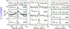 |
Fig. C.1 Observed 12CO, 13CO, and C18O transitions for L1448MM. |
Observed line intensities for L1448MM in all observed transitions.
Appendix C.2: IRAS2A
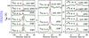 |
Fig. C.2 Observed 12CO, 13CO, and C18O transitions for IRAS 2A. |
Observed line intensities for IRAS 2A in all observed transitions.
Appendix C.3: IRAS4A
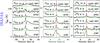 |
Fig. C.3 Observed 12CO, 13CO, and C18O transitions for IRAS 4A. |
Observed line intensities for IRAS4A in all observed transitions.
Appendix C.4: IRAS4B
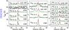 |
Fig. C.4 Observed 12CO, 13CO, and C18O transitions for IRAS 4B. |
Observed line intensities for IRAS4B in all observed transitions.
Appendix C.5: L1527
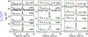 |
Fig. C.5 Observed 12CO, 13CO, and C18O transitions for L1527. |
Observed line intensities for L1527 in all observed transitions.
Appendix C.6: Ced110IRS4
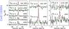 |
Fig. C.6 Observed 12CO, 13CO, and C18O transitions for Ced110-IRS4. |
Observed line intensities for Ced110-IRS4 in all observed transitions.
Appendix C.7: BHR71
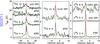 |
Fig. C.7 Observed 12CO, 13CO, and C18O transitions for BHR71. |
Observed line intensities for BHR71 in all observed transitions.
Appendix C.8: IRAS153981
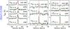 |
Fig. C.8 Observed 12CO, 13CO, and C18O transitions for IRAS15398. |
Observed line intensities for IRAS15398 in all observed transitions.
Appendix C.9: L483 mm
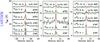 |
Fig. C.9 Observed 12CO, 13CO, and C18O transitions for L483 mm. |
Observed line intensities for L483 mm in all observed transitions.
Appendix C.10: SMM1
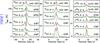 |
Fig. C.10 Observed 12CO, 13CO, and C18O transitions for SerSMM1. |
Observed line intensities for SerSMM1 in all observed transitions.
Appendix C.11: SMM4
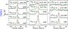 |
Fig. C.11 Observed 12CO, 13CO, and C18O transitions for SerSMM4. |
Observed line intensities for SerSMM4 in all observed transitions.
Appendix C.12: SMM3
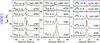 |
Fig. C.12 Observed 12CO, 13CO, and C18O transitions for SerSMM3. |
Observed line intensities for SerSMM3 in all observed transitions.
Appendix C.13: L723 mm
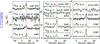 |
Fig. C.13 Observed 12CO, 13CO, and C18O transitions for L723 mm. |
Observed line intensities for L723 mm in all observed transitions.
Appendix C.14: B335
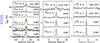 |
Fig. C.14 Observed 12CO, 13CO, and C18O transitions for B335. |
Observed line intensities for B335 in all observed transitions.
Appendix C.15: L1157
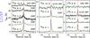 |
Fig. C.15 Observed 12CO, 13CO, and C18O transitions for L1157. |
Observed line intensities for L1157 in all observed transitions.
Appendix C.16: L1489
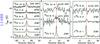 |
Fig. C.16 Observed 12CO, 13CO, and C18O transitions for L1489. |
Observed line intensities for L1489 in all observed transitions.
Appendix C.17: L1551IRS5
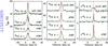 |
Fig. C.17 Observed 12CO, 13CO, and C18O transitions for L1551IRS5. |
Observed line intensities for L1551IRS5 in all observed transitions.
Appendix C.18: TMR1
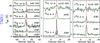 |
Fig. C.18 Observed 12CO, 13CO, and C18O transitions for TMR1. |
Observed line intensities for TMR1 in all observed transitions.
Appendix C.19: TMC1A
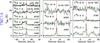 |
Fig. C.19 Observed 12CO, 13CO, and C18O transitions for TMC1A. |
Observed line intensities for TMC1A in all observed transitions.
Appendix C.20: TMC1
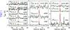 |
Fig. C.20 Observed 12CO, 13CO, and C18O transitions for TMC1. |
Observed line intensities for TMC1 in all observed transitions.
Appendix C.21: HH46
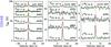 |
Fig. C.21 Observed 12CO, 13CO, and C18O transitions for HH46. |
Observed line intensities for HH46 in all observed transitions.
Appendix C.22: DK Cha
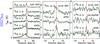 |
Fig. C.22 Observed 12CO, 13CO, and C18O transitions for DK Cha. |
Observed line intensities for DK Cha in all observed transitions.
Appendix C.23: GSS30IRS1
 |
Fig. C.23 Observed 12CO, 13CO, and C18O transitions for GSS30IRS1. |
Observed line intensities for GSS30IRS1 in all observed transitions.
Appendix C.24: Elias29
 |
Fig. C.24 Observed 12CO, 13CO, and C18O transitions for Elias29. |
Observed line intensities for Elias29 in all observed transitions.
Appendix C.25: Oph IRS63
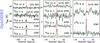 |
Fig. C.25 Observed 12CO, 13CO, and C18O transitions for Oph IRS63. |
Observed line intensities for OphIRS63 in all observed transitions.
Appendix C.26: RNO91
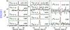 |
Fig. C.26 Observed 12CO, 13CO, and C18O transitions for RNO91. |
Observed line intensities for RNO91 in all observed transitions.
Appendix D: Herschel-HIFI observation IDs
Herschel obsids for related observations.
This publication is based on data acquired with the Atacama Pathfinder Experiment (APEX). APEX is a collaboration between the Max-Planck-Institut für Radioastronomie, the European Southern Observatory, and the Onsala Space Observatory.
The JCMT is operated by The Joint Astronomy Centre on behalf of the Science and Technology Facilities Council of the UK, The Netherlands Organisation for Scientific Research, and the National Research Council of Canada.
HIPE is a joint development by the Herschel Science Ground Segment Consortium, consisting of ESA, the NASA Herschel Science Center, and the HIFI, PACS and SPIRE consortia.
This research used the facilities of the Canadian Astronomy Data Centre operated by the National Research Council of Canada with the support of the Canadian Space Agency.
The only exception is IRAS 15398 where the targeted position is off source, see Kristensen et al. (2012).
The broad CO component is not necessarily the same physical component as seen in the broad H2O profiles; this point will be further discussed in Sect. 5.3.
Acknowledgments
The authors are grateful to the rest of the WISH team for stimulating discussions and to Joseph Mottram, Carolyn McCoey and the anonymous referee for valuable comments on the manuscript. They also thank the APEX, JCMT and Herschel staff as well as NL and MPIfR observers for carrying out the observations. Astrochemistry in Leiden is supported by The Netherlands Research School for Astronomy (NOVA), by a Spinoza grant and grant 614.001.008 from The Netherlands Organisation for Scientific Research (NWO), and by the European Community’s Seventh Framework Programme FP7/2007-2013 under grant agreement 238258 (LASSIE). The authors are grateful to many funding agencies and the HIFI-ICC staff who has been contributing for the construction of Herschel and HIFI for many years. HIFI has been designed and built by a consortium of institutes and university departments from across Europe, Canada and the United States under the leadership of SRON Netherlands Institute for Space Research, Groningen, The Netherlands and with major contributions from Germany, France and the US. Consortium members are: Canada: CSA, U.Waterloo; France: CESR, LAB, LERMA, IRAM; Germany: KOSMA, MPIfR, MPS; Ireland, NUI Maynooth; Italy: ASI, IFSI-INAF, Osservatorio Astrofisico di Arcetri- INAF; Netherlands: SRON, TUD; Poland: CAMK, CBK; Spain: Observatorio Astronómico Nacional (IGN), Centro de Astrobiología (CSIC-INTA). Sweden: Chalmers University of Technology – MC2, RSS GARD; Onsala Space Observatory; Swedish National Space Board, Stockholm University – Stockholm Observatory; Switzerland: ETH Zurich, FHNW; USA: Caltech, JPL, NHSC.Construction of CHAMP+ is a collaboration between the Max-Planck-Institut fur Radioastronomie Bonn, Germany; SRON Netherlands Institute for Space Research, Groningen, The Netherlands; The Netherlands Research School for Astronomy (NOVA); and the Kavli Institute of Nanoscience at Delft University of Technology, The Netherlands; with support from The Netherlands Organization for Scientific Research (NWO) grant 600.063.310.10.
References
- Alonso-Albi, T., Fuente, A., Crimier, N., et al. 2010, A&A, 518, A52 [NASA ADS] [CrossRef] [EDP Sciences] [Google Scholar]
- André, P., Ward-Thompson, D., & Barsony, M. 2000, Protostars & Planets IV, 59 [Google Scholar]
- Arce, H. G., Shepherd, D., Gueth, F., et al. 2007, Protostars and Planets V, 245 [Google Scholar]
- Bachiller, R., & Perez Gutierrez, M. 1997, ApJ, 487, L93 [NASA ADS] [CrossRef] [Google Scholar]
- Bachiller, R., Martin-Pintado, J., Tafalla, M., Cernicharo, J., & Lazareff, B. 1990, A&A, 231, 174 [NASA ADS] [Google Scholar]
- Bjerkeli, P., Liseau, R., Larsson, B., et al. 2012, A&A, 546, A29 [NASA ADS] [CrossRef] [EDP Sciences] [Google Scholar]
- Blake, G. A., Sandell, G., van Dishoeck, E. F., et al. 1995, ApJ, 441, 689 [Google Scholar]
- Bontemps, S., André, P., Terebey, S., & Cabrit, S. 1996, A&A, 311, 858 [Google Scholar]
- Bourke, T. L., Garay, G., Lehtinen, K. K., et al. 1997, ApJ, 476, 781 [NASA ADS] [CrossRef] [Google Scholar]
- Buckle, J. V., Hills, R. E., Smith, H., et al. 2009, MNRAS, 399, 1026 [NASA ADS] [CrossRef] [Google Scholar]
- Ceccarelli, C., Caselli, P., Herbst, E., Tielens, A. G. G. M., & Caux, E. 2007, Protostars and Planets V, 47 [Google Scholar]
- Chen, H., Myers, P. C., Ladd, E. F., & Wood, D. O. S. 1995, ApJ, 445, 377 [NASA ADS] [CrossRef] [Google Scholar]
- de Graauw, T., Helmich, F. P., Phillips, T. G., et al. 2010, A&A, 518, L6 [NASA ADS] [CrossRef] [EDP Sciences] [Google Scholar]
- Franklin, J., Snell, R. L., Kaufman, M. J., et al. 2008, ApJ, 674, 1015 [NASA ADS] [CrossRef] [Google Scholar]
- Fuchs, G. W., Cuppen, H. M., Ioppolo, S., et al. 2009, A&A, 505, 629 [NASA ADS] [CrossRef] [EDP Sciences] [Google Scholar]
- Fuente, A., Caselli, P., McCoey, C., et al. 2012, A&A, 540, A75 [NASA ADS] [CrossRef] [EDP Sciences] [Google Scholar]
- Fuller, G. A., & Ladd, E. F. 2002, ApJ, 573, 699 [NASA ADS] [CrossRef] [Google Scholar]
- Goicoechea, J. R., Cernicharo, J., Karska, A., et al. 2012, A&A, 548, A77 [NASA ADS] [CrossRef] [EDP Sciences] [Google Scholar]
- Goldsmith, P. F., & Langer, W. D. 1999, ApJ, 517, 209 [NASA ADS] [CrossRef] [Google Scholar]
- Green, J. D., Evans, II, N. J., Jørgensen, J. K., et al. 2013, ApJ, 770, 123 [NASA ADS] [CrossRef] [Google Scholar]
- Gregersen, E. M., Evans, II, N. J., Zhou, S., & Choi, M. 1997, ApJ, 484, 256 [NASA ADS] [CrossRef] [Google Scholar]
- Griffin, M. J., Abergel, A., Abreu, A., et al. 2010, A&A, 518, L3 [Google Scholar]
- Güsten, R., Baryshev, A., Bell, A., et al. 2008, in SPIE Conf. Ser., 7020 [Google Scholar]
- Harsono, D., Visser, R., Bruderer, S., et al. 2013, A&A, 555, A45 [NASA ADS] [CrossRef] [EDP Sciences] [Google Scholar]
- Hatchell, J., Richer, J. S., Fuller, G. A., et al. 2005, A&A, 440, 151 [NASA ADS] [CrossRef] [EDP Sciences] [Google Scholar]
- Hayashi, M., Hasegawa, T., Ohashi, N., & Sunada, K. 1994, ApJ, 426, 234 [NASA ADS] [CrossRef] [Google Scholar]
- Herczeg, G. J., Karska, A., Bruderer, S., et al. 2012, A&A, 540, A84 [NASA ADS] [CrossRef] [EDP Sciences] [Google Scholar]
- Hogerheijde, M. R., & van der Tak, F. F. S. 2000, A&A, 362, 697 [NASA ADS] [Google Scholar]
- Jørgensen, J. K., Schöier, F. L., & van Dishoeck, E. F. 2002, A&A, 389, 908 [NASA ADS] [CrossRef] [EDP Sciences] [Google Scholar]
- Jørgensen, J. K., Schöier, F. L., & van Dishoeck, E. F. 2004, A&A, 416, 603 [NASA ADS] [CrossRef] [EDP Sciences] [Google Scholar]
- Jørgensen, J. K., Schöier, F. L., & van Dishoeck, E. F. 2005a, A&A, 437, 501 [NASA ADS] [CrossRef] [EDP Sciences] [Google Scholar]
- Jørgensen, J. K., Schöier, F. L., & van Dishoeck, E. F. 2005b, A&A, 435, 177 [NASA ADS] [CrossRef] [EDP Sciences] [Google Scholar]
- Karska, A., Herczeg, G. J., van Dishoeck, E. F., et al. 2013, A&A, 552, A141 [NASA ADS] [CrossRef] [EDP Sciences] [Google Scholar]
- Kasemann, C., Güsten, R., Heyminck, S., et al. 2006, in SPIE Conf. Ser., 6275 [Google Scholar]
- Kristensen, L. E., van Dishoeck, E. F., Tafalla, M., et al. 2011, A&A, 531, L1 [Google Scholar]
- Kristensen, L. E., van Dishoeck, E. F., Bergin, E. A., et al. 2012, A&A, 542, A8 [NASA ADS] [CrossRef] [EDP Sciences] [Google Scholar]
- Kutner, M. L., & Ulich, B. L. 1981, ApJ, 250, 341 [NASA ADS] [CrossRef] [Google Scholar]
- Lacy, J. H., Knacke, R., Geballe, T. R., & Tokunaga, A. T. 1994, ApJ, 428, L69 [NASA ADS] [CrossRef] [Google Scholar]
- Lada, C. J. 1999, in NATO ASIC Proc. 540: The Origin of Stars and Planetary Systems, eds. C. J. Lada, & N. D. Kylafis, 143 [Google Scholar]
- Langer, W. D., & Penzias, A. A. 1990, ApJ, 357, 477 [NASA ADS] [CrossRef] [Google Scholar]
- Liseau, R., Goldsmith, P. F., Larsson, B., et al. 2012, A&A, 541, A73 [NASA ADS] [CrossRef] [EDP Sciences] [Google Scholar]
- Loren, R. B. 1989, ApJ, 338, 902 [NASA ADS] [CrossRef] [Google Scholar]
- Manoj, P., Watson, D. M., Neufeld, D. A., et al. 2013, ApJ, 763, 83 [NASA ADS] [CrossRef] [Google Scholar]
- Müller, H. S. P., Schlöder, F., Stutzki, J., & Winnewisser, G. 2005, J. Mol. Struct., 742, 215 [NASA ADS] [CrossRef] [Google Scholar]
- Myers, P. C., & Ladd, E. F. 1993, ApJ, 413, L47 [NASA ADS] [CrossRef] [Google Scholar]
- Myers, P. C., Evans, II, N. J., & Ohashi, N. 2000, Protostars and Planets IV, 217 [Google Scholar]
- Ossenkopf, V., & Henning, T. 1994, A&A, 291, 943 [NASA ADS] [Google Scholar]
- Ott, S. 2010, in Astronomical Data Analysis Software and Systems XIX, eds. Y. Mizumoto, K.-I. Morita, & M. Ohishi, ASP Conf. Ser., 434, 139 [Google Scholar]
- Pickett, H. M., Poynter, R. L., Cohen, E. A., et al. 2010, J. Quant. Spect. Radiat. Trans., 111, 1617 [Google Scholar]
- Pilbratt, G. L., Riedinger, J. R., Passvogel, T., et al. 2010, A&A, 518, L1 [CrossRef] [EDP Sciences] [Google Scholar]
- Plume, R., Bergin, E. A., Phillips, T. G., et al. 2012, ApJ, 744, 28 [NASA ADS] [CrossRef] [Google Scholar]
- Poglitsch, A., Waelkens, C., Geis, N., et al. 2010, A&A, 518, L2 [NASA ADS] [CrossRef] [EDP Sciences] [Google Scholar]
- Robitaille, T. P., Whitney, B. A., Indebetouw, R., Wood, K., & Denzmore, P. 2006, ApJS, 167, 256 [NASA ADS] [CrossRef] [Google Scholar]
- Roelfsema, P. R., Helmich, F. P., Teyssier, D., et al. 2012, A&A, 537, A17 [NASA ADS] [CrossRef] [EDP Sciences] [Google Scholar]
- San José-García, I., Mottram, J. C., Kristensen, L. E., et al. 2013, A&A, 553, A125 [NASA ADS] [CrossRef] [EDP Sciences] [Google Scholar]
- Santangelo, G., Nisini, B., Giannini, T., et al. 2012, A&A, 538, A45 [NASA ADS] [CrossRef] [EDP Sciences] [Google Scholar]
- Schöier, F. L., van der Tak, F. F. S., van Dishoeck, E. F., & Black, J. H. 2005, A&A, 432, 369 [NASA ADS] [CrossRef] [EDP Sciences] [Google Scholar]
- Shirley, Y. L., Evans, II, N. J., Rawlings, J. M. C., & Gregersen, E. M. 2000, ApJS, 131, 249 [NASA ADS] [CrossRef] [Google Scholar]
- Spaans, M., Hogerheijde, M. R., Mundy, L. G., & van Dishoeck, E. F. 1995, ApJ, 455, L167 [NASA ADS] [Google Scholar]
- Tachihara, K., Onishi, T., Mizuno, A., & Fukui, Y. 2002, A&A, 385, 909 [NASA ADS] [CrossRef] [EDP Sciences] [Google Scholar]
- Tafalla, M., Santiago-García, J., Hacar, A., & Bachiller, R. 2010, A&A, 522, A91 [NASA ADS] [CrossRef] [EDP Sciences] [Google Scholar]
- Tafalla, M., Liseau, R., Nisini, B., et al. 2013, A&A, 551, A116 [NASA ADS] [CrossRef] [EDP Sciences] [Google Scholar]
- van der Tak, F. F. S., Black, J. H., Schöier, F. L., Jansen, D. J., & van Dishoeck, E. F. 2007, A&A, 468, 627 [NASA ADS] [CrossRef] [EDP Sciences] [Google Scholar]
- van Dishoeck, E. F., & Blake, G. A. 1998, ARA&A, 36, 317 [NASA ADS] [CrossRef] [Google Scholar]
- van Dishoeck, E. F., Kristensen, L. E., Benz, A. O., et al. 2011, PASP, 123, 138 [NASA ADS] [CrossRef] [Google Scholar]
- van Kempen, T. A., Hogerheijde, M. R., van Dishoeck, E. F., et al. 2006, A&A, 454, L75 [NASA ADS] [CrossRef] [EDP Sciences] [Google Scholar]
- van Kempen, T. A., van Dishoeck, E. F., Güsten, R., et al. 2009a, A&A, 507, 1425 [NASA ADS] [CrossRef] [EDP Sciences] [Google Scholar]
- van Kempen, T. A., van Dishoeck, E. F., Güsten, R., et al. 2009b, A&A, 501, 633 [NASA ADS] [CrossRef] [EDP Sciences] [Google Scholar]
- van Kempen, T. A., van Dishoeck, E. F., Hogerheijde, M. R., & Güsten, R. 2009c, A&A, 508, 259 [Google Scholar]
- van Kempen, T. A., van Dishoeck, E. F., Salter, D. M., et al. 2009d, A&A, 498, 167 [NASA ADS] [CrossRef] [EDP Sciences] [Google Scholar]
- van Kempen, T. A., Kristensen, L. E., Herczeg, G. J., et al. 2010, A&A, 518, L121 [NASA ADS] [CrossRef] [EDP Sciences] [Google Scholar]
- Vasta, M., Codella, C., Lorenzani, A., et al. 2012, A&A, 537, A98 [NASA ADS] [CrossRef] [EDP Sciences] [Google Scholar]
- Visser, R., & Dullemond, C. P. 2010, A&A, 519, A28 [NASA ADS] [CrossRef] [EDP Sciences] [Google Scholar]
- Visser, R., van Dishoeck, E. F., Doty, S. D., & Dullemond, C. P. 2009, A&A, 495, 881 [NASA ADS] [CrossRef] [EDP Sciences] [Google Scholar]
- Visser, R., Kristensen, L. E., Bruderer, S., et al. 2012, A&A, 537, A55 [NASA ADS] [CrossRef] [EDP Sciences] [Google Scholar]
- Vladilo, G., Centurion, M., & Cassola, C. 1993, A&A, 273, 239 [NASA ADS] [Google Scholar]
- Wilson, T. L., & Rood, R. 1994, ARA&A, 32, 191 [NASA ADS] [CrossRef] [Google Scholar]
- Yang, B., Stancil, P. C., Balakrishnan, N., & Forrey, R. C. 2010, ApJ, 718, 1062 [NASA ADS] [CrossRef] [Google Scholar]
- Yıldız, U. A., van Dishoeck, E. F., Kristensen, L. E., et al. 2010, A&A, 521, L40 [Google Scholar]
- Yıldız, U. A., Kristensen, L. E., van Dishoeck, E. F., et al. 2012, A&A, 542, A86 [NASA ADS] [CrossRef] [EDP Sciences] [Google Scholar]
- Young, C. H., & Evans, II, N. J. 2005, ApJ, 627, 293 [NASA ADS] [CrossRef] [Google Scholar]
Appendix A: CO 10–9/3–2 spectra
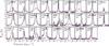 |
Fig. A.1 Zoom-in spectra of the line wings of 12CO 3–2 (black) and 12CO 10–9 (magenta) overplotted for each source. The spectra are multiplied by a constant factor indicated in the figure in order to show the line wings in more detail. They have been rebinned to 0.6–1 km s-1, to enhance signal-to-noise. |
Appendix B: Observations matrix
Observed sources and lines.
All Tables
Relative fractions of integrated intensities calculated for broad and narrow components in 12CO 10–9 lines.
Median rotational temperatures and colum densities of Class 0 and Class I sources calculated from 12CO, 13CO and C18O.
All Figures
|
Fig. 1 On source CO spectra convolved to a ~20′′ beam. From left to right: 12CO 3–2, 10–9, 13CO 10–9, C18O 9–8, 5–4 and 10–9, respectively. Only the CO 3–2 lines are observed with the JCMT, the rest of the data are from Herschel-HIFI. The spectra are plotted by shifting the source velocity (Vlsr) to 0 km s-1 (actual source velocities are given in Table 4). The lines are shifted vertically. Intensity scale of some sources is multiplied by a constant value for easy viewing and marked if different from 1. The top half of the figure shows the Class 0 sources whereas the bottom part displays the Class I sources. The right-most column displays the C18O 5–4 and C18O 10–9 lines for the Class 0 sources only. The latter lines are very close to the H2O 312–303 line resulting in an intensity rise on the blue side of the spectrum in some sources. |
| In the text | |
|
Fig. 2 Gaussian decomposition of the 12CO 10–9 profile toward four sources. The profile toward two sources, L1527 and IRAS 4A, can be decomposed into a single Gaussian, whereas SMM3, IRAS 4B and all the remaining sources in the sample require two components (decomposition shown with the dashed red fit). |
| In the text | |
|
Fig. 3 Relative fraction of the integrated intensity of the narrow and broad components for each source. The 12CO 10–9 profile decomposition is given in San José-García et al. (2013). Yellow regions indicate the broad component fraction and black the narrow component fractions. The red dashed line divides the Class 0 (left) and Class I (right) sources. |
| In the text | |
|
Fig. 4 Composite H2O 110–101, CO 10–9 and CO 3–2 spectra of Class 0 and Class I sources averaged in order to compare the line profiles of two types of sources. All spectra are rescaled to a common distance of 200 pc, shifted to the central 0 km s-1 velocity, rebinned to a 0.3 km s-1 velocity resolution. The CO spectra refer to a 20′′ beam, the H2O spectra to a 40′′ beam. The red spectra overlaid on top of the 12CO 10–9 are obtained by normalizing all the spectra to a common peak temperature first and then averaging them. |
| In the text | |
|
Fig. 5 12CO 10–9 spectra of L1448 mm and BHR71, where bullet structures are shown. The green lines indicates the baseline and the red lines represent the Gaussian fits of the line profiles. Fit parameters are given in Table 3. |
| In the text | |
|
Fig. 6 Rotational diagrams for 12CO lines using the integrated intensities. All data are convolved to a 20″ beam and each plot shows the best single temperature fit to the observed transitions (see also Table 5). Left panel (red): Class 0 sources; right panel (blue): Class I sources. |
| In the text | |
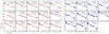 |
Fig. 7 Same as Fig. 6 but for 13CO lines. |
| In the text | |
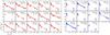 |
Fig. 8 Same as Fig. 6 but for C18O lines. |
| In the text | |
|
Fig. 9 Distribution of rotation temperatures (Trot) calculated from 12CO and 13CO line observations. The median temperatures are listed in Table 6. |
| In the text | |
|
Fig. 10 12CO spectral line energy distribution (SLED) for the observed transitions. All of the fluxes are normalized to their own CO 3–2 flux for Class 0 (left) and Class I (right) sources separately. The beams are ~20′′ beam. The thick lines are the median values of each transitions. |
| In the text | |
|
Fig. 11 Two temperature components fitted for selected sources to the 12CO lines, from 2–1 to 7–6 (cold), from 7–6 to 10–9 (warm), and 2–1 to 10–9 (global). |
| In the text | |
|
Fig. 12 Rotational temperatures calculated channel by channel for 12CO. Each spectrum is shifted to Vlsr = 0 km s-1 and rebinned to 3 km s-1 velocity resolution. |
| In the text | |
|
Fig. 13 Ratios of the CO 10–9/3–2 line wings for 14 protostars as function of velocity offset from the central emission. Spectra are shifted to Vlsr = 0 km s-1. The wings start at ±2.5 km s-1 from Vlsr in order to prevent adding the central self-absorption feature in the CO 3–2 lines. |
| In the text | |
|
Fig. 14 Model CO 10–9/3–2 line intensity ratios as function of temperature and density, obtained for a CO column density of 1016 cm-2 with line-widths of 10 km s-1, representative of the observed CO intensity and line width. Note that the bars are the ranges of lower and upper limits as seen from the observations in Fig. 13. Red markers are for Class 0 and blue markers are for Class I sources. Blue wing ratios are indicated with triangles and red wing ratios have square symbols. Thick magenta and black lines indicate the ratios from the composite spectra for Class 0 and Class I sources, respectively. Vertical dashed lines indicate the limits for ncr for CO 3–2 (brown) and CO 10–9 (green). In the relevant density range, higher ratios are indicative of higher kinetic temperatures. |
| In the text | |
|
Fig. 15 From top to bottom, 12CO 10–9, 13CO 10–9, and C18O 3–2 integrated intensity W normalized at 200 pc are plotted against various physical properties: envelope mass at 10 K radius, Menv; bolometric temperature, Tbol; and bolometric luminosity, Lbol. Green lines are the best fit to the data points and r values in each of the plots are Pearson correlation coefficient. |
| In the text | |
|
Fig. 16 Calculated rotational temperatures, Trot, plotted Menv, Tbol, and Lbol, for 12CO (top), 13CO (middle), C18O lines (bottom). The median excitation temperatures of ~70 K, 48 K and 37 K for 12CO, 13CO and C18O, respectively, are indicated with the green dashed lines. Typical error bar for each of the Trot values is shown in the upper left plot, represented in black circle data point. In the C18O plots, blue arrows indicate the upper limits for a number of sources. These figures are compared with disk evolution models of Harsono et al. (2013, magenta solid lines), which represents all three models discussed in the text. Magenta arrows also show the direction of time. The figures show that the excitation temperature does not change with the increasing luminosity, envelope mass or density, confirming that Class 0 and I sources have similar excitation conditions. |
| In the text | |
|
Fig. 17 Blue and red line wing ratios of CO 10–9/3–2 (top panel), H2O 110–101/CO 10–9 (middle panel), and H2O 110–101/CO 3–2 (bottom panel) for the composite Class 0 and Class I source spectra. The H2O/CO 10–9 and H2O/CO 3–2 ratios are a factor of two lower than shown in Fig. 4 due to the beam size difference of 20″ (CO 10–9 lines) to 40″ (H2O 110–101 lines). |
| In the text | |
|
Fig. 18 Constant abundance profiles are fitted to the lower-J C18O 3–2 are shown as function of Lbol and Menv. Green lines are the best fit to the data points and r values in each of the plots are Pearson correlation coefficient. |
| In the text | |
|
Fig. 19 Cumulative intensity I/Itot for various C18O lines as function of envelope radius (as indicated by the temperature To) with the dust opacity included (solid curves), and dust opacity off (dashed curves). The dash-dotted lines indicates the fractions of 50 and 80%, respectively. |
| In the text | |
|
Fig. 20 Dust optical depth at 1 THz as function of envelope radius and temperature. Horizontal dashed lines indicate the τ = 1 and τ = 0.1 values whereas vertical dash-dotted lines are radii, where the temperatures are between 40 K and 60 K. |
| In the text | |
|
Fig. C.1 Observed 12CO, 13CO, and C18O transitions for L1448MM. |
| In the text | |
|
Fig. C.2 Observed 12CO, 13CO, and C18O transitions for IRAS 2A. |
| In the text | |
|
Fig. C.3 Observed 12CO, 13CO, and C18O transitions for IRAS 4A. |
| In the text | |
|
Fig. C.4 Observed 12CO, 13CO, and C18O transitions for IRAS 4B. |
| In the text | |
|
Fig. C.5 Observed 12CO, 13CO, and C18O transitions for L1527. |
| In the text | |
|
Fig. C.6 Observed 12CO, 13CO, and C18O transitions for Ced110-IRS4. |
| In the text | |
|
Fig. C.7 Observed 12CO, 13CO, and C18O transitions for BHR71. |
| In the text | |
|
Fig. C.8 Observed 12CO, 13CO, and C18O transitions for IRAS15398. |
| In the text | |
|
Fig. C.9 Observed 12CO, 13CO, and C18O transitions for L483 mm. |
| In the text | |
|
Fig. C.10 Observed 12CO, 13CO, and C18O transitions for SerSMM1. |
| In the text | |
|
Fig. C.11 Observed 12CO, 13CO, and C18O transitions for SerSMM4. |
| In the text | |
|
Fig. C.12 Observed 12CO, 13CO, and C18O transitions for SerSMM3. |
| In the text | |
|
Fig. C.13 Observed 12CO, 13CO, and C18O transitions for L723 mm. |
| In the text | |
|
Fig. C.14 Observed 12CO, 13CO, and C18O transitions for B335. |
| In the text | |
|
Fig. C.15 Observed 12CO, 13CO, and C18O transitions for L1157. |
| In the text | |
|
Fig. C.16 Observed 12CO, 13CO, and C18O transitions for L1489. |
| In the text | |
|
Fig. C.17 Observed 12CO, 13CO, and C18O transitions for L1551IRS5. |
| In the text | |
|
Fig. C.18 Observed 12CO, 13CO, and C18O transitions for TMR1. |
| In the text | |
|
Fig. C.19 Observed 12CO, 13CO, and C18O transitions for TMC1A. |
| In the text | |
|
Fig. C.20 Observed 12CO, 13CO, and C18O transitions for TMC1. |
| In the text | |
|
Fig. C.21 Observed 12CO, 13CO, and C18O transitions for HH46. |
| In the text | |
|
Fig. C.22 Observed 12CO, 13CO, and C18O transitions for DK Cha. |
| In the text | |
|
Fig. C.23 Observed 12CO, 13CO, and C18O transitions for GSS30IRS1. |
| In the text | |
|
Fig. C.24 Observed 12CO, 13CO, and C18O transitions for Elias29. |
| In the text | |
|
Fig. C.25 Observed 12CO, 13CO, and C18O transitions for Oph IRS63. |
| In the text | |
|
Fig. C.26 Observed 12CO, 13CO, and C18O transitions for RNO91. |
| In the text | |
|
Fig. A.1 Zoom-in spectra of the line wings of 12CO 3–2 (black) and 12CO 10–9 (magenta) overplotted for each source. The spectra are multiplied by a constant factor indicated in the figure in order to show the line wings in more detail. They have been rebinned to 0.6–1 km s-1, to enhance signal-to-noise. |
| In the text | |
Current usage metrics show cumulative count of Article Views (full-text article views including HTML views, PDF and ePub downloads, according to the available data) and Abstracts Views on Vision4Press platform.
Data correspond to usage on the plateform after 2015. The current usage metrics is available 48-96 hours after online publication and is updated daily on week days.
Initial download of the metrics may take a while.