| Issue |
A&A
Volume 556, August 2013
|
|
|---|---|---|
| Article Number | A97 | |
| Number of page(s) | 11 | |
| Section | Extragalactic astronomy | |
| DOI | https://doi.org/10.1051/0004-6361/201220832 | |
| Published online | 02 August 2013 | |
Towards equation of state of dark energy from quasar monitoring: Reverberation strategy
1
Nicolaus Copernicus Astronomical Center, Bartycka 18,
00-716
Warsaw,
Poland
e-mail: This email address is being protected from spambots. You need JavaScript enabled to view it.
2
Adam Mickiewicz University Observatory,
ul. Sloneczna 36, 60-286
Poznan,
Poland
3
Astrophysics, Cosmology and Gravity Centre, Department of
Astronomy, University of Cape Town, Private Bag X3, 7701
Rondebosch, Republic of
South Africa
Received: 2 December 2012
Accepted: 25 May 2013
Abstract
Context. High-redshift quasars can be used to constrain the equation of state of dark energy. They can serve as a complementary tool to supernovae Type Ia, especially at z > 1.
Aims. The method is based on the determination of the size of the broad line region (BLR) from the emission line delay, the determination of the absolute monochromatic luminosity either from the observed statistical relation or from a model of the formation of the BLR, and the determination of the observed monochromatic flux from photometry. This allows the luminosity distance to a quasar to be obtained, independently from its redshift. The accuracy of the measurements is, however, a key issue.
Methods. We modeled the expected accuracy of the measurements by creating artificial quasar monochromatic lightcurves and responses from the BLR under various assumptions about the variability of a quasar, BLR extension, distribution of the measurements in time, accuracy of the measurements, and the intrinsic line variability.
Results. We show that the five-year monitoring of a single quasar based on the Mg II line should give an accuracy of 0.06−0.32 mag in the distance modulus which will allow new constraints to be put on the expansion rate of the Universe at high redshifts. Successful monitoring of higher redshift quasars based on C IV lines requires proper selection of the objects to avoid sources with much higher levels of the intrinsic variability of C IV compared to Mg II.
Key words: quasars: emission lines / cosmological parameters / dark energy / accretion, accretion disks / black hole physics
© ESO, 2013
1. Introduction
The key issue of present day cosmology is determining the properties of the dark energy that drives the accelerated expansion of the Universe (for a review, see Frieman et al. 2008; Amendola & Tsuikawa 2010; Li et al. 2011; Mattarese et al. 2011). The need for the cosmological constant was already recognized in the early 1980s (e.g., Peebles 1984), but the arguments in favor accumulated slowly. The situation started to change after the release of the COBE cosmic microwave background (CMB) measurements, particularly when combined with other constraints coming from large structure formation. For example, Kofman et al. (1993) estimated that ΩΛ ~ 0.3−0.4. The convincing evidence for Λ > 0 came with the observations of supernovae Ia (SNe Ia; Riess et al. 1998; Perlmutter et al. 1998), which lead to the emergence of the standard cosmological model known as lambda cold dark matter (ΛCDM). There has been considerable quantitative progress since that time with the emergence of precision cosmology. The presence of dark energy is now well supported observationally, and most of the results are still consistent with its simplest interpretation as a cosmological constant. However, a number of dark energy models have been proposed, giving more general predictions for the equation of state, P = wρc2, than the simple cosmological constant, which corresponds to w = −1. An example of a more complicated model of this nature is the quintessence model, where w is constant in time and lies in the range −1 < w < −1/3, or the phantom dark energy model with w < −1. In even more general model w can change with time, and equivalently, with redshift (e.g., Chevallier & Polarski 2001).
The most recent results for z ~ 1 supernovae of Suzuki et al. (2012) imply ΩΛ = 0.729 ± 0.014 for a ΛCDM model, and  (68% confidence level) for a flat w cold dark matter (wCDM) model. Similar numbers have been obtained based on CMB measurements: the Wilkinson microwave anisotropy probe (WMAP) nine-year data analysis gives ΩΛ = 0.721 ± 0.025 (Hinshaw et al. 2012), whereas Planck 2013 results point to a somewhat lower value (ΩΛ = 0.686 ± 0.020; Planck Collaboration 2013, Table 2). Both experiments show additionally that the simplest ΛCDM model with w = −1 is a very good fit to the data, although various degeneracies do not allow other dark energy equations of state to be excluded. Additional constraints on the expansion history of the Universe come from the large-scale structure studies, for instance via baryon acoustic oscillations (Eisenstain et al. 2005; Sanchez et al. 2012) or redshift-space distortions (Guzzo et al. 2008). New methods are constantly being suggested, like those based on the weak lensing of galaxies (statistical approach: Jain & Taylor 2003, individual sources: Biesiada & Piorkowska 2009), combined X-ray emission and the Sunyaev-Zel’dovich effect in galaxy clusters (see Benson et al. 2013 and the references therein), gamma-ray bursts (e.g., Dainotti et al. 2011) and standard sirens in gravitational waves (suplemented with redshift, Schutz 1986; or without it, Seto et al. 2001). Combining these methods allows for independent checks of the validity of the standard cosmological model. However, the dark energy equation of state and its redshift evolution cannot be well constrained from low-redshift and CMB data only: one needs to directly probe the expansion rate at z ≳ 1 to effectively study the time evolution of w. At these redshifts, however, SNe Ia are very difficult to observe, because of a considerable shift of their spectra towards the infrared and cosmological dimming (∝ (1 + z)4).
Watson et al. (2011) proposed that active galactic nuclei (AGN) can also be used as probes of dark energy, complementary to the study done with other methods. The basic idea is the following. The absolute size of the broad line region (BLR) in AGN can be measured from the time delay between the variable continuum emission from the nucleus and the emission lines in the optical/UV band (e.g., Blandford & McKee 1982; Peterson 1993; Sergeev et al. 1994; Wandel et al. 1999). This reverberation technique based on the Hβ line was succesfully used for low-redshift objects (up to z = 0.292; Kaspi et al. 2000; Bentz et al. 2009a,b). The size of the BLR is related to the absolute value of the source monochromatic luminosity. This was found observationally (Kaspi et al. 2000; Peterson et al. 2004; Bentz et al. 2009a), but the relation was later theoretically explained by Czerny & Hryniewicz (2011) as corresponding to the formation of the inner radius of BLR at a fixed temperature of 1000 K in all sources, independently from the black hole mass and accretion rate. This result points toward the important role of dust in the accretion disk atmosphere in the formation of BLR, connecting it with the dust sublimation temperature. Having the absolute value of the monochromatic luminosity, and measuring the observed monochromatic luminosity, we can determine the luminosity distance to the source. Summarizing, the measurement of the observed monochromatic flux and of the time delay between the continuum and a BLR emission line for a number of sources allows the diagram of the luminosity distance as a function of redshift to be constructed, and to test the cosmological models.
The use of an independent tracer of the dark energy is important. Various methods are being used or will be used to trace the dark energy, but each of them can have a certain bias. Supernovae luminosity may be subject to systematic cosmological evolution, owing to the evolution of the chemical content of the Universe. Quasars show roughly solar or slightly super-solar metallicity, even to redshifts of a few (e.g., Dietrich et al. 2003a,b; Simon & Hamann 2010; De Rosa et al. 2011; Gall et al. 2011), probably because to the correlated evolution of starburst and quasar activity. Therefore, the relation between the size of the BLR and monochromatic luminosity, reflecting dust properties, should not contain strong evolutionary trends with the redshift. Other methods, like galaxy clusters, weak gravitational lensing, and galaxy angular clustering (baryon acoustic oscillations) can also contain some bias since the clusters are not spherically symmetric and relaxed, and galaxy clustering may be the subject of magnification bias. If numerous independent methods are used, the results will be more reliable.
We have recently started an observational campaign with the Southern African Large Telescope (SALT) to collect data for reverberation studies of a sample of seven objects. We are planning to use the low-ionization line of Mg II 2798 Å, which is suitable for studies of objects in the redshift range from 0.9 to 1.4. So far only a few authors have claimed the measurement of the delay in Seyfert galaxies using Mg II or C IV line in HST or IUE data (Clavel et al. 1991 for NGC 5548, z = 0.017175 using Mg II and C IV; Reichert et al. 1994 for NGC 3783, z = 0.00973, using Mg II and C IV; Wang et al. 1997 and O’Brien et al. 1998 for 3C 390.3, z = 0.0561, using C IV; Peterson & Wandel 1999 for NGC 5548, z = 0.017175, using C IV; Peterson et al. 2004 for Fairall 9, z = 0.047016, using Mg II; Metzroth et al. 2006 for NGC 4151, z = 0.003319, using C IV and Mg II). For higher redshift objects Chelouche et al. (2012) were able to measure the delay for MACHO 13.6805.324, z = 1.72, from a photometric method, but in this case the measurement probably represents the response of the iron pseudo-continuum. Woo (2008) showed that using the Mg II line is an attractive possibility, but the two-year monitoring program was too short to attempt any delay measurement. Reverberation studies of even higher redshift quasars, based on the C IV 1549 Å line, were done with the Hobby-Eberly Telescope (HET) by Kaspi et al. (2007), but the authors were generally not successful in the measurement of the time delays, with a tentative delay measurement of 595 days for one object (S5 0836+71) out of six. Therefore, in this paper we perform a detailed analysis of the requirements for a successful monitoring program.
2. Method
Active galactic nuclei are highly variable in all energy bands (for a review, see Ulrich et al. 1997), including the optical band (e.g., Matthews & Sandage 1963; Hawkins 1983; Barbieri et al. 1988; Cristiani et al. 1996; Van den Berk et al. 2004; Bauer et al. 2009; MacLoad et al. 2012). Although the best studies were done in the X-ray band, there were also several attempts to describe quantitatively the character of the optical variability. The power density spectra (PDS) in the optical band for NGC 4151 were constructed by Terebizh et al. (1989) and by Czerny et al. (2003) in the long timescale, and by Edelson et al. (1996) in the short timescale; for NGC 5548 by Czerny et al. (1999).
Our idea here was to create simulated datasets of a fiducial high-redshift quasar to estimate the role of various parameters of an observational campaign (e.g., number and separations of observations, duration of the campaign) and expected quality of data, in the accuracy of the determined reverberation time delay. This should help to develop the optimum strategy of a reverberation studies campaign.
We used the Timmer & König (1995) algorithm to generate an artificial continuum lightcurve of a quasar based on the assumed shape of the PDS. We then exponentiated the resulting lightcurve, following Uttley et al. (2005), since this reproduces the log-normal distribution characteristic for high-energy lightcurves of accreting sources. We assume that the PDS has a shape of a doubly-broken power law, although the long-term variability is highly uncertain, but this allows us to test whether there are any effects of the power leak toward shorter frequencies. We fix the longest frequency slope at zero, while the two remaining slopes, s1 and s2, and the break frequencies, f1 and f2, are in general the free parameters of the simulations. We expect that they are mostly affected by the value of the black hole mass of the monitored quasar, since in the X-ray band the black hole mass is the key parameter of the PDS (Hayashida et al. 1998; Czerny et al. 2001; Papadakis 2004, Zhou et al. 2010; Ponti et al. 2012), although the effect of the Eddington ratio and/or spectral state is an issue (e.g., McHardy et al. 2006; Nikolajuk et al. 2009). We fix these parameters at s1 = 1.2, s2 = 2.5, f1 = 0.012 yr-1, and f2 = 0.18 yr-1. These values were estimated from the optical PDS of NGC 5548 (the intermediate slope s1 and the break frequencies f1 and f2), while the high-frequency slope s2 was taken from the Kepler quasars monitoring campaign, after correcting the slope for the subtraction of the linear trend (Mushotzky et al. 2011). The break frequencies were then scaled to a higher expected black hole mass, and for the redshift. The overall dimensionless amplitude of the PDF is also a model parameter, but again in most simulations it was fixed at 0.1 and 0.3, which correspond to the dimensionless dispersion in the infinite photometric lightcurve (i.e., of duration above 1000 yr) without any measurement error of 0.32 and 1.61, correspondingly. The created lightcurves have the total standard length of 30 years and are densly spaced (1 day).
Next we modeled the response of the BLR (meant to be represented by the Mg II 2798 Å line) to the variability of the continuum. In the simplest approach, the line lightcurve is created by convolving the continuum lightcurve with a Gaussian kernel. The center of the Gaussian represents the line delay after the continuum, which is a free parameter of the model, and is on the order of a few hundred days. The Gaussian width models the smearing of the response resulting from the finite extension of the BLR. Most of the reprocessing was done by the BLR part located on the far side of the black hole since the clouds on the side toward the observer are dark and so do not emit efficiently. Therefore, in most computations we assumed the Gaussian width on the order of 10 percent of the time delay, since such parameters recover well the measured accuracy of the time delay for NGC 5548. However, we also experimented with other values of the Gaussian width and with more complex BLR response.
Obviously, the photometric and spectroscopic monitoring with the SALT telescope cannot be done with 1-day spacing, so in the next step we selected observational points from the two light curves, assuming a realistic observational pattern and also simulating the measurement errors. In most cases we assume that the object cannot be observed for about three months every year (because it is out of the observational window of SALT), and the gap is the same for photometric and spectroscopic lightcurves. For photometric monitoring we assume that the object will be observed roughly every two weeks, with random dispersion of 3 days. For spectroscopic measurements, we assume five SALT observations every year, with random dispersion of 14 days. We can, of course, vary these parameters as well.
Finally, we had to account for possible uncertainties of both the spectroscopic and photometric measurements. Therefore, the value of the lightcurve at each observational point was replaced with a random value obtained from a Gaussian distribution with the mean equal to this value and the dispersion corresponding to the assumed 1σ error. The errors for the line measurement are generally assumed to be larger than the errors of the photometric measurements. As a default, we used the conservative estimate of 5% accuracy in photometry and 10% accuracy in spectroscopy.
Having the two curves, we then measured the time delay of the spectroscopic lightcurve compared to the photometric, for example using the interpolated cross-correlation function (ICCF) as is usually done for the real data (e.g., Gaskell & Peterson 1987). We interpolated the spectroscopic measurements to the dates of the photometric measurements, and we used the maximum of the ICCM to determine the delay. To determine the expected accuracy of the measurements, for each set of all the other parameters we analyzed 1000 random realizations of the process, and we created the histogram of the measured delays. The comparison of this histogram to the assumed delay characterizes the expected quality of the observational campaign. In particular, we used the median of the histogram to gave the best value of the delay, and for the dispersion we give the dispersion around the known expected value. In addition we gave the spread, defined as a half range between the 1−0.158 and 0.158 quantiles of the histogram. For the Gaussian distribution it would correspond to a 1σ error. We also experimented with alternative methods to measure time delay. The whole procedure should mimic well the actual reverberation measurements performed for numerous less distant sources (e.g., Kaspi et al. 2000; Peterson et al. 2002; Bentz et al. 2009a,b; Denney et al. 2009, 2010; Walsh et al. 2009; Barth et al. 2011; Stalin et al. 2011; Dietrich et al. 2012; Grier et al. 2012a,b).
We tested the method using the past monitoring of NGC 5548. The optical power spectrum for this source was described as a power law with two breaks, with the slopes as above but lower frequency breaks (f1 = 0.11 yr-1 and f2 = 3.6 yr-1). We assumed 0.04 for the dimensionless level of variability. For the observational setup, we considered the sparse monitoring described by Peterson et al. (2002) and the dense short Lick monitoring presented by Walsh et al. (2009) and Bentz et al. (2009b). In the case of the first monitoring, we used the setup for Year 8 (1996), with the measured delay of 15.3 days. We took 5% and 4% for the photometry and spectroscopy errors, respectively. The computations returned the delay measurement of 15.0 ± 1.9 days with the rms of 8.5% and 10.2% for photometry and spectroscopy, close to observed values (15% and 11%, respectively). The second monitoring lasted for 68 days, with 51 line measurements; we assumed the measurement errors of 2% and 6% for photometry and spectroscopy, representative for this monitoring, and we assumed the same overall variability normalization as before, but much shorter delay (4.2 days; the source was then in a very low state). We recovered the delay of 4.2 ± 1.8 days, with Fvar in the line and in the continuum of 8.5% 5.4%, again similar to the observed values.
Parameters of the models and the accuracy of the delay recovery for variability amplitude 0.1, assumed delay 660 days.
Parameters of the models and the accuracy of the delay recovery for variability amplitude 0.3, assumed delay 660 days.
With our Monte Carlo approach we were then able to study which elements of the campaign are the most important ones and where there are possibilities for an improvement. These we hope will be of significant help in planning an observational project that will last about five years.
3. Results
We modeled the expected accuracy of the measurement of the emission line delay against the continuum for a single-object (high-redshift quasar) monitoring. The problem is important because the variability of AGN are of a red-noise type, with a broad range of timescales and a strong contributions from the timescales that are much longer than the observed lightcurves. The Monte Carlo approach is effective in assessing the likely results as well as possible caveats since in the real monitoring we have to work with just one realization of the process.
The basic model (hereafter model A) was adjusted to our ongoing observational campaign. The feasibility study was done for a quasar Q 2113-4538 (z = 0.946). The high redshift of the source ensures that the Mg II 2798 Å line is within the spectroscopy frame. The quasar comes from the Large Bright Quasar Sample (LBQS; e.g., Hewett et al. 1995), the black hole mass in this object was estimated to be 1.5 × 10⁹ M⊙ (Vestergaardt & Osmer 2009), and the expected time delay of the Mg II line (from the Kong et al. 2006 formula) is 660 days, if the additional increase due to the redshift is included. The spectroscopy was with the SALT and the source is visible for about nine months. We plan to perform five observations per year and three observations have already been performed. The photometry will be performed more frequently, with smaller telescopes, approximately every two weeks. For the time being, the collaboration with the OGLE team has been secured.
We have already analyzed the first three spectra for Q 2113-4538 obtained with the SALT telescope, one in dark moon conditions, one in the grey moon, and one in the bright moon conditions, and the statistical error in the Mg II 2798 Å line equivalent width (EW) of the two spectra were 0.3%. However, possible uncertainty in the determination of the level of the Fe II pseudo-continuum can contribute to the estimate of the Mg II line EW, and some other systematic errors are also likely to be present. Therefore in model A we adopt 10% as the actual measurement accuracy of the line intensity in the basic model. The photometric accuracy of continuum measurement in the basic model is set to 5%. We give all the parameter values in Tables 1 and 2.
Model A represents our reference setup of the campaign, while the other models (from B to E) illustrate the dependence of the final results on the details of the campaign. We repeat the computations for two values of the amplitude of the continuum variability: a more likely one (first case) and a larger amplitude (second case).
First we tested the ICCF (maximum value) method to determine the time delay in the simulated data, since this method is most often used in real data analysis. Running 1000 realizations for model A we properly recovered the assumed time delay of 660 days, but the median value has a noticeable error: 605 ± 285 days for the low variability case and 605 ± 268 for the other case. This measurement is not quite satisfactory, although if the monitoring is done for a number of objects, the statistical error in the determination of the dark energy distribution will be reduced. However, there are also possibilities of reducing the error of the delay measurement for a single object with a more careful approach to the monitoring.
First, we test the importance of the accuracy of measurements. Model B represents the situation when the individual measurement errors are significantly reduced, with the remaining organization of the campaign schedule unchanged. This, however, does not significantly reduce the uncertainty of the final result. Denser photometric or spectroscopic monitoring also does not reduce the dispersion around the delay (see Table 2) if the other parameters remain unchanged. Only extending the monitoring to much longer timescales, on the order of 20 years, results in significant improvement. This is due to the strong red-noise type variability of the source. For the assumed parameters, model A shows the dispersion in the photometric points of 0.16 and 0.57, and the dispersion in the spectroscopic points of 0.18 and 0.52 for the low and high variability level, respectively. Still, long timescale trends dominate the source variability and this leads to a significant fraction of the lightcurves with the time delay measured very badly. We analyze this problem in detail below.
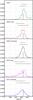 |
Fig. 1 Normalized histogram of the time delays in 1000 realizations of model A, low variability, for various methods: χ2 (upper panel), ZDCF and ICCF methods (lower panels). For ZDCF and ICCF we show results both for the maximum and Gaussian centroid methods of delay determination, for χ2 method we give only the maximum method. The vertical bar marks the assumed lag value. The bottom horizontal bar marks standard deviations of the recovered values from the assumed one. The top horizontal bar marks 0.25−0.75 quantile spread of the recovered histogram. Although the average value describes well the true delay inserted into the model, there is a considerable tail of much shorter or much longer values that contributes considerably to the overall dispersion. |
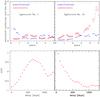 |
Fig. 2 Two examples of the artificial photometric (open red circles) and spectroscopic (filled blue squares) lightcurves and the corresponding plots of the ICCF for model A. Errorbars in the lightcurves (examples shown in the upper-right corners) are not much larger than the points. |
3.1. Dependence on the delay measurement method
3.1.1. ICCF problem
The distribution of the delays obtained for 1000 realizations of the model A, low variability level is shown in Fig. 1. The distribution contains a significant tail of measured time delays that are shorter than the assumed value. The presence of the tail skews the distribution (the mean delay is 549 days, while the median is 605), which enhances the expected error of the time delay measurement. If we simply neglect the solutions with the delay smaller than 500, then the resulting delay is 692 ± 165; if in addition we skip the delays longer than 820 days, the estimated delay is 626 ± 83, i.e., the error is much lower than previously, but we then skip 32.8% of the cases. For the higher variability level the longer delay tail is less important, but the shorter delay tail is very important. If we use the Gaussian centroid instead of the maximum, the histogram of the delays is smoother and the dispersion somewhat lower, but in several cases we do not obtain any solution to the delay measurement.
Thus with ICCF method, the tails of the distribution strongly affect the results. In the real situation we will have just one lightcurve for a single object, so there is a considerable probability that the measurement for a single lightcurve will be completely wrong. We should therefore characterize the probability of the proper delay recovery more accurately. For a simple Gaussian distribution, one parameter describes both the spread of the distribution core and the extent of its tails. The first relates to precision of estimates, the second describes reliability, i.e., probability of a gross error. Delay statistics1 based on our simulations have strongly non-Gaussian distribution, hence at least two parameters are needed to characterize their precision and reliability. For the latter characteristics we selected standard deviation (s.d.) for the former half spread of symmetric quantiles limiting the central 68.3% of the distribution.
To illustrate better the source of such large errors, we plot two examples of the lightcurve realization for model A, and the corresponding ICCF plots (see Fig. 2). The problem is even more severe if the overall variability amplitude is assumed to be lower, although in this case the large outbursts happen less frequently. The ICCF still frequently returns spurious results when the lightcurves are dominated by a single monotonic event (flare) in the observed window. In addition, lower amplitude makes the observational errors relatively more important, so the overall accuracy of the delay determination is lower.
This suggests a considerable space, and actual need, for improvement. Therefore, we consider various alternatives to the ICCF method. To evaluate performance of the delay statistics we employ two criteria: its bias and the error. Inspection of histograms obtained from our simulation reveals asymmetric distribution of the values of the statistics and so we prefer median rather than average value for the estimation of bias. For an arbitrary distribution the former yields equal probability of underestimated and overestimated results. For the estimation of error we employ standard deviation with respect to the assumed delay value of 660 days. As it depends on the quadratic norm of residuals it is sensitive to gross errors. As we aim to minimize the gross errors, the standard deviation seems to be the right choice. However, to better characterize our resulting distribution we also list the half spread of their 1−0.158 and 0.158 quantiles. For the Gaussian distribution it would correspond to half of the ±1σ range, i.e., to 1σ. A small value of the spread compared to the standard deviation indicates a distribution with narrow core and broad wings. We note that generally in case of an asymmetric distribution the position of the center of the spread range does not coincide with the median or average. The corresponding values for all the setups are given in Tables 1 and 2.
3.1.2. χ2 method
In this method we shift the spectroscopic curve and interpolate to the photometric time measurements as we did before, but instead of computing ICCF, we minimize the function 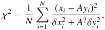 (1)where xi is the photometric flux, yi is the interpolated line flux, δxi is the photometric error, δyi is the spectroscopic error, and N is the number of photometric points. The constant A that adjusts the normalization of the two curves can be obtained analytically from the condition of minimizing the function with respect to A,
 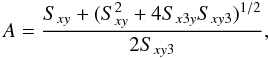 (2)with the coefficients given by
 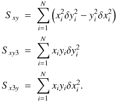 (3)The method works properly only when the searched time delays are smaller than one half of the campaign duration. For longer delays the method picks up the longest values of the time delay since this leaves only relatively short data sequences, where the variability is low because of the red-noise character of the curves, and then the two curves can be fitted very well independently of their actual shape.
3.1.3. ZDCF method
We also analyzed the delay between the simulated photometric and spectroscopic curves using the discrete correlation function (DCF). The idea is rather simple: all possible pairs are formed from two observation sets and then they are binned according to their time lag. The hitch is in the details of statistical evaluation of the bin mean and variance. Here we rely on the Z-transformed discrete correlation function (ZDCF) flavor of the method (Alexander 1997), where the data variance is estimated directly from internal scatter within the bin and not from external error estimates. This method was also used by Kaspi et al. (2007) in their analysis of the HET reverberation results.
The original f77 code by Dr. Alexander was reimplemented in f90 and f2py to form part of the Python time series package (Schwarzenberg-Czerny 2012). Similarly, our Fortran simulation code was called via Python wrapper. In doing so we took care to preserve continuity of our random series between separate Fortran calls.
For each of the 1000 simulations of light curves calculated for a fixed parameter set we analyzed the DCF obtained from the ZDCF algorithm. To decrease scatter of the DCF it was smoothed with the 3-point running median filter. For each smooth DCF we determined its maximum for positive lags λm and attempted to fit it with a Gaussian centroid function f(λ) with four parameters pi,i = 1,··· ,4, i.e., ![Mathematical equation: \hbox{$f(\lambda)=p_0+p_1\exp\left[-\frac{(\lambda-p_4)^2}{2p_3^2}\right].$}](/articles/aa/full_html/2013/08/aa20832-12/aa20832-12-eq117.png) The fit performed with the Python scipy.optimize.curve_fit succeeded on 98% of the occasions. So although the centroid could have been calculated for the majority of the cases, we decided to use the maximum since it always worked and in general did not cause problems.
The fit performed with the Python scipy.optimize.curve_fit succeeded on 98% of the occasions. So although the centroid could have been calculated for the majority of the cases, we decided to use the maximum since it always worked and in general did not cause problems.
Accuracy of the delay recovery for setup A, variability amplitude 0.1, assumed delay 660 days, as a function of the Gaussian width of the BLR response.
The results of simulations yielded histograms of the maximum lag λm and the centroid lag λc ≡ p4 statistics (Fig. 1). From them we conclude that the maximum of DCF statistics λm yields the more precise and robust estimate of the true delay. As far as the limited scope of our simulations permits us to establish, the scatter of the λm statistics around its peak is less than that of λc. Additionally, within the precision of our simulations, we were not able to find any bias of the estimated delay (lag of the histogram peak).
3.2. Dependence on the source variability
For a fixed method, the accuracy of the measurement depends on the adopted level of the variability, as seen from comparison of Tables 1 and 2. Our dimensionless variability amplitude does not translate directly to Fvar since we exponentiated the curves to assure the proper statistical behavior, including the reproduction of the linear dependence of the rms-flux. The actual Fvar of our lightcurves is thus slightly higher, about 15% in a 5 yr timescale for the adopted 0.1 level. Since quasars monitored by HET (Kaspi et al. 2007) showed Fvar within the range from 0.03 to 0.124, we also calculated examples of the setup A for amplitudes of 0.05 and 0.03 using the χ2 method. The recovered delays were 655 ± 204 and 635 ± 232, respectively. If the variability level is indeed that low, the accuracy of the measurement should be higher to assess the requested accuracy of the delay measurement. Even better, more advance methods of the delay measurement, such as those based on damped random walk process (see Zu et al. 2011; Grier et al. 2012a,b) can also help to reduce the expected dispersion in a single measurement.
3.3. Dependence on the BLR transfer function
In the previous section we simply parameterized the reprocessing by the BLR by a shift and convolution with a Gaussian of a fixed width of 10% of the delay. Zu et al. (2011) used a top-hat model of a transfer function. However, the BLR is quite complex and the actual transfer function is more complicated. Previous papers have already pointed towards the considerable difficulties in solving this inversion problem (e.g., Krolik & Done 1995), but already indicated the Keplerian component of the motion with considerable turbulence and net inflow (analysis of the C IV in NGC 5548, Done & Krolik 1996). In recent high-quality data the true BLR complexity shows up pointing towards inflow, outflow, and the presence of the virialized gas in different proportions in different objects (e.g., Denney et al. 2009; Bentz et al. 2008, 2009b; Kollatschny 2003; Grier et al. 2012a,b).
Recent high-quality reverberation results for nearby Seyfert galaxies allowed to reconstruct the transfer function for a spectral range including the Hβ line (Bentz et al. 2010; Grier et al. 2013). For most of the objects at the centroid of Hβ, the transfer fuction is roughly Gaussian, but the width varies from ~20% to 60% (for Mrk 1501). Therefore, for our representative case A, amplitude 0.1, and χ2 method we calculated the time delay accuracy for the increasing width of the Gaussian response. The results are given in Table 3. The accuracy of the delay measurement slowly decreases with the broadening of the BLR transfer function, but the effect is not strong. The red-noise character of the variability leads to non-monotonic dependence even for 1000 statistical realizations. If the lightcurve happens to have a well defined strong minimum or maximum, the measurement is much more accurate than when there is no single strong feature. This is also expected to be the case in real quasar lightcurves.
Other authors, like Bottorff et al. (1997), Pancoast et al. (2011), and Goad et al. (2012) used a physically justified model of the BLR structure which allows a library of velocity-resolved or unresolved transfer functions to be created for comparison with the data. A velocity-unresolved transfer function actually has a Gaussian shape for a face-on disk, but starts at zero lag for a ring (Pancoast et al. 2011). Goad et al. (2012) predict a very shallow transfer function with a peak at intermediate delays for typical parameters.
We incorporated an exemplary transfer function from Goad et al. (2012), their Fig. B.2, inclination 30°, isotropic continuum or disk-like irradiation. The peak of the transfer function in Goad et al. was at 15 days so we simply rescaled the transfer function by a factor of 44 to have the peak at 660 days, as in previous simulations. For isotropic continuum with observational setup A, we recover the delay, although with a considerable error (678 ± 238), and the error is not much smaller for disk-like irradiation (680 ± 230).
The models above are parametric, without the physics underlaying the shape of the bowl. Therefore, considerable theoretical effort in this direction is clearly needed, as the high-quality data for tests start to become available.
4. Discussion
We consider in detail the prospects of determining the dark energy distribution from the reverberation studies of high-redshift quasars, as proposed by Watson et al. (2011). Our motivation comes from the observational campaign with this aim, done with the SALT telescope. However, measuring the delay between UV lines and the continuum in high-redshift quasars is a telescope time consuming project and so a careful analysis performed beforehand can help to optimize it.
Our Monte Carlo simulations of the planned monitoring program of high-redshift AGN show that the success of the monitoring crucially depends on three factors:
-
the choice of the mathematical method to determine the delay;
-
the measurement accuracy;
-
the choice of the emission line.
It is also affected to some extent by other factors like the campaign duration and the distribution of the times of spectroscopic and photometric measurements. These in fact are related to some extent to the choice of the quasars to be monitored. The simulated observational setup mimicked well what we can have for a single quasar with a large telescope, including sparse unevenly distributed spectroscopic observations with gaps for the invisibility of the source.
The choice of the method used to determine the delay does not have to be made in advance, but the estimate of the accuracy achievable in the whole project depends directly on this decision. We have checked three methods: interpolated cross correlation function (ICCF), Z-transformed discreet cross correlation function (ZDCF), and χ2 fitting. The first method almost always gave the largest error. The ZDCF was much better, although occasionally it also failed because of the development of the strong low values tail of the time delay histogram. The results were somewhat better if a Gaussian centroid fit was used instead of a maximum of the histogram, but in a few per cent of the cases the centroid method failed. The χ2 method was usually the most stable one, although it showed a tail at large delays. Therefore, it seems that the best strategy for a real observation is to use both ZDCF and χ2, and compare the results. An even more advanced method based on modeling stochastic processes was introduced by Zu et al. (2011) and its application to a number of sources also shows that it gives much lower errors than CCF (Grier et al. 2012a,b). We did not use this method with our simulated data, but it certainly should be included in the package when analyzing expected observational data.
The accuracy of the photometric and spectroscopic measurements is particularly important if the variability of the quasar is low (observed Fvar less than 0.2 in a five-year campaign). If the campaign lasts much longer and/or variability is much stronger, then the measurement errors are less important, since the red-noise variability in the lightcurves will dominate the measurement scatter.
The choice of the emission line for monitoring is absolutely crucial. Our simulated results given in Tables 1 and 2 were obtained assuming that there is no strong intrinsic variability in the line itself, and the observed variability is due to reprocessing of the variable continuum, broadened with a Gaussian response of the BLR. Indeed, it seems that low ionization lines (LIL) do not show intrinsic variability, and this was the source of the success of the Hβ monitoring. We plan to use another LIL, Mg II 2978 Å, which is also likely just to reflect the nuclear variability. However, if one wants to use the C IV line, which is actually necessary for monitoring quasars at redshifts z > 2, a problem appears: C IV lines belongs to the high ionization line (HIL) class, and so comes from a different part of the BLR. As shown by the results of the HET campaign (Kaspi et al. 2007), in most cases Fvar of the C IV line was much higher than Fvar of the continuum, implying a strong intrinsic variability of the line, and only one tentative measurement was obtained. This is discussed further in the next sections.
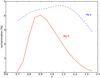 |
Fig. 3 Contamination of the V-band photometry by Mg II 2800 Å and Fe II pseudo-continuum as a function of the quasar redshift. |
On the other hand, monitoring in Mg II also poses additional problems. The continuum variations are followed using broadband V photometry. At some redshift range this leads to contamination of the continuum measurement by the line itself and, more importantly, by the underlying Fe II pseudo-continuum. We modeled the problem representing Mg II as a line of fixed EW of 20 Å and for fixed kinematic width (full width at half maximum, FWHM) of 2500 km s-1. To account for Fe II contamination in the V photometric filter, we used empirical templates of iron emission bands. Vestergaard & Wilkes (2001) constructed their templates by identifying Fe II emission in I Zw 1 AGN in the range 1100−3100 Å with the most significant emission covering the range from 2000 Å to 2900 Å. To extend iron coverage to 3500 Å we incorporated the Tsuzuki et al. (2006) template which is based on emission fitting in nearby quasars. Those two templates show very good agreement in their overlapping range. This allowed us to effectively trace iron contribution to the V band in the redshift range that we were interested in, 0.8−1.4. While the Mg II contamination is clearly unimportant, Fe II contributes up to 5% of the flux to the V band for a source at the redshift of 0.9, but drops down below 3% at z > 1.3 (see Fig. 3).
4.1. Mg II vs. C IV line properties and prospects of monitoring
Mg II line properties correlate well with the properties of the Balmer lines in large quasar samples (Salviander et al. 2007; McGill et al. 2008; Shen et al. 2008; Wang et al. 2009; Shen & Liu 2012). The line was successfully used for black hole mass determination from a single epoch method by a number of authors (McLure & Jarvis 2002; Vestergaard & Osmer 2009; Shen et al. 2011).
Woo (2008) showed that for the Mg II line the variability level is in most cases comparable to the continuum variability. However, one out of five quasars under study (the object CTS300) actually showed much higher variability in Mg II line (rms of 17%) than in 3000 Å continuum (rms of 7%). The reason for this variability is unclear since otherwise this source has similar parameters to the other four objects.
Although some initial studies showed good correlation of the line properties (Vestergaard 2002; Vestergaard & Peterson 2006), more recent results show that C IV line properties correlate poorly with Balmer lines in a given object (Baskin & Laor 2005; Netzer et al. 2007; Shen & Liu 2012). We discuss this issue in detail below.
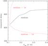 |
Fig. 4 Predicted time delays in 1000 realizations of the model using the of χ2 method, with the observational setup for HET monitoring and assumed 660 day delay inserted in simulations. There is a considerable pile in the last two bins of the delay histogram at the longest time delay that increases with increasing intrinsic variability from 5% to 26%. |
4.2. The problem of C IV monitoring
In the reverberation project for high-redshift quasars with the HET telescope and the C IV line (Kaspi et al. 2007) the obtained results were inconclusive, with only one measurement of a tentative delay of 595 days in S5 0836+71. Here we reproduce the key properties of the monitoring: (i) objects were observable for six months only; typically (not always) three measurements were done, separated by 2.5 months; and (ii) for S5 0836+71 the continuum variability amplitude was Fvar = 0.124, while the mean uncertainty for continuum measurements was 2%, and 10% for the C IV line.
We calculate the predicted delay as a function of the C IV variability level, considering that the line also shows intrinsic variability in addition to the response to variable continuum. We model the intrinsic line variability by formally increasing its measurement error, and we performed computations for this setup using the χ2 method, which usually give the best results. The variability level of the continuum is only slightly lower than in our model A, low variability case (see Table 1), but the spectroscopic and photometric covering is much lower. For Fvar(CIV) = 0.233 the recovered delay is 805 ± 265. One sigma error is large (see Fig. 4), and the upper limit is not well constrained, with 23.7% of the delays stored in the last two histogram bins. The main problem here is not the spectroscopic coverage: without the large intrinsic variability we would recover the delay 650 ± 36 days for the same observational pattern.
This means that C IV monitoring in these sources would require unrealistically long observations for the intrinsic red-noise variability of the continuum to dominate over the intrinsic variations of C IV. Therefore, a better way would be still to use the Mg II line and do the line observations in the near-IR band in the case of sources with considerable intrinsic variability of C IV.
However, in the case of low-redshift Seyfert galaxies NGC 5548 (Clavel et al. 1991), and NGC 3783 (Reichert et al. 1994), the delay of C IV was actually better constrained that the delay of Mg II, and in these two sources the level of variations in C IV was not higher than in the continuum. It might be connected to the recent result of Kruczek et al. (2011) that quasars showing hard X-ray spectra, and thus relatively similar to Seyfert 1 galaxies, do not show strong signatures of outflows, while quasars having soft X-ray spectra, more similar to Narrow Line Seyfert 1 galaxies, do display large C IV shifts. Two classes of quasars, Population A and Population B, were also discussed by Sulentic and collaborators in a number of papers (see, e.g., Sulentic et al. 2007). The behavior is probably controlled by the source Eddington ratio, as argued by Wang et al. (2011) on the basis of their comparative study of C IV and Mg II lines in a sample of AGN selected from SDSS. The sources selected by the HET team generally show rather narrow Mg II lines. Two sources, S4 0636+68 and S5 0836+71, were studied in the IR, and the FWHM of Mg II was determined to be 2850 km s-1 and 3393 km s-1, respectively (Iwamuro et al. 2002). For the remaining four objects studied spectroscopically by Kaspi et al. (2007), we roughly estimated the FWHM (SBS 1116+603 ~ 4000 km s-1, SBS 1233+594 ~ 4500 km s-1, SBS 1425+606 ~ 7520 km s-1, HS 1700+6416 ~ 5300 km s-1) using SDSS data (Adelman-McCarthy et al. 2007), and the object with the very broad line did show the comparable variability in the line and the continuum. In addition, the first three objects are rather radio active, with the flux at 1010 Hz at a similar level to the radio loud composite of Elvis et al. (1994) in comparison with the optical band, and for the remaining three objects there was no radio data in NED. This means that better understanding of the coupling between C IV variability and the remaining properties is clearly needed, and with proper selection the monitoring of distant quasars with C IV can be successful.
4.3. Consequences for cosmology
Our simulations indicate that the reverberation measurements in the Mg II line for quasars at z > 1 can be succesful. This is an interesting project in itself, but the basic goal is to apply these results to cosmology. This requires not only the determination of the time delay between the Mg II line and the continuum for each quasar, but one essential additional step. Having the delay, we determine the absolute quasar monochromatic luminosity of a given quasar, as outlined below. At this point quasars can be used in cosmology in the same way as SN Ia. The essential steps are the following.
For every quasar we plan to determine the observed monochromatic luminosity directly from photometry, the size of the BLR, RBLR, directly from the time delay, and the intrinsic (absolute) monochromatic luminosity in our method is now obtained from the relation ![Mathematical equation: \begin{equation} \log R_{\rm BLR}[{\rm MgII}] = 1.495 + 0.5 \log \, L_{44,2897}, \label{eq:RBLR} \end{equation}](/articles/aa/full_html/2013/08/aa20832-12/aa20832-12-eq149.png) (4)in the quasar rest frame. Here we recalculated the relation from Czerny & Hryniewicz (2011) to the Mg II line wavelength. This relation is based on the assumption of the disk effective temperature Teff = 1000 K at the onset of the BLR, owing to the dust formation in the disk atmosphere. If the dust properties are independent of redshift, there is no error in the constants in this formula.
(4)in the quasar rest frame. Here we recalculated the relation from Czerny & Hryniewicz (2011) to the Mg II line wavelength. This relation is based on the assumption of the disk effective temperature Teff = 1000 K at the onset of the BLR, owing to the dust formation in the disk atmosphere. If the dust properties are independent of redshift, there is no error in the constants in this formula.
The size of the BLR is measured from the line-continuum time delay, and the accuracy is given in Tables 1 and 2. Adopting a realistic setup (model A, χ2 method) we thus gave 5% accuracy in photometry and 17% accuracy in time delay, which translates to the 17% error in the luminosity distance. If we assume that much better accuracy can be actually achieved (model B, χ2 method) the final error reduces to 3%.
It is more convenient to express this using the distance modulus (in magnitudes) defined as  (5)where dL(z) is the luminosity distance in megaparsecs and m and M are, respectively, the apparent and absolute luminosity of the source. The accuracy achievable in our method for a single source translates to 0.34 mag in the first case and 0.06 mag in the second case, for a single object. By monitoring more objects we can increase the accuracy.
Our reverberation project can thus be applied to determine the dark energy distribution much in the same way as SNe Ia. The key question is only whether the accuracy of the measurement of the absolute luminosity, or the distance modulus, is high enough to tell anything about the cosmological models.
To see whether this accuracy is likely to bring interesting results we compare it with several cosmological models. For a given cosmological model one can compute the distance modulus as a function of redshift and compare it with observations. In Fig. 5 we plot residua of distance moduli with respect to the fiducial ΛCDM model, μmod − μfid, assuming null spatial curvature (generalization to non-flat models is straightforward). We show two wCDM models with a constant equation of state of dark energy w = −0.8 and w = −1.2, and one with variable w(z) = w0 + waz/(1 + z) (the w0waCDM model). The fiducial cosmological parameters used were the central values obtained by Mehta et al. (2012): Ωm = 0.28 and H0 = 70 km s-1 pc-1 in case of the ΛCDM and wCDM models, and Ωm = 0.272, H0 = 71 km s-1 Mpc-1, w0 = −1.02, and wa = −0.26 for the w0waCDM model.
Since the expected differences between different cosmological models are on the order of 0.1 mag, it is possible to test the cosmological models with quasars at z ~ 1, if the measurement accuracy and/or the number of sources is high.
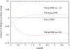 |
Fig. 5 Residua of distance moduli μmod − μfid (in magnitudes) with respect to the fiducial ΛCDM model for two wCDM models with constant equation of state and one w0waCDM model with variable w(z). |
4.4. Limitations of the method, sources of systematic errors, and future method developments
Quasars are now being observed up to redshifts above 7 (ULAS J1120+0641, z = 7.085, Mortlock et al. 2011). The monitoring in the optical band based on Mg II line is applicable only to 0.5 < z < 1.5 quasars. For higher redshifts, lines like C IV and Lyα must then be used to trace BLR. Our current method using Mg II is based on applicability of Eq. (4), i.e., on the assumption that lines form close to the atmosphere of a Keplerian disk, and the line emitting clouds should not show systematic departure from the Keplerian motion as well, apart from a turbulent motion up and down due to subsequent condensation and evaporation of the dust (Czerny & Hryniewicz 2011). Low-ionization lines like Hβ and Mg II satisfy this condition approximately, although some evidence for inflow is seen even in the Balmer lines (Grier et al. 2013). In the case of C IV the evidence of outflow is well established, and it is strong in some quasars but moderate in others (see Kruczek et al. 2011 for recent determinations of C IV blueshift and its relation with the overall quasar spectrum). This motion has to be taken into account when relating the black hole mass, monochromatic luminosity and the position of the specific line, so Eq. (4) has to be replaced by a more complex theory of the BLR formation. In the case of a specific object, the viewing angle is also an issue although in a statistical approach using many objects, this may average to some extent. Systematic errors of the method are now difficult to specify, but future studies of the transfer function in the nearby sources and corresponding development of the BLR modeling are absolutely necessary.
The second assumption underlying Eq. (4) is the assumption that the dust properties are universal in all quasars. Dust provides the driving force behind the rise and fall of the clouds and explains the large covering factor of the BLR; if dust composition is a function of redshift, the dust evaporation temperature would also depend on the quasar redshift. Specifically, since graphite grains have a higher evaporation temperature and silicates and amorphous grains have a lower evaporation temperature, the mean effect depends on the chemical composition of the disk atmosphere. Fortunately, the knowledge of nearby sources can probably apply to high-redshift quasars because of the small metallicity gradient with redshift in quasar populations, and because all high Eddington luminosity sources have somewhat super-solar metallicity, both locally and for high-redshift sources (e.g., Simon & Hamann 2010).
4.5. Comparison of the quasar method with other methods
The current dark energy constraints already come from various research lines. All methods can be divided into standard ruler methods and standard candle methods. Standard ruler methods rely on the determination of a true or characteristic size and on measurements of the apparent size, and most current methods belong to this class (microwave background modeling, all large-scale structure methods including BAO, power spectra and void studies, weak lensing, galaxy cluster methods). Our method, based on the determination of the quasar intrinsic luminosity, clearly belongs to the second family, the standard candle methods, together with the supernovae Ia and gamma-ray burst methods. If considered in the ΩΛ vs. Ωm space, these methods usually give considerably elongated contour errors, roughly perpendicular to each other. This is the reason why a combination of the two methods is usually used to give strong constraints on the cosmological models. Our method has the same in-built degeneracy as the supernovae Ia, and it would also need to be combined with complementary constraints (e.g., new results from Planck mission) to break it.
The advantage of the method is that it can easily cover a somewhat higher redshift range than supernovae (the groud-based observations of SNe Ia do not extend beyond z = 1, Regnault et al. 2009; the HST observations are needed to bring objects 0.623 < z < 1.415, Suzuki et al. 2012). Methods based on gamma-ray bursts can go much farther, but they still need much more study to achieve the proper understanding. Quasars are bright and numerous. On the other hand, the reverberation studies are time consuming, and the delays increase with redshift unless we go to fainter objects containing fewer massive black holes than the extreme bright sources. Thus, single-object observations like long-slit spectroscopy with SALT cannot bring many measurements. However, multi-object spectroscopic studies can bring the data suitable for application of our method. Current instruments like LAMOST may in principle perform such studies (see, e.g., Wu et al. 2010) if working at full capacity. Among the planned missions EUCLID, with its six-year lifetime, would also be perfect for that purpose, although the mission is aimed at covering large area of the sky without many repeated observations of the same area.
Here statistics means a function of data used for estimates.
Acknowledgments
Part of this work was supported by the Polish grant No. 719/N-SALT/2010/0, and by the grants 2011/03/B/ST9/03281 and DEC-2011/03/B/ST9/03459 from the National Science Center. B.C. and K.H. acknowledge the support from the Foundation for Polish Science through Master/Mistrz program. The financial assistance of the South African National Research Foundation (NRF) towards this research is hereby acknowledged (MB). A.S.C. was funded by grant NCN 2011/01/M/ST9/05914. This publication makes use of data products from the Sloan Digital Sky Survey. Funding for the SDSS and SDSS-II has been provided by the Alfred P. Sloan Foundation, the Participating Institutions, the National Science Foundation, the US. Department of Energy, the National Aeronautics and Space Administration, the Japanese Monbukagakusho, the Max Planck Society, and the Higher Education Funding Council for England. The SDSS Web Site is http://www.sdss.org/. This research has also made use of the NASA/IPAC Extragalactic Database (NED) which is operated by the Jet Propulsion Laboratory, California Institute of Technology, under contract with the National Aeronautics and Space Administration.
References
- Adelman-McCarthy, J. K., Agüeros, M. A., Allam, S. S., et al. 2007, ApJS, 172, 634 [NASA ADS] [CrossRef] [Google Scholar]
- Alexander, T. 1997, in Is AGN Variability Correlated with Other AGN Properties? ZDCF Analysis of Small Samples of Sparse Light Curves in Astronomical Time Series, eds. D. Maoz, A. Sternberg, & E. M. Leibowitz, Astrophys. Space Sci. Lib., 218, 163 [Google Scholar]
- Amendola, L., & Tsuikawa, S. 2010, Dark energy (Cambridge University Press) [Google Scholar]
- Barbieri, C., Cappellaro, E., Turatto, M., Romano, G., & Szuszkiewicz, E. 1988, A&AS, 76, 477 [NASA ADS] [Google Scholar]
- Barth, A. J., Nguyen, M. L., Malkan, M. A., et al. 2011, ApJ, 732, 121 [NASA ADS] [CrossRef] [Google Scholar]
- Baskin, A., & Laor, A. 2005, MNRAS, 356, 1029 [NASA ADS] [CrossRef] [Google Scholar]
- Bauer, A., Baltay, C., Coppi, P., et al. 2009, ApJ, 696, 1241 [NASA ADS] [CrossRef] [Google Scholar]
- Benson, B. A., de Haan, T., Dudley, J. P., et al. 2013, ApJ, 763, 147 [NASA ADS] [CrossRef] [Google Scholar]
- Bentz, M. C., Walsh, J. L., Barth, A. J., et al. 2008, ApJ, 689, L21 [NASA ADS] [CrossRef] [Google Scholar]
- Bentz, M., Peterson, B. M., Netzer, H., et al. 2009a, ApJ, 697, 160 [Google Scholar]
- Bentz, M., Walsh, J. L., Barth, A. J., et al. 2009b, ApJ, 705, 199 [NASA ADS] [CrossRef] [Google Scholar]
- Bentz, M., Horne, K., Barth, A. J., et al. 2010, ApJ, 720, L46 [NASA ADS] [CrossRef] [Google Scholar]
- Bian, W., & Yang, Z. 2011, JA&A, 32, 253 [NASA ADS] [Google Scholar]
- Biesiada, M., & Piorkowska, A. 2009, MNRAS, 396, 946 [NASA ADS] [CrossRef] [Google Scholar]
- Blandford, R. D., & McKee, C. F. 1982, ApJ, 255, 419 [NASA ADS] [CrossRef] [EDP Sciences] [Google Scholar]
- Bottorff, M. C., Korista, K. T., Shlosman, I., & Blandford, R. D. 1997, ApJ, 479, 200 [NASA ADS] [CrossRef] [Google Scholar]
- Chelouche, D., Daniel, E., & Kaspi, S. 2012, ApJ, 750, L43 [NASA ADS] [CrossRef] [Google Scholar]
- Chevallier, M., & Polarski, D. 2001, IJMPD, 10, 213 [Google Scholar]
- Clavel, J., Reichert, G. A., Alloin, D., et al. 1991, ApJ, 366, 64 [NASA ADS] [CrossRef] [Google Scholar]
- Cristiani, S., Trentini, S., La Franca, F., et al. 1996, A&A, 306, 395 [NASA ADS] [Google Scholar]
- Czerny, B., & Hryniewicz, K. 2011, A&A, 525, L8 [NASA ADS] [CrossRef] [EDP Sciences] [Google Scholar]
- Czerny, B., Schwarzenberg-Czerny, A., & Loska, Z. 1999, MNRAS, 303, 148 [NASA ADS] [CrossRef] [Google Scholar]
- Czerny, B., Nikolajuk, M., Piasecki, M., & Kuraszkiewicz, J. 2001, MNRAS, 325, 865 [NASA ADS] [CrossRef] [Google Scholar]
- Czerny, B., Doroshenko, V. T., Nikołajuk, M., et al. 2003, MNRAS, 342, 1222 [NASA ADS] [CrossRef] [Google Scholar]
- Dainotti, M. G., Ostrowski, M., & Willingale, R., 2011, MNRAS, 418, 2202 [NASA ADS] [CrossRef] [Google Scholar]
- Denney, K. D., Watson, L. C., Peterson, B. M., et al. 2009, ApJ, 702, 1353 [NASA ADS] [CrossRef] [Google Scholar]
- Denney, K. D., Peterson, B. M., Pogge, R. W., et al. 2010, ApJ, 721, 715 [NASA ADS] [CrossRef] [Google Scholar]
- De Rosa, G., Decarli, R., Walter, F., et al., 2011, ApJ, 739, 56 [NASA ADS] [CrossRef] [Google Scholar]
- Dietrich, M., Hamann, F., Appenzeller, I., & Vestergaard, M. 2003a, ApJ, 596, 817 [NASA ADS] [CrossRef] [Google Scholar]
- Dietrich, M., Hamann, F., Shields, J. C., et al. 2003b, ApJ, 589, 722 [NASA ADS] [CrossRef] [Google Scholar]
- Dietrich, M., Peterson, B. M., Grier, C. J., et al. 2012, ApJ, 757, 53 [NASA ADS] [CrossRef] [Google Scholar]
- Done, C., & Krolik, J. H. 1996, ApJ, 463, 144 [NASA ADS] [CrossRef] [Google Scholar]
- Edelson, R. A., Alexander, T., Crenshaw, D. M., et al. 1996, ApJ, 470, 364 [NASA ADS] [CrossRef] [Google Scholar]
- Eisenstein, D. J., Zehavi, I., Hogg, D. W., et al. 2005, ApJ, 633, 560 [NASA ADS] [CrossRef] [Google Scholar]
- Elvis, M., Wilkes, B. J., McDowell, J. C., et al. 1994, ApJS, 95, 1 [NASA ADS] [CrossRef] [Google Scholar]
- Frieman, J. A., Turner, M. S., & Huterer, D. 2008, ARA&A, 46, 385 [NASA ADS] [CrossRef] [Google Scholar]
- Gall, C., Andersen, A. C., & Hjorth, J. 2011, A&A, 528, A14 [NASA ADS] [CrossRef] [EDP Sciences] [Google Scholar]
- Gaskell, C. M., & Peterson, B. M. 1987, ApJS, 65, 1 [NASA ADS] [CrossRef] [Google Scholar]
- Goad, M. R., Korista, K. T., & Ruff, A. J. 2012, MNRAS, 426, 3086 [NASA ADS] [CrossRef] [Google Scholar]
- Grier, C., Peterson, B. M., Pogge, R. W., et al. 2012a, ApJ, 744, L4 [NASA ADS] [CrossRef] [Google Scholar]
- Grier, C., Peterson, B. M., Pogge, R. W., et al. 2012b, ApJ, 755, 60 [NASA ADS] [CrossRef] [Google Scholar]
- Grier, C., Peterson, B. M., Horne, K., et al. 2013, ApJ, 764, 47 [NASA ADS] [CrossRef] [Google Scholar]
- Guzzo, L., Pierleoni, M., Meneux, B., et al. 2008, Nature, 451, 541 [NASA ADS] [CrossRef] [PubMed] [Google Scholar]
- Hawkins, M. R. S. 1983, MNRAS, 202, 571 [NASA ADS] [Google Scholar]
- Hayashida, K., Miyamoto, S., Kitamoto, S., Negoro, H., & Inoue, H. 1998, ApJ, 500, 642 [NASA ADS] [CrossRef] [Google Scholar]
- Hewett, P. C., Foltz, C. B., & Chaffee, F. H. 1995, AJ, 109, 1498 [NASA ADS] [CrossRef] [Google Scholar]
- Hinshaw, G., Larson, D., Komatsu, E., et al. 2012, ApJS, accepted [arXiv:1212.5226] [Google Scholar]
- Iwamuro, F., Motohara, K., Maihara, T., et al. 2002, ApJ, 565, 63 [NASA ADS] [CrossRef] [Google Scholar]
- Jain, B., & Taylor, A. 2003, Phys. Rev. Lett., 91, 141302 [NASA ADS] [CrossRef] [PubMed] [Google Scholar]
- Kaspi, S., Smith, P. S., Netzer, H., et al. 2000, ApJ, 533, 631 [NASA ADS] [CrossRef] [Google Scholar]
- Kaspi, S., Brandt, W. N., Maoz, D., et al. 2007, ApJ, 659, 997 [NASA ADS] [CrossRef] [Google Scholar]
- Kofman, L. A., Gnedin, N. Y., & Bahcall, N. A. 1993, ApJ, 413, 1 [NASA ADS] [CrossRef] [Google Scholar]
- Kollatschny, W. 2003, A&A, 407, 461 [NASA ADS] [CrossRef] [EDP Sciences] [Google Scholar]
- Kong, M.-Z., Wu, X.-B., Wang, R., & Han, J.-L. 2006, Chin. J. Astron. Astrophys., 6, 396 [NASA ADS] [CrossRef] [Google Scholar]
- Krolik, J. H., & Done, C. 1995, ApJ, 440, 166 [NASA ADS] [CrossRef] [Google Scholar]
- Kruczek, N. E., Richards, G. T., Gallagher, S. C., et al. 2011, AJ, 142, 130 [NASA ADS] [CrossRef] [Google Scholar]
- Li, M., Li, X.-D., Wang, S., & Wang, Y. 2011, Comm. Theoret. Phys., 56, 525 [Google Scholar]
- MacLoad, C. L., Ivezić, Ž., Sesar, B., et al. 2012, ApJ, 753, 106 [NASA ADS] [CrossRef] [Google Scholar]
- Mattarese, S., Colpi, M., Gorini, V., & Moschella, U. 2011, Dark Matter and Dark Energy, Astrophys. Space Sci. Lib. (Netherlands: Springer) [Google Scholar]
- Matthews, T. A., & Sandage, A. R. 1963, ApJ, 138, 30 [NASA ADS] [CrossRef] [Google Scholar]
- McGill, K. L., Woo, J., Treu, T., & Malkan, M. A. 2008, ApJ, 673, 703 [NASA ADS] [CrossRef] [Google Scholar]
- McHardy, I. M., Koerding, E., Knigge, C., Uttley, P., & Fender, R. P. 2006, Nature, 444, 730 [NASA ADS] [CrossRef] [PubMed] [Google Scholar]
- McLure, R. J., & Jarvis, M. J. 2002, MNRAS, 337, 109 [NASA ADS] [CrossRef] [Google Scholar]
- Mehta, K. T., Cuesta, A. J., Xu, X., Eisenstein, D. J., & Padmanabhan, N. 2012, MNRAS, 427, 2168 [NASA ADS] [CrossRef] [Google Scholar]
- Metzroth, K. G., Onken, C. A., & Peterson, B. M. 2006, ApJ, 647, 901 [NASA ADS] [CrossRef] [Google Scholar]
- Mortlock, D. J., Warren, S. J., Venemans, B. P., et al. 2011, Nature, 474, 616 [NASA ADS] [CrossRef] [PubMed] [Google Scholar]
- Mushotzky, R. F., Edelson, R., Baumgartner, W., & Gandhi, P. 2011, ApJ, 743, L12 [NASA ADS] [CrossRef] [Google Scholar]
- Netzer, H., Lira, P., Trakhtenbrot, B., Shemmer, O., & Cury, I. 2007, ApJ, 671, 1256 [NASA ADS] [CrossRef] [Google Scholar]
- Nikolajuk, M., Czerny, B., & Gurynowicz, P. 2009, MNRAS, 394, 2141 [NASA ADS] [CrossRef] [Google Scholar]
- O’Brien, P. T., Dietrich, M., Leighly, K., et al. 1998, ApJ, 509, 163 [NASA ADS] [CrossRef] [Google Scholar]
- Pancoast, A., Brewer, B. J., & Treu, T. 2011, ApJ, 730, 139 [NASA ADS] [CrossRef] [Google Scholar]
- Papadakis, I. E. 2004, A&A, 425, 1133 [NASA ADS] [CrossRef] [EDP Sciences] [Google Scholar]
- Peebles, P. J. E. 1984, ApJ, 284, 439 [NASA ADS] [CrossRef] [Google Scholar]
- Perlmutter, S., Aldering, G., della Valle, M., et al. 1998, Nature, 391, 51 [CrossRef] [Google Scholar]
- Peterson, B. M. 1993, PASP, 105, 247 [NASA ADS] [CrossRef] [Google Scholar]
- Peterson, B. M., & Wandel, A. 1999, ApJ, 521, L95 [NASA ADS] [CrossRef] [Google Scholar]
- Peterson, B. M., Berlind, P., Bertram, R., et al. 2002, ApJ, 581, 197 [NASA ADS] [CrossRef] [Google Scholar]
- Peterson, B. M., Ferrarese, L., Gilbert, K. M., et al. 2004, ApJ, 613, 682 [NASA ADS] [CrossRef] [Google Scholar]
- Planck Collaboration 2013, A&A, submitted [arXiv:1303.5076] [Google Scholar]
- Ponti, G., Papadakis, I., Bianchi, S., et al. 2012, A&A, 542, A83 [NASA ADS] [CrossRef] [EDP Sciences] [Google Scholar]
- Regnault, N., Conley, A., Guy, J., et al. 2009, A&A, 506, 999 [NASA ADS] [CrossRef] [EDP Sciences] [Google Scholar]
- Reichert, G. A., Rodriguez-Pascual, P. M., Alloin, D., et al. 1994, ApJ, 425, 582 [NASA ADS] [CrossRef] [Google Scholar]
- Riess, A. G., Filippenko, A. V., Challis, P., et al. 1998, AJ, 116, 1009 [NASA ADS] [CrossRef] [Google Scholar]
- Salviander, S., Shields, G. A., Gebhardt, K., & Bonning, E. W. 2007, ApJ, 662, 131 [NASA ADS] [CrossRef] [Google Scholar]
- Sanchez, A. G., Scóccola, C. G., Ross, A. J., et al. 2012, MNRAS, 425, 415 [NASA ADS] [CrossRef] [Google Scholar]
- Schutz, B. F. 1986, Nature, 323, 310 [NASA ADS] [CrossRef] [Google Scholar]
- Schwarzenberg-Czerny, A. 2012, in IAU Symp., 285, 81 [Google Scholar]
- Sergeev, S. G., Malkov, Yu. F., Chuvaev, K. K., & Pronik, V. I. 1994, ASPC, 69, 199 [NASA ADS] [Google Scholar]
- Seto, N., Kawamura, S., & Nakamura, T. 2001, Phys. Rev. Lett., 87, 221103 [NASA ADS] [CrossRef] [PubMed] [Google Scholar]
- Shen, Y., & Liu, X. 2012, ApJ, 753, 125 [NASA ADS] [CrossRef] [Google Scholar]
- Shen, Y., Greene, J. E., Strauss, M. A., Richards, G. T., & Schneider, D. P. 2008, ApJ, 680, 169 [NASA ADS] [CrossRef] [Google Scholar]
- Shen, Y., Richards, G. T., Strauss, M. A., et al. 2011, ApJS, 194, 45 [NASA ADS] [CrossRef] [Google Scholar]
- Simon, L. E., & Hamann, F. 2010, MNRAS, 407, 1826 [NASA ADS] [CrossRef] [Google Scholar]
- Stalin, C. S., Jeyakumar, S., Coziol, R., Pawase, R. S., & Thakur, S. S. 2011, MNRAS, 416, 225 [NASA ADS] [Google Scholar]
- Sulentic, J., Bachev, R., Marziani, P., et al. 2007, ApJ, 666, 757 [NASA ADS] [CrossRef] [Google Scholar]
- Suzuki, N., Rubin, D., Lidman, C., et al. 2012, ApJ, 746, 85 [NASA ADS] [CrossRef] [Google Scholar]
- Terebizh, V. Y., Terebizh, A. V., & Biryukov, V. V. 1989, Ap, 31, 460 [NASA ADS] [Google Scholar]
- Timmer, J., & Konig, M. 1995, A&A, 300, 707 [NASA ADS] [Google Scholar]
- Tsuzuki, Y., Kawara, K., Yoshii, Y., et al. 2006, ApJ, 650, 57 [NASA ADS] [CrossRef] [Google Scholar]
- Ulrich, M.-H., Maraschi, L., & Urry, C. M. 1997, ARA&A, 35, 445 [NASA ADS] [CrossRef] [Google Scholar]
- Uttley, P., McHardy, I. M., & Vaughan, S. 2005, MNRAS, 359, 345 [NASA ADS] [CrossRef] [Google Scholar]
- Van den Berk, D. E., Wilhite, B. C., Kron, R. G., et al. 2004, ApJ, 601, 692 [NASA ADS] [CrossRef] [Google Scholar]
- Vestergaard, M. 2002, ApJ, 571, 733 [NASA ADS] [CrossRef] [Google Scholar]
- Vestergaard, M., & Osmer, P. S. 2009, ApJ, 699, 800 [Google Scholar]
- Vestergaard, M., & Peterson, B. M. 2006, ApJ, 641, 689 [NASA ADS] [CrossRef] [Google Scholar]
- Vestergaard, M., & Wilkes, B. J. 2001, ApJS, 134, 1 [NASA ADS] [CrossRef] [Google Scholar]
- Walsh, J. L., Minezaki, T., Bentz, M. C., et al. 2009, ApJS, 185, 156 [NASA ADS] [CrossRef] [Google Scholar]
- Wandel, A., Peterson, B. M., & Malkan, M. A. 1999, ApJ, 526, 579 [NASA ADS] [CrossRef] [Google Scholar]
- Wang, T.-G., Wamsteker, W., & Cheng, F.-Z. 1997, in ASP Conf. Ser., 113, 155 [Google Scholar]
- Wang, J. G., Dong, X.-B., Wang, T.-G., et al. 2009, ApJ, 707, 1334 [NASA ADS] [CrossRef] [Google Scholar]
- Wang, H., Wang, T., Zhou, H., et al. 2011, ApJ, 738, 85 [NASA ADS] [CrossRef] [Google Scholar]
- Watson, D., Denney, K. D., Vestergaard, M., & Davis, T. M. 2011, ApJ, 740, L49 [NASA ADS] [CrossRef] [Google Scholar]
- Woo, J.-H. 2008, AJ, 135, 1849 [NASA ADS] [CrossRef] [Google Scholar]
- Wu, Xue-Bing, Jia, Z.-D., Chen, Z.-Y., et al. 2010, RAA, 10, 745 [NASA ADS] [Google Scholar]
- Zhou, X.-L., Zhang, S.-N., Wang, D.-X., & Zhu, L. 2010, ApJ, 710, 16 [NASA ADS] [CrossRef] [Google Scholar]
- Zu, Y., Kochanek, C. S., & Peterson, B. M. 2011, ApJ, 735, 80 [NASA ADS] [CrossRef] [Google Scholar]
All Tables
Parameters of the models and the accuracy of the delay recovery for variability amplitude 0.1, assumed delay 660 days.
Parameters of the models and the accuracy of the delay recovery for variability amplitude 0.3, assumed delay 660 days.
Accuracy of the delay recovery for setup A, variability amplitude 0.1, assumed delay 660 days, as a function of the Gaussian width of the BLR response.
All Figures
|
Fig. 1 Normalized histogram of the time delays in 1000 realizations of model A, low variability, for various methods: χ2 (upper panel), ZDCF and ICCF methods (lower panels). For ZDCF and ICCF we show results both for the maximum and Gaussian centroid methods of delay determination, for χ2 method we give only the maximum method. The vertical bar marks the assumed lag value. The bottom horizontal bar marks standard deviations of the recovered values from the assumed one. The top horizontal bar marks 0.25−0.75 quantile spread of the recovered histogram. Although the average value describes well the true delay inserted into the model, there is a considerable tail of much shorter or much longer values that contributes considerably to the overall dispersion. |
| In the text | |
|
Fig. 2 Two examples of the artificial photometric (open red circles) and spectroscopic (filled blue squares) lightcurves and the corresponding plots of the ICCF for model A. Errorbars in the lightcurves (examples shown in the upper-right corners) are not much larger than the points. |
| In the text | |
|
Fig. 3 Contamination of the V-band photometry by Mg II 2800 Å and Fe II pseudo-continuum as a function of the quasar redshift. |
| In the text | |
|
Fig. 4 Predicted time delays in 1000 realizations of the model using the of χ2 method, with the observational setup for HET monitoring and assumed 660 day delay inserted in simulations. There is a considerable pile in the last two bins of the delay histogram at the longest time delay that increases with increasing intrinsic variability from 5% to 26%. |
| In the text | |
|
Fig. 5 Residua of distance moduli μmod − μfid (in magnitudes) with respect to the fiducial ΛCDM model for two wCDM models with constant equation of state and one w0waCDM model with variable w(z). |
| In the text | |
Current usage metrics show cumulative count of Article Views (full-text article views including HTML views, PDF and ePub downloads, according to the available data) and Abstracts Views on Vision4Press platform.
Data correspond to usage on the plateform after 2015. The current usage metrics is available 48-96 hours after online publication and is updated daily on week days.
Initial download of the metrics may take a while.