| Issue |
A&A
Volume 555, July 2013
|
|
|---|---|---|
| Article Number | L8 | |
| Number of page(s) | 5 | |
| Section | Letters | |
| DOI | https://doi.org/10.1051/0004-6361/201321776 | |
| Published online | 11 July 2013 | |
Molecular gas mass functions of normal star-forming galaxies since z ~ 3⋆
1
Max-Planck-Institut für extraterrestrische Physik (MPE),
Postfach 1312,
85741
Garching,
Germany
e-mail: berta@mpe.mpg.de
2
School of Physics and Astronomy, The Raymond and Beverly Sackler
Faculty of Exact Sciences, Tel-Aviv University, 69978
Tel-Aviv,
Israel
3
Argelander-Institut für Astronomie, Universität
Bonn, Auf dem Hügel
71, 53121
Bonn,
Germany
Received: 26 April 2013
Accepted: 7 June 2013
We used deep far-infrared data from the PEP/GOODS-Herschel surveys and restframe ultraviolet photometry to study the evolution of the molecular gas mass function of normal star-forming galaxies. Computing the molecular gas mass, Mmol, by scaling star formation rates through depletion timescales, or combining infrared (IR) luminosity and obscuration properties as described in the literature, we obtained Mmol for roughly 700, z = 0.2−3.0 galaxies near the star-forming main sequence. The number density of galaxies follows a Schechter function of Mmol. The characteristic mass M ∗ is found to strongly evolve up to z ~ 1 and then flatten at earlier epochs, resembling the IR luminosity evolution of similar objects. At z ~ 1, our result is supported by an estimate based on the stellar mass function of star-forming galaxies and gas fraction scalings from the PHIBSS survey. We compared our measurements with results from current models, finding better agreement with those that are treating star formation laws directly rather than in post-processing. Integrating the mass function, we studied the evolution of the Mmol density and its density parameter Ωmol.
Key words: galaxies: luminosity function, mass function / galaxies: statistics / galaxies: evolution / galaxies: star formation / infrared: galaxies
© ESO, 2013
1. Introduction
Stars form in cold, dense molecular clouds, and the molecular gas content of galaxies is an important constraint to galaxy evolution. In the interplay between accretion of gas, star formation, metal enrichment, and outflows, the molecular gas content reflects the prevailing physical processes (e.g. Bouché et al. 2010; Davé et al. 2010; Lilly et al. 2013). For the cosmic baryon budget (e.g. Fukugita et al. 1998), molecular gas can be of increasing relative importance at high redshifts where galaxies are gas-rich.
Molecular gas is generally quantified using the CO molecule as a tracer. Local samples include several hundred targets (e.g. Saintonge et al. 2011, and references therein), but CO detections of star-forming, intermediate- or high-redshift galaxies are still limited to modest statistics of mostly very luminous galaxies (Carilli & Walter 2013, and references therein). For normal star-forming galaxies, the PHIBSS survey (Tacconi et al. 2013) derives scaling relations on the basis of CO detections of 52 normal star-forming galaxies at z ~ 1.2 and z ~ 2.2. In galaxies near the star-forming main sequence (MS, e.g. Noeske et al. 2007; Elbaz et al. 2007; Daddi et al. 2007), the molecular gas mass, Mmol, scales as star formation rate (SFR) through a depletion timescale τdep that only very weakly depends on redshift (Tacconi et al. 2013).
Keres et al. (2003) reported the first attempt of deriving the local molecular gas mass function, based on a sample of IRAS-selected objects. To date, no derivation of a z > 0 mass function has been possible due to the heterogeneity and paucity of the available detections.
These difficulties have sparked interest in methods that use dust mass as a tool for deriving masses of the cold ISM of (distant) galaxies (e.g. Magdis et al. 2011, 2012; Scoville 2012). Dust mass is converted into gas mass by adopting a metallicity and scaling the gas-to-dust ratio with metallicity. In order to derive accurate dust masses, these methods require photometry on the restframe-submm tail of the spectral energy distributions (SED) or accurate multi-band data close to the restframe far-infrared (FIR) SED peak. These requirements are still not met individually for large samples of normal high-z galaxies (Berta et al., in prep.). In a study of the restframe ultraviolet (UV) and FIR properties of Herschel galaxies, Nordon et al. (2013) established a method for deriving Mmol of MS galaxies on the basis of their rest-FIR luminosity and rest-UV obscuration: these properties are readily available for larger samples. Here we apply the τdep scaling and the Nordon et al. recipe to the deepest Herschel (Pilbratt et al. 2010) FIR extragalactic observations and related restframe UV data to derive Mmol of MS galaxies, which are known to power ~90% of the cosmic star formation (Rodighiero et al. 2011). On this basis, we construct their molecular gas mass function and study its evolution since z ~ 3.
We adopt a ΛCDM cosmology with (h,Ωm,ΩΛ) = (0.70, 0.27, 0.73) and a Chabrier (2003) initial mass function.
2. Derivation of molecular gas mass and source selection
We used the deepest PACS (Poglitsch et al. 2010) FIR survey, combining the PACS Evolutionary Probe (PEP, Lutz et al. 2011) and GOODS-Herschel (Elbaz et al. 2011) data in the GOODS-N and GOODS-S fields. We defer to Magnelli et al. (2013) for details about data reduction and catalog extraction.
Ancillary data come from the catalogs built by Berta et al. (2011) and Grazian et al. (2006, MUSIC), both including photometry from the U to Spitzer IRAC bands. To these we added Spitzer MIPS 24 μm (Magnelli et al. 2011), IRS 16 μm data (Teplitz et al. 2011), GALEX DR6 data, and a collection of optical spectroscopic redshifts (see Berta et al. 2011, for details). When needed, photometric redshifts were used, reaching accuracies of Δ(z)/(1 + z) = 0.04 and 0.06 in the two fields, respectively (Berta et al. 2011; Santini et al. 2009).
Based on current CO observations of local and z ~ 1 objects (e.g. Saintonge et al. 2011, 2012; Tacconi et al. 2013), the relation between Mmol and SFR of MS galaxies can be described as a simple scaling with a depletion timescale mildly dependent on redshift: Mmol/SFR = τdep, with τdep = 1.5 × 109 × (1 + z)-1 [Gyr] . Second-order effects, most likely driven by the actual distribution of dust and gas in galaxies, have been studied by Nordon et al. (2013) while investigating the infrared excess (IRX) and the observed UV slope β of 1.0 < z < 2.5 PEP galaxies (Meurer et al. 1999). Using a smaller sample of z ≥ 1 galaxies with CO gas masses, Nordon et al. studied the link between AIRX and molecular gas content, finding a tight relation between the scatter in the AIRX-β plane and the specific attenuation contributed by the molecular gas mass per young star. Here1AIRX = 2.5log (SFRIR/SFRUV + 1) represents the effective UV attenuation. These authors derived the equation ![\begin{equation} \label{eq:SA_method} \log\left(\!\frac{M_{\rm mol}}{[10^9~{M}_\odot]}\!\right)\!=\! \log \left(\! \frac{A_{\rm IRX} \textit{SFR}}{[{M}_\odot\,\textrm{yr}^{-1}]}\!\right)-0.20\left(A_{\rm IRX}\!-\!1.26\beta\right)+0.09\textrm{,} \end{equation}](/articles/aa/full_html/2013/07/aa21776-13/aa21776-13-eq28.png) (1)where the SFR includes both IR and UV contributions. This provides an estimate of molecular gas mass (already including the contribution of helium) using only widely available integrated restframe UV and FIR photometry, consistent with z ~ 1 depletion times by calibration. We used the FIR and UV photometry to apply the Tacconi et al. (2013)τdep scaling and the Nordon et al. (2013) recipe to ~700 MS galaxies in our survey. We stress again that both methods rely on calibrations based on CO observations and are thus valid under the assumption that the adopted values of the CO-to-molecular gas mass conversion factor, αCO, are correct (see Tacconi et al. 2013; Nordon et al. 2013).
(1)where the SFR includes both IR and UV contributions. This provides an estimate of molecular gas mass (already including the contribution of helium) using only widely available integrated restframe UV and FIR photometry, consistent with z ~ 1 depletion times by calibration. We used the FIR and UV photometry to apply the Tacconi et al. (2013)τdep scaling and the Nordon et al. (2013) recipe to ~700 MS galaxies in our survey. We stress again that both methods rely on calibrations based on CO observations and are thus valid under the assumption that the adopted values of the CO-to-molecular gas mass conversion factor, αCO, are correct (see Tacconi et al. 2013; Nordon et al. 2013).
The SFRIR,UV were computed using the Kennicutt (1998) calibrations. Infrared luminosities, L(IR), were derived by SED fitting with the Berta et al. (2013) templates library. Alternative methods (e.g. Wuyts et al. 2011; Nordon et al. 2012) lead to equivalent results within a 10–20% scatter (see Berta et al. 2013). UV parameters were derived from the restframe 1600 and 2800 Å luminosities, following the procedure of Nordon et al. (2013).
Uncertainties on Mmol were computed by combining the systematic errors embedded in the adopted equations and statistical uncertainties due to the scatter on the observed quantities. Tacconi et al. (2013) estimated a systematic uncertainty of 50% in their Mmol, which is thus reflected into the our τdep-based estimate. Nordon et al. (2013) evaluated that the accuracy of Eq. (1) was 0.12 dex for their collection of z ≥ 1 MS galaxies and 0.16 dex when validating on z ~ 0 MS galaxies from Saintonge et al. (2011, 2012). We performed 10 000 Monte Carlo realizations of Mmol for each galaxy assuming Gaussian distributions for the mentioned sources of errors and accounting also for the contribution of the template library intrinsic scatter to the L(IR) uncertainty. As a result, the median uncertainty on Mmol obtained through Eq. (1) is ~40%, without accounting for the Tacconi et al. (2013) systematics, and exceeds 50% for only ~10% of the sample.
Sample selection is driven by the need to compute total SFRs and by the requirements imposed by Eq. (1). We limited the analysis to galaxies lying within |Δlog (SFR)MS| ≤ 0.5 from the MS. The MS was assumed to have unit slope in the stellar mass vs. star formation rate (M ⋆ − SFR) plane, and a specific-SFR normalization varying as ![\hbox{$\textit{sSFR}_{\rm MS} [\textrm{Gyr}^{-1}] = 26 \times t_{\rm cosmic}^{-2.2}$}](/articles/aa/full_html/2013/07/aa21776-13/aa21776-13-eq35.png) (Elbaz et al. 2011).
(Elbaz et al. 2011).
Molecular gas mass function of Herschel galaxies derived with the 1/Va method.
We applied a 3σ flux cut at 160 μm, the band that best correlates with L(IR) (Elbaz et al. 2011; Nordon et al. 2012). When deriving UV parameters, it is important to avoid contamination of observed bands by the 2100 Å carbonaceous absorption feature. Combining GALEX and optical photometry, we defined four redshift windows: 0.2 < z ≤ 0.6, 0.7 < z ≤ 1.0, 1.0 < z ≤ 2.0, and 2.0 < z ≤ 3.0. This choice reduces the loss of sources due to restframe UV requirements to <2%. The total number of sources in each redshift bin is included in Table 1. Our sample contains 43 galaxies hosting an X-ray active galactic nucleus (AGN), of which only four are Type-1. The distributions of L(IR) and β for the AGN galaxies are similar to those of inactive ones. We verified that our conclusions below are not affected by the inclusion of these AGN hosts.
3. Molecular gas mass function
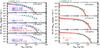 |
Fig. 1 Molecular gas mass function of Herschel galaxies. Left: comparison of the 1/Va estimate (green squares, based on Eq. (1)) with literature data (Keres et al. 2003) and models (Obreschkow & Rawlings 2009a; Lagos et al. 2011; Duffy et al. 2012). The red line and shaded area at z = 1.0−2.0 are obtained by scaling the Muzzin et al. (2013) stellar mass function using the molecular gas fractions reported by Tacconi et al. (2013). When needed, masses found in the literature were scaled by the factor 1.36 necessary to account for helium, and were matched to our set of cosmological parameters. Right: results of the parametric STY evaluation of a Schechter mass function (red lines) and its 3σ uncertainty (shaded areas). |
The comoving number density of galaxies in intervals of Mmol was computed adopting the well-known 1/Va formalism:  (2)where the sum is computed over all sources in the given Mmol bin. The accessible volume Va is a spherical shell delimited by
  and
and  . Here zmax is the highest redshift at which a galaxy would be observable in our survey (Schmidt 1968), and
  define redshift bins.
Our source selection was mainly based on a 160 μm cut, and the UV requirements do not produce significant source losses. On the other hand, the conversion from S(160) to L(IR) was obtained by adopting a family of SED templates spanning a variety of colors. Moreover, UV properties are also involved in computing the total SFR and in applying Eq. (1).
As a consequence, the conversion between the 160 μm fluxes and molecular gas mass is not unique, but comprises a distribution of mass-to-light ratios. Because of this scatter in Mmol vs. S(160), a flux cut induces a molecular mass incompleteness. This effect was thoroughly studied by Fontana et al. (2004) and Berta et al. (2007), among others, for stellar mass. Equivalently, the recipe defined by these authors can be applied to the specific case of molecular gas mass and FIR fluxes to derive completeness corrections as a function of Mmol. Using the distribution of the parent MS population and comparing it with that of PACS galaxies leads to similar results.
The comoving number density of galaxies is shown in Fig. 1. Results from the τdep scaling or Eq. (1) are very similar, thus only the latter are shown. Table 1 reports the two estimates, along with average completeness values for each mass bin, which also includes the photometric completeness of the FIR catalogs.
An independent characterization of the mass function is provided by the maximum-likelihood approach by Sandage et al. (1979, STY). We adopted the Bayesian implementation by Berta et al. (2007) and adapted it to our case, thus fully propagating the actual Mmol uncertainties into the parametric function evaluation. The adopted functional form to describe the mass function is a Schechter (1976) function:  (3)where Φ ∗ represents the normalization, α the slope in the low-mass regime, and M ∗ the transition mass between a power-law and the exponential drop-off, and the e-folding mass of the latter. Berta et al. (2007) provided more details about this method. Table 2 includes the most probable parameter values and their 3σ uncertainties, obtained with both Mmol estimates. The right-hand panel of Fig. 1 compares the result of the STY analysis with the 1/Va mass function. No STY analysis was attempted for the highest redshift bin because only the very massive end is covered.
The Schechter M ∗ parameter increases by more than a factor of 3 between z = 0.4 and 0.8, and then flattens at z > 1. This rate resembles the evolution of the IR luminosity function of normal star-forming galaxies (Gruppioni et al. 2013) and reflects the link between SFR and Mmol. At the same time, Φ ∗ varies by only a factor of 2 over the 0.4–1.5 redshift range. The net effect is a significant evolution of the number density of galaxies with large Mmol, while at the low-mass end it remains roughly constant. Finally, the most probable value of α steepens as redshift increases, but this might be simply an effect of the different mass ranges effectively constrained at different redshifts (note that the 3σ confidence levels are consistent with nearly no evolution).
We compared this Mmol mass function with an estimate based on stellar mass. Using the PHIBSS CO survey, Tacconi et al. (2013, see their Fig. 12) computed molecular gas fractions for z = 1.0−1.5 normal star-forming galaxies as a function of M ⋆ . We combined these gas fractions with the z = 1.0−1.5 stellar mass function of star-forming galaxies by Muzzin et al. (2013, see also Ilbert et al. 2013; Drory et al. 2009. To account for the MS width in this estimate, we applied a 0.2 dex Gaussian smoothing. The result is close to the observed mass function at z = 1.0−2.0 (Fig. 1). Note also the related approach of Sargent et al. (in prep.), as quoted in Carilli & Walter (2013).
4. Discussion
Our observed Mmol function was computed only for normal star-forming galaxies within ± 0.5 dex in SFR from the main sequence. Thus it represents a lower limit to the total Mmol mass function, by missing passive (low SFR) galaxies and powerful, above-sequence objects. Passive galaxies will provide a negligible contribution unless they include a hypothetical population of molecular gas-rich galaxies forming stars with very low efficiency. For reference, local passive galaxies, lying at Δ(sSFR)MS ≤ −1.0 dex, have molecular gas fractions fmol ≤ 2% (Saintonge et al. 2012). Star-bursting galaxies, i.e., those lying above the MS, should play only a minor role in shaping the mass function as well Rodighiero et al. (2011) have shown that the contribution of above-sequence sources to the number density of star-forming galaxies and total SFR density at z = 1.5−2.5 is low. For our Δlog (SFR)MS = 0.5 cut, we found that objects above the MS contribute no more than ~4% to the number density of star-forming galaxies and ~16% to their SFR density. Depending on whether galaxies rise above the main sequence mostly due to an increased star formation efficiency at fixed gas mass or due to larger gas masses, the effect on the mass function will vary between a global upward ~4% shift or a preferential increase at higher gas masses within the limits permitted by the 16% SFR contribution. Saintonge et al. (2012) showed that in local starbursts the two effects share a 50%–50% role in causing SFR changes with respect to the MS.
Our results are compared in Fig. 1 with the Keres et al. (2003) local CO mass function of IRAS-selected galaxies. Applying a variable CO-to-H2 conversion factor, inversely dependent on L(CO) itself, Obreschkow & Rawlings (2009b,a) obtained a revisited mass function that quickly drops at the high-mass end. Modeling was implemented by post-processing the De Lucia & Blaizot (2007) semi-analytic (SAM) results and assigning the atomic and molecular gas content to galaxies via a set of physical prescriptions (see Obreschkow et al. 2009). Their expectations (Fig. 1) tend to predict a too steep mass function at both low and high redshift. A second model based on the SAM approach was developed by Lagos et al. (2011), starting from the Bower et al. (2006) galaxy formation model. As in Obreschkow & Rawlings (2009a), the Blitz & Rosolowsky (2006) star formation law was adopted, but in this case it was implemented throughout the galaxy evolution process in the SAM model. The model was tested against the observed stellar mass density evolution and the atomic and molecular gas content of local galaxies. Results are shown in Fig. 1, and are now much closer to our observed mass function up to z ~ 2. Figure 1 finally includes predictions of the hydrodynamical simulation developed by Duffy et al. (2012), which overall tend to overestimate the mass function, but are consistent with data at the observed high-mass tail.
Adopting the STY Schechter results, we integrated the mass function from 107 M⊙ to infinity and obtained a measure of the molecular gas mass density (see Table 2 and top panel of Fig. 2). A second estimate obtained by limiting the integral to the mass range effectively covered by observations is also provided. The molecular gas mass density increases by a factor of ~4 from z = 0 to z = 1 and then remains almost constant up to z ~ 2. For reference we plot also the M ⋆ density (Muzzin et al. 2013; Ilbert et al. 2013) up to z = 4. The different trends reflect the growth of gas fractions as a function of redshift (e.g., Tacconi et al. 2013).
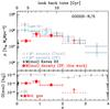 |
Fig. 2 Top: redshift evolution of the molecular gas mass density based on Eq. (1). Red symbols and solid error bars belong to the total mass density, dashed error bars mark lower limits limited to the mass range covered by observations. The black star is computed by integrating the local mass function (Keres et al. 2003). Gray squares and triangles represent the total M ⋆ density reported by Ilbert et al. (2013) and Muzzin et al. (2013), respectively. Light-blue symbols belong to star-forming galaxies only. Bottom: evolution of Ωmol (red symbols, this work) and ΩHI (Prochaska & Herbert-Fort 2004; Zwaan et al. 2005; Rao et al. 2006), where we have divided the latter by 1.3 to avoid counting helium twice. |
Finally, we computed the redshift evolution of the density parameter Ωmol(z) = ρmol(z)/ρc(z) (Fig. 2 and Table 2), where the critical density at the given redshift is given by  . The molecular gas density parameter peaks at z ~ 1.0; for comparison ΩHI, derived from damped Ly-α systems (Prochaska & Herbert-Fort 2004; Rao et al. 2006), and including also low column density cases, does not evolve between z = 0.5 and 4.0.
Using the deepest Herschel extragalactic observations available and restframe UV information for roughly 700 main-sequence galaxies, we have built the first molecular gas mass function at redshift z > 0 and the first estimate of its density evolution up to z = 3. While future mm/submm surveys will significantly improve our knowledge of the molecular content in high-z galaxies, we have provided a basis for refinement of galaxy evolution models that are accounting for the molecular phase.
Acknowledgments
PACS has been developed by a consortium of institutes led by MPE (Germany) and including UVIE (Austria); KU Leuven, CSL, IMEC (Belgium); CEA, LAM (France); MPIA (Germany); INAF-IFSI/OAA/OAP/OAT, LENS, SISSA (Italy); IAC (Spain). This development
has been supported by the funding agencies BMVIT (Austria), ESA-PRODEX (Belgium), CEA/CNES (France), DLR (Germany), ASI/INAF (Italy), and CICYT/MCYT (Spain).
References
- Berta, S., Lonsdale, C. J., Polletta, M., et al. 2007, A&A, 476, 151 [NASA ADS] [CrossRef] [EDP Sciences] [Google Scholar]
- Berta, S., Magnelli, B., Nordon, R., et al. 2011, A&A, 532, A49 [NASA ADS] [CrossRef] [EDP Sciences] [Google Scholar]
- Berta, S., Lutz, D., Santini, P., et al. 2013, A&A, 551, A100 [NASA ADS] [CrossRef] [EDP Sciences] [Google Scholar]
- Blitz, L., & Rosolowsky, E. 2006, ApJ, 650, 933 [NASA ADS] [CrossRef] [Google Scholar]
- Bouché, N., Dekel, A., Genzel, R., et al. 2010, ApJ, 718, 1001 [NASA ADS] [CrossRef] [Google Scholar]
- Bower, R. G., Benson, A. J., Malbon, R., et al. 2006, MNRAS, 370, 645 [NASA ADS] [CrossRef] [Google Scholar]
- Carilli, C., & Walter, F. 2013 [arXiv:1301.0371] [Google Scholar]
- Chabrier, G. 2003, PASP, 115, 763 [NASA ADS] [CrossRef] [Google Scholar]
- Daddi, E., Dickinson, M., Morrison, G., et al. 2007, ApJ, 670, 156 [NASA ADS] [CrossRef] [Google Scholar]
- Davé, R., Finlator, K., Oppenheimer, B. D., et al. 2010, MNRAS, 404, 1355 [NASA ADS] [Google Scholar]
- De Lucia, G., & Blaizot, J. 2007, MNRAS, 375, 2 [NASA ADS] [CrossRef] [Google Scholar]
- Drory, N., Bundy, K., Leauthaud, A., et al. 2009, ApJ, 707, 1595 [NASA ADS] [CrossRef] [Google Scholar]
- Duffy, A. R., Kay, S. T., Battye, R. A., et al. 2012, MNRAS, 420, 2799 [NASA ADS] [Google Scholar]
- Elbaz, D., Daddi, E., Le Borgne, D., et al. 2007, A&A, 468, 33 [NASA ADS] [CrossRef] [EDP Sciences] [Google Scholar]
- Elbaz, D., Dickinson, M., Hwang, H. S., et al. 2011, A&A, 533, A119 [NASA ADS] [CrossRef] [EDP Sciences] [Google Scholar]
- Fontana, A., Pozzetti, L., Donnarumma, I., et al. 2004, A&A, 424, 23 [NASA ADS] [CrossRef] [EDP Sciences] [Google Scholar]
- Fukugita, M., Hogan, C. J., & Peebles, P. J. E. 1998, ApJ, 503, 518 [NASA ADS] [CrossRef] [Google Scholar]
- Grazian, A., Fontana, A., de Santis, C., et al. 2006, A&A, 449, 951 [NASA ADS] [CrossRef] [EDP Sciences] [Google Scholar]
- Gruppioni, C., Pozzi, F., Rodighiero, G., et al. 2013, MNRAS, 432, 23 [NASA ADS] [CrossRef] [Google Scholar]
- Ilbert, O., McCracken, H. J., Le Fevre, O., et al. 2013, A&A, in press, 10.1051/0004-6361/201321100 [Google Scholar]
- Kennicutt, Jr., R. C. 1998, ARA&A, 36, 189 [Google Scholar]
- Keres, D., Yun, M. S., & Young, J. S. 2003, ApJ, 582, 659 [NASA ADS] [CrossRef] [Google Scholar]
- Lagos, C. D. P., Baugh, C. M., Lacey, C. G., et al. 2011, MNRAS, 418, 1649 [NASA ADS] [CrossRef] [Google Scholar]
- Lilly, S. J., Carollo, C. M., Pipino, A., Renzini, A., & Peng, Y. 2013 [arXiv:1303.5059] [Google Scholar]
- Lutz, D., Poglitsch, A., Altieri, B., et al. 2011, A&A, 532, A90 [NASA ADS] [CrossRef] [EDP Sciences] [Google Scholar]
- Magdis, G. E., Daddi, E., Elbaz, D., et al. 2011, ApJ, 740, L15 [Google Scholar]
- Magdis, G. E., Daddi, E., Béthermin, M., et al. 2012, ApJ, 760, 6 [NASA ADS] [CrossRef] [Google Scholar]
- Magnelli, B., Elbaz, D., Chary, R. R., et al. 2011, A&A, 528, A35 [Google Scholar]
- Magnelli, B., Popesso, P., Berta, S., et al. 2013, A&A, 553, A132 [NASA ADS] [CrossRef] [EDP Sciences] [Google Scholar]
- Meurer, G. R., Heckman, T. M., & Calzetti, D. 1999, ApJ, 521, 64 [NASA ADS] [CrossRef] [Google Scholar]
- Muzzin, A., Marchesini, D., Stefanon, M., et al. 2013, ApJS, 206, 8 [Google Scholar]
- Noeske, K. G., Weiner, B. J., Faber, S. M., et al. 2007, ApJ, 660, L43 [Google Scholar]
- Nordon, R., Lutz, D., Genzel, R., et al. 2012, ApJ, 745, 182 [NASA ADS] [CrossRef] [Google Scholar]
- Nordon, R., Lutz, D., Saintonge, A., et al. 2013, ApJ, 762, 125 [NASA ADS] [CrossRef] [Google Scholar]
- Obreschkow, D., & Rawlings, S. 2009a, ApJ, 696, L129 [NASA ADS] [CrossRef] [Google Scholar]
- Obreschkow, D., & Rawlings, S. 2009b, MNRAS, 394, 1857 [NASA ADS] [CrossRef] [Google Scholar]
- Obreschkow, D., Croton, D., De Lucia, G., Khochfar, S., & Rawlings, S. 2009, ApJ, 698, 1467 [NASA ADS] [CrossRef] [Google Scholar]
- Pilbratt, G. L., Riedinger, J. R., Passvogel, T., et al. 2010, A&A, 518, L1 [CrossRef] [EDP Sciences] [Google Scholar]
- Poglitsch, A., Waelkens, C., Geis, N., et al. 2010, A&A, 518, L2 [NASA ADS] [CrossRef] [EDP Sciences] [Google Scholar]
- Prochaska, J. X., & Herbert-Fort, S. 2004, PASP, 116, 622 [NASA ADS] [CrossRef] [Google Scholar]
- Rao, S. M., Turnshek, D. A., & Nestor, D. B. 2006, ApJ, 636, 610 [NASA ADS] [CrossRef] [Google Scholar]
- Rodighiero, G., Daddi, E., Baronchelli, I., et al. 2011, ApJ, 739, L40 [NASA ADS] [CrossRef] [Google Scholar]
- Saintonge, A., Kauffmann, G., Kramer, C., et al. 2011, MNRAS, 415, 32 [NASA ADS] [CrossRef] [Google Scholar]
- Saintonge, A., Tacconi, L. J., Fabello, S., et al. 2012, ApJ, 758, 73 [Google Scholar]
- Sandage, A., Tammann, G. A., & Yahil, A. 1979, ApJ, 232, 352 [NASA ADS] [CrossRef] [EDP Sciences] [Google Scholar]
- Santini, P., Fontana, A., Grazian, A., et al. 2009, A&A, 504, 751 [NASA ADS] [CrossRef] [EDP Sciences] [Google Scholar]
- Schechter, P. 1976, ApJ, 203, 297 [Google Scholar]
- Schmidt, M. 1968, ApJ, 151, 393 [NASA ADS] [CrossRef] [Google Scholar]
- Scoville, N. Z. 2012 [arXiv:1210.6990] [Google Scholar]
- Tacconi, L. J., Neri, R., Genzel, R., et al. 2013, ApJ, 768, 74 [Google Scholar]
- Teplitz, H. I., Chary, R., Elbaz, D., et al. 2011, AJ, 141, 1 [NASA ADS] [CrossRef] [Google Scholar]
- Wuyts, S., Förster Schreiber, N. M., Lutz, D., et al. 2011, ApJ, 738, 106 [NASA ADS] [CrossRef] [Google Scholar]
- Zwaan, M. A., Meyer, M. J., Staveley-Smith, L., & Webster, R. L. 2005, MNRAS, 359, L30 [NASA ADS] [CrossRef] [Google Scholar]
All Tables
All Figures
|
Fig. 1 Molecular gas mass function of Herschel galaxies. Left: comparison of the 1/Va estimate (green squares, based on Eq. (1)) with literature data (Keres et al. 2003) and models (Obreschkow & Rawlings 2009a; Lagos et al. 2011; Duffy et al. 2012). The red line and shaded area at z = 1.0−2.0 are obtained by scaling the Muzzin et al. (2013) stellar mass function using the molecular gas fractions reported by Tacconi et al. (2013). When needed, masses found in the literature were scaled by the factor 1.36 necessary to account for helium, and were matched to our set of cosmological parameters. Right: results of the parametric STY evaluation of a Schechter mass function (red lines) and its 3σ uncertainty (shaded areas). |
| In the text | |
|
Fig. 2 Top: redshift evolution of the molecular gas mass density based on Eq. (1). Red symbols and solid error bars belong to the total mass density, dashed error bars mark lower limits limited to the mass range covered by observations. The black star is computed by integrating the local mass function (Keres et al. 2003). Gray squares and triangles represent the total M ⋆ density reported by Ilbert et al. (2013) and Muzzin et al. (2013), respectively. Light-blue symbols belong to star-forming galaxies only. Bottom: evolution of Ωmol (red symbols, this work) and ΩHI (Prochaska & Herbert-Fort 2004; Zwaan et al. 2005; Rao et al. 2006), where we have divided the latter by 1.3 to avoid counting helium twice. |
| In the text | |
Current usage metrics show cumulative count of Article Views (full-text article views including HTML views, PDF and ePub downloads, according to the available data) and Abstracts Views on Vision4Press platform.
Data correspond to usage on the plateform after 2015. The current usage metrics is available 48-96 hours after online publication and is updated daily on week days.
Initial download of the metrics may take a while.