| Issue |
A&A
Volume 554, June 2013
|
|
|---|---|---|
| Article Number | A116 | |
| Number of page(s) | 10 | |
| Section | The Sun | |
| DOI | https://doi.org/10.1051/0004-6361/201321259 | |
| Published online | 13 June 2013 | |
Empirical determination of the temperature stratification in the photosphere of the quiet Sun
UMR 7293 Lagrange Laboratory, Université de Nice Sophia Antipolis, CNRS, Observatoire de la Côte d’Azur, Campus Valrose, 06108 Nice, France
e-mail: This email address is being protected from spambots. You need JavaScript enabled to view it.
; This email address is being protected from spambots. You need JavaScript enabled to view it.
; This email address is being protected from spambots. You need JavaScript enabled to view it.
Received: 7 February 2013
Accepted: 17 April 2013
Abstract
Context. Detailed realistic 3D simulations of the photosphere of the Sun are now available, but 1D models of the average quiet-Sun photosphere are still widely used, in particular for spectro-polarimetric inversions.
Aims. Here we present an empirical determination of the average radiation temperature variations as a function of the geometrical height above the continuum formation level in the solar photosphere.
Methods. We used high resolution spectroscopic scans in the 630 nm Fe i line pair at varying heliocentric angles along the north-south polar axis of the Sun, made with SOT onboard Hinode. Implementing a new method for image reconstruction, we obtained images of the photospheric granulation at constant continuum opacity levels, from the upper photosphere seen at line centers to the low photosphere. The Fourier cross-spectra of images at different opacity levels were computed, and we derived the formation depths of images without referring to any atmospheric model, by measuring the slope of the cross-spectrum phase.
Results. A modified Milne-Eddington model for the line formation was tested by comparing it with the average line-intensity profiles observed at solar disk center. It yields consistent results for the FeI 630.2 nm line, whereas the FeI line at 630.1 nm is not well reproduced by the model. We ascribe this discrepancy to non-LTE effects in the line formation processes. The average image intensities at the different FeI 630.2 nm levels were used to determine the depth-variation of the temperature for an average 1D model of the quiet photosphere. We compared our empirical temperature model with the widely used FALC model. Both models agree well for the temperature variations with the continuum optical depth. But in the low photosphere, the temperature gradient we measure with respect to the geometrical height is significantly softer than in Model C. We argue that some of the assumptions used to solve the pseudohydrostatic equilibrium in semi-empirical models are probably at fault. We also derived empirical values for the 630 nm continuum absorption coefficient as a function of the geometrical height in the low photosphere. Finally, we were able to measure the altitude of the base of the granulation contrast inversion layer, which is found at about 130 km above the base of the photosphere, in agreement with 3D MHD simulations.
Key words: line: formation / techniques: high angular resolution / techniques: spectroscopic / Sun: photosphere
© ESO, 2013
1. Introduction
Usually, semi-empirical modeling of the solar photosphere consists of adjusting the temperature stratification as a function of gas pressure in such a way that the computed intensities match the observed disk center intensities and center-to-limb variation (CLV) at various wavelengths. They thus require one to solve the radiative transfer equation in lines and continua in prescribed temperature-density hydrostatic equilibrium models. The most up-to-date model for the quiet-Sun photosphere was presented as Model C in Fontenla et al. (2006). It is based on the previous Model C of Maltby et al. (1986) that was modified to account for new observations and improved values of atomic data. Here we present a fully empirical derivation of the radiation temperature stratification in the average quiet Sun, which does not rely on any radiative transfer computation.
Using Hinode/SOT spectroscopic scans of the quiet-Sun photosphere in the FeI 630 nm line pair, we implemented the line-cord method introduced in Faurobert et al. (2012) to reconstruct images of the photosphere at 25 continuum opacity levels, ranging from the continuum formation layer (level 25) to the upper layers, where the line cores are formed. In the second section of this paper we briefly recall the line-cord method and present the center-to-limb variations of the average intensity of the images at each line-cord level. Then we test the validity of a modified Milne-Eddington model for reproducing the average intensities observed at disk center as functions of the line-cord level, assuming local thermodynamic equilibrium (LTE). For the images obtained in the FeI 630.2 nm line, the intensities predicted by the model are consistent with the observations, whereas for the stronger FeI 630.1 nm line, some discrepancies appear in the line core, probably because of non-LTE effects in the line formation processes. The LTE Milne-Eddington model or a simple Eddington-Barbier approximation may be used to derive empirical values of the continuum opacity at the 25 line-cord levels in the FeI 630.2 nm line and in the wings of the FeI 630.1 nm line.
In the third part, we implement a cross-spectral method previously introduced in Grec et al. (2007, 2010) to measure the altitude where the line-cord images are formed. It is based on the following ideas: when two images at different wavelengths are observed out of disk center, the perspective effect due to their formation height difference yields a systematic shift between the images projected in the plane of the sky. If the two images are similar enough, this shift is detected as a linear term in the phase of their Fourier cross-spectrum. By measuring the slope of the cross-spectrum phase term we obtain a model-independent measurement of the geometrical heights of the image-forming layers. In Faurobert et al. (2009) the method was successfully applied to images obtained with Hinode/SOT in the line cores of the FeI 630 nm line pair, and yielded the depth difference between the line core formation depths. In Faurobert et al. (2012) we used a cross-correlation method to determine the altitudes where the line centers are formed. We showed that the cross-correlation between continuum and line center images shows a negative peak because of the contrast inversion of the granulation seen at line centers. The measurement of the perspective displacement of the negative peak, observed out of disk center, allowed us to determine the line center formation heights.
Cross-spectral and cross-correlation methods are quite complementary. The cross-correlation method takes advantage of the granulation contrast inversion between the continuum and the line center forming layers, whereas the cross-spectral method relies on the assumption that the images seen at different line-cords are similar enough, which does not allow us to measure depth-differences between images formed below and above the contrast inversion layer. In this paper we apply the cross-spectral method to determine the formation heights of the line-cord levels formed below the contrast inversion layer with respect to the 630 nm continuum formation depth, and the depth of line-cord levels formed above the inversion layer with respect to the line center formation height. The formation heights of line-cord levels formed within the contrast inversion layer cannot be measured properly. We are nevertheless able to recover the overall depth-gradient of the radiation temperature in the photosphere between 0 and 250 km above the continuum formation level, and we precisely measure its depth-gradient in the low photosphere, between 20 and 120 km. We compare our empirical results to the widely used Model C presented in Fontenla et al. (1999, 2006).
2. Center-to-limb variations of the mean intensity in the line-cord images
We used high resolution spectroscopic scans of the granulation obtained in the FeI 630 nm line pair with SOT onboard Hinode, on December 19, 2007. The 1024 pixel-spectrograph slit parallel to the north-south polar axis of the Sun was successively located at 20 latitudes allowing us to continously scan the full center-to-limb variations of the solar disk image. At each location a 380-step west-est scan was performed, with a step size of 0.16 arcsec. The pixel size along the slit is 0.16 arcsec, which limits the spatial resolution of the images to 0.32 arcsec (the diffraction limit of the 50-cm miror of the telescope is 0.24 arcsec in the visible domain at 630 nm, the images are thus slightly undersampled by the SOT/SP cameras). We recall that on December 19 the geometrical distance on the Sun surface, seen under one arcsecond, is 714 km. Because each 380 × 1024 image covers a large part (164 arcsec) of the solar diameter, we divided it into eight 380 × 128 images (60.8′′ × 20′′), where we assumed that the value of the heliocentric angle remains approximately constant (we considered its value at the central pixel). The spectral resolution of the SOT spectrograph is 2.15 pm/px in our spectral domain between 630.08 and 630.32 nm. The observational data we analyzed consist of (380 × 128) images at 160 successive heliocentric angles along the solar diameter and at 112 wavelengths scanning both lines.
2.1. Line-cord method for image reconstruction
When observations are performed in a spectral line, the opacity varies steeply with the wavelength. It is given by  (1)where kc is the continuum opacity, kl is the frequency-averaged line opacity, λ0 is the line center wavelength in the observer’s frame, and φ is the normalized absorption profile, which typically goes to zero on a Doppler width scale ΔλD. The Doppler broadening is due both to thermal broadening and to unresolved velocities. It is important to notice here that we assumed that φ is a function of the “reduced” wavelength variable δλ = (λ − λ0)/ΔλD, depending both on the line center wavelength and on the Doppler width. We did not account for broadening due to damping effects, which could be significant in the wings of strong lines. This assumption is valid for the FeI line pair at 630 nm.
In Faurobert et al. (2012) we have implemented a method that allows us to recover images formed in layers located at constant continuum optical depths. Introducing the line strength r = kl/kc, the opacity at a wavelength λ is written k(λ) = kc(1 + rφ(δλ)). To recover the photospheric structures at given continuum opacity levels from the spectroscopic scans, we have to build images at constant values of (1 + rφ(δλ)) over the observed solar surface.
Line-of-sight velocities due to granular motions and to 5-mn oscillations have two effects on the line absorption profile. The line center wavelength λ0 is shifted, and unresolved line-of-sight velocities and/or their depth-gradients affect the observed line width and the line asymmetry. These two physical effects lead to variations of the opacity k(λ) at a given λ value over the solar surface. Furthermore, variations of temperature and density due to the presence of structures also modify the local Doppler width and the line strength r. In Faurobert et al. (2012) we considered 25 evenly distributed line cords Δλi, defined by Δλi/Δλc = i/24, where the index i varies from 0 at line center to 24, and Δλc is the line-cord width measured close to the continuum level (namely where the line residual intensity is 98% of the continuum intensity), and we built 25 images for each scan position on the solar disk by extracting the residual line intensity at these line cords. We stress that the line cords Δλi are not constant over the image because Δλc varies from pixel to pixel, but the reduced cord grid δλ = Δλi/Δλc, which is the relevant quantity as far as the opacity is concerned, is uniform over the image (see Faurobert et al. (2012) for a more detailed presentation of the method).
2.2. Mean line-cord image intensities
The measurements of the mean image intensity at the different line-cord levels, normalized to the continuum average intensity at disk center, are shown in Fig. 1 for the 630.15 nm and the 630.25 nm Fe i lines, for μ = cosθ varying between 1 and 0.2, in the southern and northern hemispheres. Closer to the solar limb the value of cosθ varies very fast over a 128 pixel wide image, therefore we were unable to properly measure the average intensity at low μ values. We notice a slight asymmetry between the northern and southern hemispheres (see Fig. 2).
At the continuum level we recover the smooth center-to-limb variation, which may be represented by a fifth-order polynomial in cosθ, as in Neckel (2005), except for some local peaks generated by bright faculae at some locations on the solar disk. The average intensity decreases for images observed at increasing depth in the lines, which is expected since the temperature decreases with height in the photosphere.
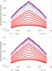 |
Fig. 1 Center-to-limb variations of the mean intensity of the photosphere at 25 line-levels, normalized to the mean intensity of the continuum at disk center. Upper panel: FeI 630.1 nm line; lower panel: FeI 630.2 nm. The right sides of the figures show the measurements performed in the northern hemisphere as functions of 1 − cosθ (0 at disk center), the left sides show the results for the southern hemisphere as funtions of − (1 − cosθ). From the lower curve to the top one the line-cord index varies from 1 to 25 (line center to continuum level). Parabolic fittings (in red) are superimposed to the observed curves at line cords 1 to 9 and 20. The thin smooth line shows the fifth-order polynomial fitting of the continuum mean intensity, as given by Neckel (2005). |
2.3. A modified Milne-Eddington model
According to the widely used Eddington-Barbier approximation, the forming layer of the emerging radiation at a line cord δλ in the direction μ is located at the height where the adjacent continuum optical depth τ ≃ μ/(1 + rφ(δλ)). Accordingly, if the line is formed under LTE conditions, the residual line intensity observed at disk center at a given line cord should be identical to the continuum intensity observed in the direction μ = 1/(1 + rφ(δλ). This allows us to derive an empirical value of the opacity factor 1 + rφ(δλ), simply from the direction μ where the continuum intensity is equal to the residual line intensity observed at disk center. The results of this simple empirical procedure are given in Tables 1 and 2 for the FeI 630.1 nm and 630.2 nm, respectively. We used the continuum CLV derived from our Hinode observations for μ > 0.2 and those reported in Neckel (2005) at lower μ values (they were both normalized to the continuum mean intensity measured at disk center). We notice that the opacity in the first two levels of the FeI 630.1 nm line cannot be obtained from this simple procedure because the line core intensity at disk center is lower than the continuum intensity measured at the solar limb. This is probably a consequence of non-LTE effects in the line formation mechanisms.
The CLV observations presented above may also be used to perform a simple test of the Milne-Eddington model applied to the average line-cord intensities in the FeI 630 nm line pair.
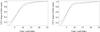 |
Fig. 2 Slope of the mean intensity CLV in the FeI 630.15 nm (left panel) and in the FeI 630.25 nm (right panel) measured at disk center for the 25 line cords, and normalized to 1 at level 25. Values fitting the northern and southern hemisphere measurements are shown in red and in blue, respectively. |
Comparison of the line-cord opacity factors (1 + rφ(δλ)) derived from a Milne-Eddington model (ME) and from the Eddington-Barbier approximation (EB) for the FeI 630.15 nm line.
Same as Table 1 for the FeI 630.2 nm line.
In the Milne-Eddington model, one assumes that the line source function is a linear function of the continuum opacity along the vertical direction (denoted by τ in the following) and that both their strengths with respect to the continuum and their Doppler width are independent of depth. Here we also assumed that the lines are formed in LTE.
Because the Planck function varies according to the physical conditions in the different granular structures, we considered here a so-called 1.5 D representation of the radiative transfer, which amounts in neglecting radiative transport in directions parallel to the solar surface. The 1.5D radiative transfer equation in a spectral line is then written  (2)where x and y denote the coordinates in the plane parallel to the solar surface, δλ is the reduced line cord introduced previously. Following the Milne-Eddington model, we write
  (3)The emerging radiation at line cord δλ, is then given by
  (4)Averaging over x and y, we obtain the expression of the mean continuum-intensity at disk center, namely
  (5)The Milne-Eddington model assumes that rφ(δλ) does not depend on the altitude z, here we may also assume that the quantity 1 + rφ(δλ) is constant over the whole image as explained in the previous section. Then, the mean intensity observed in the line in the direction μ, normalized to the continuum intensity at disk center, is given by
 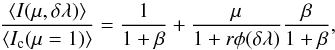 (6)where we have introduced the notation β = ⟨ B1(x,y) ⟨ / ⟨ B0(x,y) ⟨.
 |
Fig. 3 Parameters a and b of the parabolic fits of the mean intensity CLV as functions of the line-cord index. Upper panels: a and b parameters for the FeI 630.1 nm line; lower panels: a and b parameters for the FeI 630.2 nm line. Values measured in the northern and in the southern hemispheres are shown in red and blue, respectively. |
We notice that the average emerging line profiles do not have the same shape as the opacity factor, except if the line strength r < < 1 (weak line) and β/(1 + β) is depth-independent. However, Eq. (6) shows that, in a Milne-Eddington model, the slope of the center-to-limb variations of the mean intensity measured at disk center for a given line cord is related to its opacity factor 1 + rφ(δλ).
This property may be used to derive the opacity factor of the line cords with respect to the continuum opacity. We therefore measured the slope at disk-center of the CLV curves shown in Fig. 1 using a simple finite-difference formula. Some uncertainty on this measurement is caused by the presence of local bright regions close to disk center. We were able to estimate an average value by slightly varying the width of the finite μ interval, because at disk center we have a very fine sampling of the CLV curve, with a large number of images at μ values close to one. We noticed significant differences between slopes measured on the southern side and the northern side of the equator (see Fig. 2). The mean values of the slopes are given in Tables 1 and 2, together with an estimate of the error bar. We remark that the shape of the curves shown on Fig. 2 is reminiscent of the line absorption profile, as expected from Eq. (6). If the coefficient β were a constant quantity at all depths in the photosphere, we would recover exactly the profile of the line opacity with respect to the continuum opacity. But, because we are dealing with quite strong lines that are formed over a broad range of continuum optical depths, it would not be correct to assume that the Planck function is a linear function of τ over this broad domain. Therefore we modified the standard Milne-Eddington model by regarding the depth gradient of the Planck function as a quantity that varies slowly with τ. This means that the residual line intensities, measured at disk center at different line cords, may be derived from the Milne-Eddington model as in Eq. (6), but with the local value of the parameter β in the relevant forming layer, i.e., at τ = 1/(1 + rφ(δλ)). Because this is also the forming layer of the continuum intensity observed at μ = 1/(1 + rφ(δλ)), we derived β/(1 + β) from the slope of the continuum CLV at this μ value.
We determined the continuum CLV slope from our own Hinode observations, shown in Fig. (1) and from the observations reported in Neckel (2005); they both give very close results. But our measurements are limited to μ values higher than 0.2, therefore we chose to use Neckel’s data for the full range of μ.
The values of β/(1 + β) and of the opacity factor 1 + rφ(δλ) are given in Tables 1 and 2 for the line-cord levels 1 to 20 in both lines (the line cords 21 to 25 are very close to the continuum). In the last column we also give, when it is defined, the result of the Eddington-Barbier approximation. For the FeI 630.2 nm line, the differences between the Milne-Eddington model and the Eddington-Barbier approximations are within the error bars of the methods. For the stronger FeI 630.1 nm line, we notice significant discrepancies between the two methods, probably due to non-LTE effects in this line formation process.
The Milne-Eddington model is often used in inversion codes for deriving magnetic field maps from Stokes parameters measured in these lines. The inversion method has been extensively tested in this context (Orozco Suárez et al. 2010). In the inversion procedure the source function linear depth-variations are described by free parameters that are derived from the minimization code at each pixel of the image. It seems to us that the FeI 630.2 nm line is a better candidate for Milne-Eddington inversion procedures than the stronger (but less sensitive to magnetic fields) FeI 630.1 nm line.
2.4. Quadratic fits of the center-to-limb variations
We found that the CLV of the mean intensities in line-cord images, normalized to the continuum disk center intensity, are well represented by quadratic polynomial functions of (1 − μ) of the form a(1 − μ)2 + b(1 − μ) + c. The a and b coefficients were derived from least-square-fitting of the observed curves. To take into account the asymmetry of the CLV with respect to the equator, we performed separate fittings on the northern and southern hemispheres. The behavior of the coefficients a and b as functions of the line-cord index is shown on Fig. 3. The values of c are given in Tables 1 and 2. There is a north-south asymmetry in both a and b.
3. Radiation-temperature stratification
In this section we implement the cross-spectral method previously introduced in Grec et al. (2007) and tested numerically in Grec et al. (2010). It allows us to measure the depth-difference between two image formation layers without referring to any atmospheric model. This yields an empirical determination of the relationship between geometrical heights and the continuum optical depth scale, avoiding the solution of the hydrostatic equilibrium equation. We first briefly recall the main steps of the cross-spectral method.
3.1. Cross-spectral method
The image obtained at a line-cord level i, denoted by Ii(x,y), is formed higher in the photosphere than the continuum image Ic(x,y). Because of the perspective effect, Ii(x,y) will appear to be shifted toward the limb in comparison with Ic(x,y) when the images are observed out of disk center. If we assume that the structures in both images are similar, we can write 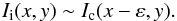 (7)By using for the Fourier transform, the definition
 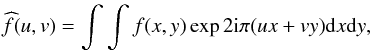 (8)relation (7) becomes in the Fourier space
 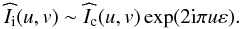 (9)The perspective displacement introduces a deterministic linear phase-term 2πεu, proportional to the angular frequency u.
Because we use spectrograms, we have only access to the 1D brightness intensity along the slit, which is aligned with the x-axis. We thus obtain the value of Ii(x,y) for a fixed y = y0. Two-dimensional images are not needed here, as the spectrograph slit is orientated along the direction of the perspective shift. However, scanning the solar surface allows us to record many spectrograms at differenty positions to improve the statistics of the solar granulation power spectrum. Denoting for simplicity Ii(x) the 1D cuts Ii(x,0) of the images, we can write  (10)and
  (11)Shifts can then be derived from the phase of the cross-spectrum. We used a series of spectrograms to estimate the cross-spectrum
  between Ic(x) and Ii(x):
  (12)where
  represents the conjugate Fourier transform of Ii(x), and the brackets refer to the ensemble average.
We stress that one important assumption here is image similarity. This does not hold when one compares images in the deep line-cores to continuum images. In Grec et al. (2010) we showed that it is possible however to apply the cross-spectral method to images obtained at successive levels in the line, and to obtain the total depth difference between the continuum and any level in the line by simply adding the depth differences between two successive levels.
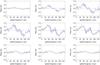 |
Fig. 4 Phase (in radian) of the cross-spectrum of images at successive levels in the FeI 630.1 nm, measured at μ = 0.776 as a function of the spatial frequency given in pixel units. The frequency zero is at pixel 65. Upper row, from left to right: cross-spectra of images at levels 1 and 2, 2 and 3, and 3 and 4. Middle row, from left to right: cross-spectra of images at levels 4 and 5, 5 and 6, 6 and 7 (note the effect of contrast inversion), lower row, from left to right: cross-spectra of images at levels 11 and 12, 12 and 13, 13 and 14. |
3.2. Contrast inversion and cross-spectrum phase
We applied the method recalled in the previous section to images at successive levels in the FeI 630 nm lines. Figure 4 shows the behavior of the cross-spectrum phase for images at successive levels in the FeI 630.1 nm line at μ = 0.776. We notice that the phase has an overall linear behavior (but remark that it may be quite noisy), as long as the two images are both below or above the contrast inversion layer, but exhibit quite a different behavior, with a change of slope of the phase at low frequencies, when the images are formed within the contrast inversion layer. In the following we propose a numerical experiment to model this behavior.
3.2.1. Numerical experiment
We considered a (256 × 256) image of the granulation observed at disk center in the continuum and computed its Fourier spatial spectrum. This reference image contains all the complex photospheric structures. Then we applied a low-pass Gaussian filter on the image spectrum to separate it into a low and a high spatial frequency component. The width of the Gaussian filter is (1./1.3) arcsec-1, so the low-frequency component contains the structures that are larger than the typical granular scale (the supergranular pattern for example). The high-frequency component is simply obtained by subtracting the low-frequency spectrum from the reference image spectrum. We notice that contrast inversion appears at the granular scale but does not affect the low spatial frequency component. Therefore we created an artificial image by shifting the low-frequency component to mimic the perspective effect and by shifting the high -requency component in the opposite direction, to mimic the perspective effect and contrast inversion. Then we computed the cross-spectrum of this simulated image with our reference image. Figure 5 shows the cross-spectrum phase. Its non-linear behavior is very similar (except for a lower noise level) to what we observe in our real data. This experiment illustrates that in the contrast inversion layer, the large-scale structures tend to decouple from the structures at granular scales, and the interplay between contrast inversion at granular scales and the perspective effect leads to the non-linear behavior of the cross-spectrum phase, with two different regimes at low and high spatial frequencies.
The information on the displacement of the low-frequency component is still contained in the phase slope at low frequencies. However, in most real cases the noise level in the image spectrum is too high to allow a meaningful measurement of the phase slope. The slopes of the phase measured by linear fitting in intervals of various widths are shown on Fig. 5 to illustrate the difficulty of such a measurement. In these cases we simply set the phase slope to zero. As a consequence, we were unable to measure the width of the contrast inversion layer and we underestimated the formation heights of line levels in the line cores that are formed above this layer. We shall explain in the following how we could overcome this problem and correct the formation heights of line-core levels for this effect.
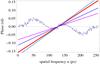 |
Fig. 5 Phase of the cross-spectrum of an image observed in the continuum and a numerically displaced image with a contrast inversion at high spatial frequencies. The red linear curve shows the phase corresponding to the imposed displacement of 0.05 pixel. The spatial frequency zero is at pixel 129. The cyan, blue, and magenta lines show how the measured slope would vary according to the width of the linear fitting interval at the origin, namely ±5 pixels, ±15 pixels and ±25 pixels, respectively. |
3.3. Line-cord formation heights
To obtain the line-cord formation heights we simply added the measured displacements between two successive levels, starting from the continuum level (level 25). Figure 6 shows the center-to-limb variations of the height measured between the continuum level and four different line levels in the FeI lines at 630.1 nm and 630.2 nm (the perspective shift was divided by sinθ to correct for the projection effect). The perspective shift can be measured for lines of sight with μ between 0.20 and 0.87. Closer to the limb, μ varies too rapidly over the image, whereas closer to disk center the perspective effect is too small with respect to the noise level in the cross-spectrum phase. We observe that the line levels in the 630.2 nm line are formed at lower heights than the corresponding ones in the 630.1 nm line. This is expected since the 630.2 nm line is weaker than the 630.1 nm one. The formation heights measured in the line cores (levels 1 and 5) show a higher dispersion than those measured in the line wings. We suspect that this is due to the effect of quiet-Sun magnetic network elements that we observe in the images and that affect the line formation by broadening the line profile and by weakening the lines. Despite a quite high dispersion of the measurements in the line cores, we observe that the formation heights remain roughly independent of μ for μ > 0.7. They are also almost symmetrical in the northern and southern hemispheres. We can thus increase the accuracy of our measurements by averaging the results obtained in both hemispheres at μ > 0.7.
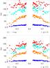 |
Fig. 6 Perspective shifts measured between the continuum and images at four line levels as function of 1 − μ in the northern hemisphere, and − (1 − μ) in the southern hemisphere. Upper panel: results for the Fe1 630.1 nm line. Lower panel: results for the Fe2 630.2 nm. Red dots: line centers (level 1), light -blue dots: level 5, orange dots: line level 10, deep-blue dots: level 15. |
Figure 7 shows the averaged formation heights as a function of the line-cord levels in the FeI 630.1 nm and 630.2 nm lines. We notice that the slope of the curves shows a discontinuous change at line cords between 7 and 8. This is due to the difficulties of the measurements in the contrast inversion layer where these line levels are formed.
However, we observe that the measurements performed in the two lines agree as far as the altitude of the base of the contrast inversion layer is concerned. It is located around z = 110 km above the 630 nm continuum-formation height. According to LTE calculations of the continuum opacities, we find that our reference continuum at λ = 630 nm forms at z = 21 km above the 500 nm continuum which is the standard reference of solar models. This means that we measure the altitude of the base of the granulation contrast inversion layer around 130 km above the standard base of the photosphere. This agrees well with the 3D MHD numerical simulations of Cheung et al. (2007), who found that the base of the contrast inversion layer is between 130 km and 140 km.
Tables 3 and 4 give the radiation temperature at the successive line-cord levels, together with the line-cord formation heights obtained by averaging our measurements for μ > 0.7. As noticed in the previous section, the heights measured in the line cores are underestimated because of the problems we encountered to measure the cross-spectrum phase slope in the contrast inversion layer. In Faurobert et al. (2012) we were able to directly measure the line-core formation heights with a cross-correlation method; we found that the FeI 630.1 nm and FeI 630.2 nm line centers are formed at z = 230 km and z = 200 km above the 630 nm continuum formation height. Comparing these previous measurements with our present results at line centers, we estimate that the measurements given in Tables 3 and 4 underestimate the line-center formation heights by approximately 40–50 km, which is probably the width of the contrast inversion layer. Assuming that the line-center formations heights are given by the results of Faurobert et al. (2012), we could derive the formation heights of levels 2 to 4 from the height differences we measured between the images at successive line levels and the images at line centers. Tables 3 and 4 give in parenthesis the corrected values for the formation heights of the line cores. This correction procedure cannot be applied to levels formed in the contrast inversion layer, so we estimate that the measurements performed at line levels between 7 and 5 are too much affected by the contrast inversion layer to be reliable. The fourth column of Tables 3 and 4 gives the 630 nm continuum optical depth at the levels where the line cords are formed, derived from the Eddington-Barbier approximation as explained in the previous section (see Tables 1 and 2).
The radiation temperature derived from the average image intensities at the various line cords is identical to the kinetic temperature in the atmosphere if the line is formed under LTE conditions, and if the Planck function is linear in τ (Uitenbroek & Criscuoli 2011). Therefore we derived the temperature from the FeI 630.25 nm images (we also present the values derived from the images in the FeI 630.15 nm line wings for the sake of comparison). The radiation temperature at the different line-cord levels is derived from the average line-cord intensities at disk center. To obtain absolute intensities we multiplied the normalized data shown in Fig. 1 with the absolute average intensity in the 630 nm continuum measured at disk center, given in Neckel (2003).
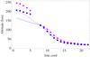 |
Fig. 7 Formation height above the 500 nm continuum level as a function of the line-cord index. Magenta dots and curve: FeI 630.1 nm line; blue dots and curve: FeI 630.2 nm line. Full lines show the uncorrected results, the discontinuity of the slope at index 8 is an artifact due to measurement difficulties in the contrast inversion layer. Dots show the results corrected for the inversion layer discontinuity, as explained in the text. |
Radiation temperature stratification derived from images in the FeI 630.15 nm line.
Radiation temperature stratification derived from images in the FeI 630.25 nm line.
3.4. Comparison with semi-empirical models
We can now compare our results with previously published semi-empirical models of the solar photosphere. The most recent ones have been established in Fontenla et al. (2006). The density stratification of semi-empirical models result from an hydrostatic equilibrium equation accounting for large-scale motions, and turbulent motions through a turbulent pressure velocity parameter. In quiet-Sun models, this parameter is identified with the micro-turbulent velocity derived from the fitting of spectral line widths. As noticed in Fontenla et al. (2006), this rather arbitrary choice reflects the difficulty in obtaining diagnostics for the gas pressure scale-height from observational data. In Fontenla et al. (2006), data obtained at the Precision Solar Photometric Telescope (PSPT) have been used to improve the models at the photospheric layers. Three different kinds of regions have been considered according to their location with respect to the chromospheric network. Here we compare our results with those of the average cell interior, denoted by model C. First we compare, in Fig. 8, the temperature stratification from Model C with the results given in Tables 3 and 4, as a function of the 630 nm continuum optical depth derived from the Eddington-Barbier approximation (levels 1 to 3 of the FeI 630.15 nm line have not been included, because they are strongly affected by non-LTE effects). Our measurements and the semi-empirical model agree very well.
We now compare the same temperature measurements, but as functions of the geometrical height above the base of the photosphere. This comparison is shown in Fig. 9. In this figure we used the corrected line core formation heights, as explained above, and we did not take into account the measurements performed at levels 5 to 7, formed in the contrast inversion layer. Figure 9 shows that the temperature stratification with respect to the geometrical height is very different in Model C and in our measurements. This discrepancy is caused by a disagreement on the relation between the continuum optical depth scale and the geometrical scale, i.e., probably, by problems in the solution of the hydrostatic equilibrium equation, in 1D semi-empirical modeling.
The last two columns of Tables 3 and 4 provide us with an empirical determination of the variation of the 630 nm continuum optical depth with the altitude in the low photosphere. We used this relation to derive the height variations of the absorption coefficient in the continuum at 630 nm through the simple formula  (13)The cross-spectral method we used is a differential method to measure height-differences, it thus ensures quite a good accuracy on the measurement of the denominator, but the optical-depth scale is determined from the Eddington-Barbier approximation. This limits the accuracy of the measurement of kc, in particular close to the continuum formation layer, where the optical depth varies very slowly between successive line-cord levels (typically for z between 20 km and 30 km). However, we verified that both lines give quite consistent values for this absorption coefficient in the low photosphere, as shown in Fig. 10.
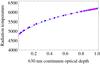 |
Fig. 8 Comparison of the radiation temperature variations of Model C (Fontenla et al. 2006) as a function of the 630 nm continuum optical depth (full line), with the radiation temperature measured in the FeI 630.1 nm line wings (magenta dots) and in the FeI 630.2 nm (blue dots). |
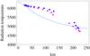 |
Fig. 9 Comparison of the radiation temperature depth variations of Model C of Fontenla et al. (2006) (full line) with the measured radiation temperature stratifications in the FeI 630.1 nm line (magenta dots) and in the FeI 630.2 nm (blue dots). The temperature stratification is not measured within the granulation contrast inversion layer between z = 130 km and z = 180 km. |
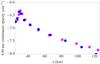 |
Fig. 10 Absorption coefficient of the low photosphere at λ = 630 nm on a log-scale as a function of the altitude in km. Results derived from the FeI 630.1 nm and the FeI 630.2 nm data are shown with magenta and blue dots, respectively. |
4. Discussion
We stress here that the radiation temperatures we measured in the low photosphere were determined from the average intensity observed at disk center at various line cords in the wings of the FeI 6315 nm and 630.25 nm lines. Averaging over the image corresponds to averaging over a roughly constant optical depth surface. In the same way, the formation heights of the images were measured from the perspective shift between images at successive line levels, that is, we measured the mean heights between surfaces at constant optical depths.
One of the main results of this paper is the measurement of the temperature gradient in the low photosphere, as shown in Figs. 8 and 9. The temperature gradient on the optical depth variable τ630 agrees with Model C; its value between τ630 = 1 and τ630 = 0.5, ∂log (T)/∂log (τ630) ≃ 0.11, is significantly lower than the theoretical value 0.25 for a gray atmosphere in radiative equilibrium.
For the temperature gradient on the geometrical height scale, we obtained slightly different values from the measurements performed independently in the FeI 630.15 nm and 630.25 nm line wings. On average we found that between z = 20 km and z = 120 km the radiation temperature of the photosphere decreases almost linearly from 6200 K to 5825 ± 65 K, the depth-gradient is thus –3.75 ± 0.65 K/km. This is significantly lower than the temperature-height gradient of Model C in the low photosphere. This seems to be an intrinsic problem arising in 1D radiative transfer modeling intended to fit average spectra formed in an inhomogeneous atmosphere. We quote here Uitenbroek & Criscuoli (2011): “The interpretation of an average spectrum from a horizontally inhomogeneous atmosphere in terms of a one-dimensional model will lead to an overestimate of the average temperature gradient in the atmosphere”. We also suspect that some of the assumptions used for solving the hydrostatic equilibrium equation in 1D semi-empirical models are probably not valid, such as those regarding the turbulent pressure parameter.
One might also imagine that a magnetic pressure term, due to weak ubiquitous turbulent magnetic fields in the quiet-Sun photosphere, such as those detected by their Hanle effect, could play a non-negligible role. In this respect, it is interesting to compare the order of magnitude of the turbulent pressure term of Model C,  , with turbulent velocities vturb on the order of 1.5 km s-1, and ρ on the order 2 × 10⁻⁷ g cm-3, with the magnetic pressure created by weak turbulent magnetic fields, with a quadratic mean strength on the order of 130 Gauss, as measured by Shchukina & Trujillo Bueno (2012). The two pressure terms are almost equal. The introduction of a magnetic pressure term, independent of density and temperature, with a negative height- gradient as measured by Milić & Faurobert (2012), in the pseudohydrostatic equilibrium of the solar photosphere would allow one to maintain the hydrostatic equilibrium while decreasing the density and gas pressure gradient in the photosphere.
Another significant result of this paper is the measurement of the height of the granulation contrast inversion layer, which is observed in the images at levels 8 to 5 in the FeI lines at 630 nm. We found that the base of this layer is located around 130 km
above the continuum formation level at 500 nm. This agrees well with the 3D numerical simulations of Cheung et al. (2007).
Acknowledgments
Hinode is a Japanese mission developed and launched by ISAS/JAXA, collaborating with NAOJ as a domestic partner, NASA and STFC (UK) as international partners. Scientific operation of the Hinode mission is conducted by the Hinode science team organized at ISAS/JAXA. This team mainly consists of scientists from institutes in the partner countries. Support for the post-launch operation is provided by JAXA and NAOJ (Japan), STFC (U.K.), NASA, ESA, and NSC (Norway).
References
- Cheung, M. C. M., Schüssler, M., & Moreno-Insertis, F. 2007, A&A, 461, 1163 [NASA ADS] [CrossRef] [EDP Sciences] [Google Scholar]
- Faurobert, M., Aime, C., Périni, C., et al. 2009, A&A, 507, L29 [NASA ADS] [CrossRef] [EDP Sciences] [Google Scholar]
- Faurobert, M., Ricort, G., & Aime, C. 2012, A&A, 548, A80 [NASA ADS] [CrossRef] [EDP Sciences] [Google Scholar]
- Fontenla, J., White, O. R., Fox, P. A., Avrett, E. H., & Kurucz, R. L. 1999, ApJ, 518, 480 [NASA ADS] [CrossRef] [Google Scholar]
- Fontenla, J. M., Avrett, E., Thuillier, G., & Harder, J. 2006, ApJ, 639, 441 [NASA ADS] [CrossRef] [Google Scholar]
- Grec, C., Aime, C., Faurobert, M., Ricort, G., & Paletou, F. 2007, A&A, 463, 1125 [NASA ADS] [CrossRef] [EDP Sciences] [Google Scholar]
- Grec, C., Uitenbroek, H., Faurobert, M., & Aime, C. 2010, A&A, 514, A91 [NASA ADS] [CrossRef] [EDP Sciences] [Google Scholar]
- Maltby, P., Avrett, E. H., Carlsson, M., et al. 1986, ApJ, 306, 284 [Google Scholar]
- Milić, I., & Faurobert, M. 2012, A&A, 547, A38 [NASA ADS] [CrossRef] [EDP Sciences] [Google Scholar]
- Neckel, H. 2003, Sol. Phys., 212, 239 [NASA ADS] [CrossRef] [Google Scholar]
- Neckel, H. 2005, Sol. Phys., 229, 13 [NASA ADS] [CrossRef] [Google Scholar]
- Orozco Suárez, D., Bellot Rubio, L. R., & Del Toro Iniesta, J. C. 2010, A&A, 518, A3 [NASA ADS] [CrossRef] [EDP Sciences] [Google Scholar]
- Shchukina, N., & Trujillo Bueno, J. 2012 [arXiv:1212.3048] [Google Scholar]
- Uitenbroek, H., & Criscuoli, S. 2011, ApJ, 736, 69 [NASA ADS] [CrossRef] [Google Scholar]
All Tables
Comparison of the line-cord opacity factors (1 + rφ(δλ)) derived from a Milne-Eddington model (ME) and from the Eddington-Barbier approximation (EB) for the FeI 630.15 nm line.
Radiation temperature stratification derived from images in the FeI 630.15 nm line.
Radiation temperature stratification derived from images in the FeI 630.25 nm line.
All Figures
|
Fig. 1 Center-to-limb variations of the mean intensity of the photosphere at 25 line-levels, normalized to the mean intensity of the continuum at disk center. Upper panel: FeI 630.1 nm line; lower panel: FeI 630.2 nm. The right sides of the figures show the measurements performed in the northern hemisphere as functions of 1 − cosθ (0 at disk center), the left sides show the results for the southern hemisphere as funtions of − (1 − cosθ). From the lower curve to the top one the line-cord index varies from 1 to 25 (line center to continuum level). Parabolic fittings (in red) are superimposed to the observed curves at line cords 1 to 9 and 20. The thin smooth line shows the fifth-order polynomial fitting of the continuum mean intensity, as given by Neckel (2005). |
| In the text | |
|
Fig. 2 Slope of the mean intensity CLV in the FeI 630.15 nm (left panel) and in the FeI 630.25 nm (right panel) measured at disk center for the 25 line cords, and normalized to 1 at level 25. Values fitting the northern and southern hemisphere measurements are shown in red and in blue, respectively. |
| In the text | |
|
Fig. 3 Parameters a and b of the parabolic fits of the mean intensity CLV as functions of the line-cord index. Upper panels: a and b parameters for the FeI 630.1 nm line; lower panels: a and b parameters for the FeI 630.2 nm line. Values measured in the northern and in the southern hemispheres are shown in red and blue, respectively. |
| In the text | |
|
Fig. 4 Phase (in radian) of the cross-spectrum of images at successive levels in the FeI 630.1 nm, measured at μ = 0.776 as a function of the spatial frequency given in pixel units. The frequency zero is at pixel 65. Upper row, from left to right: cross-spectra of images at levels 1 and 2, 2 and 3, and 3 and 4. Middle row, from left to right: cross-spectra of images at levels 4 and 5, 5 and 6, 6 and 7 (note the effect of contrast inversion), lower row, from left to right: cross-spectra of images at levels 11 and 12, 12 and 13, 13 and 14. |
| In the text | |
|
Fig. 5 Phase of the cross-spectrum of an image observed in the continuum and a numerically displaced image with a contrast inversion at high spatial frequencies. The red linear curve shows the phase corresponding to the imposed displacement of 0.05 pixel. The spatial frequency zero is at pixel 129. The cyan, blue, and magenta lines show how the measured slope would vary according to the width of the linear fitting interval at the origin, namely ±5 pixels, ±15 pixels and ±25 pixels, respectively. |
| In the text | |
|
Fig. 6 Perspective shifts measured between the continuum and images at four line levels as function of 1 − μ in the northern hemisphere, and − (1 − μ) in the southern hemisphere. Upper panel: results for the Fe1 630.1 nm line. Lower panel: results for the Fe2 630.2 nm. Red dots: line centers (level 1), light -blue dots: level 5, orange dots: line level 10, deep-blue dots: level 15. |
| In the text | |
|
Fig. 7 Formation height above the 500 nm continuum level as a function of the line-cord index. Magenta dots and curve: FeI 630.1 nm line; blue dots and curve: FeI 630.2 nm line. Full lines show the uncorrected results, the discontinuity of the slope at index 8 is an artifact due to measurement difficulties in the contrast inversion layer. Dots show the results corrected for the inversion layer discontinuity, as explained in the text. |
| In the text | |
|
Fig. 8 Comparison of the radiation temperature variations of Model C (Fontenla et al. 2006) as a function of the 630 nm continuum optical depth (full line), with the radiation temperature measured in the FeI 630.1 nm line wings (magenta dots) and in the FeI 630.2 nm (blue dots). |
| In the text | |
|
Fig. 9 Comparison of the radiation temperature depth variations of Model C of Fontenla et al. (2006) (full line) with the measured radiation temperature stratifications in the FeI 630.1 nm line (magenta dots) and in the FeI 630.2 nm (blue dots). The temperature stratification is not measured within the granulation contrast inversion layer between z = 130 km and z = 180 km. |
| In the text | |
|
Fig. 10 Absorption coefficient of the low photosphere at λ = 630 nm on a log-scale as a function of the altitude in km. Results derived from the FeI 630.1 nm and the FeI 630.2 nm data are shown with magenta and blue dots, respectively. |
| In the text | |
Current usage metrics show cumulative count of Article Views (full-text article views including HTML views, PDF and ePub downloads, according to the available data) and Abstracts Views on Vision4Press platform.
Data correspond to usage on the plateform after 2015. The current usage metrics is available 48-96 hours after online publication and is updated daily on week days.
Initial download of the metrics may take a while.