| Issue |
A&A
Volume 551, March 2013
|
|
|---|---|---|
| Article Number | A91 | |
| Number of page(s) | 26 | |
| Section | Astronomical instrumentation | |
| DOI | https://doi.org/10.1051/0004-6361/201220257 | |
| Published online | 28 February 2013 | |
Understanding synthesis imaging dynamic range
CSIRO – Astronomy and Space Science, PO Box 76, Epping, NSW 1710, Australia
e-mail: robert.braun@csiro.au
Received: 19 August 2012
Accepted: 19 January 2013
We develop a general framework for quantifying the many different contributions to the noise budget of an image made with an array of dishes or aperture array stations. Each noise contribution to the visibility data is associated with a relevant correlation timescale and frequency bandwidth so that the net impact on a complete observation can be assessed when a particular effect is not captured in the instrumental calibration. All quantities are parameterised as function of observing frequency and the visibility baseline length. We apply the resulting noise budget analysis to a wide range of existing and planned telescope systems that will operate between about 100 MHz and 5 GHz to ascertain the magnitude of the calibration challenges that they must overcome to achieve thermal noise limited performance. We conclude that calibration challenges are increased in several respects by small dimensions of the dishes or aperture array stations. It will be more challenging to achieve thermal noise limited performance using 15 m class dishes rather than the 25 m dishes of current arrays. Some of the performance risks are mitigated by the deployment of phased array feeds and more with the choice of an (alt,az,pol) mount, although a larger dish diameter offers the best prospects for risk mitigation. Many improvements to imaging performance can be anticipated at the expense of greater complexity in calibration algorithms. However, a fundamental limitation is ultimately imposed by an insufficient number of data constraints relative to calibration variables. The upcoming aperture array systems will be operating in a regime that has never previously been addressed, where a wide range of effects are expected to exceed the thermal noise by two to three orders of magnitude. Achieving routine thermal noise limited imaging performance with these systems presents an extreme challenge. The magnitude of that challenge is inversely related to the aperture array station diameter.
Key words: instrumentation: interferometers / methods: observational / techniques: interferometric / telescopes
© ESO, 2013
1. Introduction
Dynamic range limitations in synthesis imaging arise from three distinct categories of circumstance: 1. instrumental artefacts; 2. imaging artefacts; 3. incomplete calibration of the instrumental response. The first category can be addressed by insuring a linear system response to signal levels together with other design measures within the receiver and correlator systems that minimise spurious responses. While challenging to achieve, the engineering requirements in this realm are moderately well defined and this class of circumstance will not be considered further in the current discussion. Some of the specific relevant effects, such as “closure errors” and quantisation corrections are discussed in Perley (1999). The second category includes a range of effects, from the well understood smearing effects that result from a finite time and frequency sampling to the imaging challenges associated with non-coplanar baselines as discussed in Cornwell et al. (2008). The third category is one that is less well understood and documented. Several important effects in this area are also discussed by Perley (1999); including imperfect polarisation calibration, inadequate (u,v) coverage, and numerical modelling errors. In this study we will attempt to identify and quantify the phenomena that influence synthesis image dynamic range more generally.
The approach we adopt is the consideration of a wide range of calibration issues that influence interferometeric imaging. For each of these effects we develop a parameterised model that quantifies the fluctuation level due to that effect on the measured visibilities, together with its correlation timescale and frequency bandwidth. We then assess the equivalent image noise due to each effect. While some effects contribute directly to the image noise, many contribute to image noise in an indirect manner via the self-calibration process. We demonstrate that both direct (in-field) and indirect (out-of-field) noise contributions typically have a comparable image magnitude if it has proven necessary to employ self-calibration. By tracking each calibration effect individually, it becomes possible to quantify how each contributes to a final image noise level. The purpose of calibration and imaging strategies is to accurately model all of the effects that might limit imaging performance. We do not attempt to evaluate how well any specific algorithm or strategy performs in this regard. We only provide an indication of the precision with which each of these calibration effects must be addressed for an assumed telescope performance specification, so as not to form an ultimate limitation on performance.
2. Calibration errors
A key factor that determines image dynamic range is calibration of the instrumental gain. Instrumental gain, in this context, should be considered to be the (spatial, polarisation, frequency) response in (amplitude, phase) as function of time of each of the antennas (be they aperture array stations, or the phased-array fed- or single pixel fed-dish beams) of a synthesis array. Traditional array calibration methods, employing semi-continuous (minute scale) noise source injection and occasional (hour scale) observations of well-characterised calibration sources routinely achieve a calibration precision at GHz frequencies of a few percent in amplitude and about 10 degrees of phase. This gain calibration precision, φC = 0.2, is only sufficient to achieve an image dynamic range of less than about 1000:1 in full track observations with existing arrays. A rough estimate of the relation between these quantities is derived by Perley (1999). The dynamic range, D, is about,  (1)for MT independent time and MF frequency intervals and N antennas that each have independent gain errors of magnitude φ. What constitutes an independent time sample depends critically on the nature of the gain error together with both baseline length and field of view; varying from hours to fractions of a second. Similar considerations also apply to what constitutes an independent frequency interval. Improvements of the image dynamic range from this base level rely on self-calibration. Self-calibration (e.g. Cornwell & Fomalont 1999) consists of the iterative modelling of the sky brightness distribution together with the instrumental calibration. Self-calibration only works when two conditions are met:
-
1.
there are a sufficiently small number of degrees of freedom inthis model relative to the number of independent data constraints;
-
2.
the signal-to-noise ratio in the data for each antenna is sufficiently high within each solution interval.
The number of data constraints (for a given frequency channel and polarisation state) is ND ≈ N2/2 over the solution timescale over which all model parameters are constant. Significant instrumental/ atmospheric/ ionospheric gain fluctuations typically occur on (sub-) minute timescales. If the sky brightness is dominated by a single compact source, then the number of degrees of freedom, NF, is NF ≈ 1 + N, and its clear that the system is highly over-determined (ND ≫ NF) for the solution of the N antenna gains in a single source direction within each solution interval. If, on the other hand, the sky brightness is characterised by a large number of widely separated components, NC, each of which is represented by multiple variables (e.g. a peak brightness, two positions, two sizes and an orientation) that approaches N2 in number, then its clear that difficulties can arise. In that case, it has become customary to assume that the spatial instrumental response to the sky brightness remains time invariant, so that the total number of degrees of freedom, NF ≈ 6NC + MTN still remains small relative to the complete observation that comprises NT = MTN2/2 total independent data constraints. We will explore below the circumstances under which this assumption breaks down. In practise, the number of degrees of freedom will be closely tied to the specific calibration algorithm that is employed. There are clearly great benefits to minimising NF with an algorithm that is optimally matched to the problem.
The requirement of sufficient signal-to-noise in the data from each antenna has a direct bearing on the precision of the self-calibration solution that can be achieved. Cornwell & Fomalont (1999) give an estimate for the residual calibration error for a given solution timescale, τS, as φ(τS) = σ(τS)/ [(N − 3)0.5S] in terms of the fluctuation level of a single visibility σ(τS) and a single dominant, unresolved source of flux density, S. In the case of a more complicated sky brightness distribution composed of NC widely separated discrete components of total flux density STot, this becomes: ![\begin{equation} \phi(\tau_{\rm S}) = \sigma(\tau_{\rm S})N_{\rm C}^{0.5}/\left[(N-3)^{0.5}S_{\rm Tot}\right] , \label{eqn:phi} \end{equation}](/articles/aa/full_html/2013/03/aa20257-12/aa20257-12-eq23.png) (2)since the NC components will not contribute coherently to the net visibility vector. A practical solution timescale in the single, on-axis source case would be tied to the intrinsic fluctuation timescale of about a minute, while for the multiple component case, it will be determined by the off-axis distance on the sky of these components. As we will see below, this will be comparable to a single integration time; typically one to ten seconds, for sources within the main beam of the antenna. When both these conditions are satisfied to a sufficient degree, it has proven possible to achieve image dynamic range, D = SMax/σMap, defined to be ratio of peak brightness, SMax, to the image root mean square (RMS) fluctuation level, σMap, of more than one million to one with current arrays after considerable effort by “black belt” level interferometrists. Its vital to note that the highest dynamic range imaging that has been achieved to date (e.g. Smirnov 2011b) is associated with fields dominated by particularly bright, yet simple sources. Fields that are dominated by more typical complex sources have not achieved anything comparable.
(2)since the NC components will not contribute coherently to the net visibility vector. A practical solution timescale in the single, on-axis source case would be tied to the intrinsic fluctuation timescale of about a minute, while for the multiple component case, it will be determined by the off-axis distance on the sky of these components. As we will see below, this will be comparable to a single integration time; typically one to ten seconds, for sources within the main beam of the antenna. When both these conditions are satisfied to a sufficient degree, it has proven possible to achieve image dynamic range, D = SMax/σMap, defined to be ratio of peak brightness, SMax, to the image root mean square (RMS) fluctuation level, σMap, of more than one million to one with current arrays after considerable effort by “black belt” level interferometrists. Its vital to note that the highest dynamic range imaging that has been achieved to date (e.g. Smirnov 2011b) is associated with fields dominated by particularly bright, yet simple sources. Fields that are dominated by more typical complex sources have not achieved anything comparable.
Rather than specifying some arbitrarily high numerical value of the dynamic range as a goal for a particular instrument or design, a more useful requirement might be that the instrument routinely achieves thermal noise limited performance even after long integrations. Since the noise in a naturally weighted synthesis image is simply related to the visibility noise as, ![\begin{equation} \sigma_{\rm Map} = \sigma(\tau_{\rm S})/[M_{\rm T} M_{\rm F} N (N-1)/2]^{0.5}, \label{eqn:sens} \end{equation}](/articles/aa/full_html/2013/03/aa20257-12/aa20257-12-eq27.png) (3)we can assess individual contributions, denoted by subscript i, to the final image noise by considering their magnitude on a self-cal solution timescale, σi(τS), together with the values of MTi and MFi which apply to each particular contribution. It is important to stress that the equivalent image noise calculated in Eq. (3) will only represent an actual image noise when it relates to objects within the image field of view. For effects that pertain to sources beyond the field of view the influence is more indirect as will be discussed in detail below. However, when self-calibration is employed, even the out-of-field error contributions will result in this magnitude of image fluctuation due to their adverse impact on the self-calibration error. Equation (3) will be used to track the magnitude of the different contributions to self-calibration error while taking into account the very different correlation timescales and bandwidths that apply to each.
(3)we can assess individual contributions, denoted by subscript i, to the final image noise by considering their magnitude on a self-cal solution timescale, σi(τS), together with the values of MTi and MFi which apply to each particular contribution. It is important to stress that the equivalent image noise calculated in Eq. (3) will only represent an actual image noise when it relates to objects within the image field of view. For effects that pertain to sources beyond the field of view the influence is more indirect as will be discussed in detail below. However, when self-calibration is employed, even the out-of-field error contributions will result in this magnitude of image fluctuation due to their adverse impact on the self-calibration error. Equation (3) will be used to track the magnitude of the different contributions to self-calibration error while taking into account the very different correlation timescales and bandwidths that apply to each.
As noted above, a major simplifying assumption that is often implicitly, if not explicitly, invoked is that of a time-invariant observed “sky” during the period of data acquisition. The underlying assumption is that neither the radio sky nor the (spatial, polarisation, frequency) components of the instrumental response vary with time and that only a single (amplitude, phase) term is sufficient to capture the time variable nature of the instrumental response. What if this is not the case?
2.1. Far sidelobes
The assumption of a stationary sky brightness will break down in practise for several reasons. Firstly, there is the residual all-sky response due to the far sidelobe pattern of the antenna. The far sidelobe attenuation of an antenna relative to the on-axis response, ϵF, is given approximately by the ratio of the effective area of a single dipole to that of the entire antenna,  (4)with a proprotionality constant ηF that is tied to the quality of aperture illumination and varies between about 0.1 < ηF < 1 in practise. The (λ/d)2 dependence is a manifestation of physical optics and applies to both blocked and unblocked apertures. Far sidelobe levels have been accurately determined for the 25 m diameter Very Long Baseline Array (VLBA) antennas at 1717 MHz by Dhawan (2002). Peak sidelobe levels of about –53 dB were measured at 30–110 degrees off-axis, yielding ηF ≈ 0.1. Dhawan (2002) note that while these VLBA levels are in good agreement with theoretical expectations, the values for Very Large Array (VLA) antennas were about 6 dB higher at that time (ηF ≈ 0.4), likely due to non-optimum illumination by the 20 cm feed lens system that has since been replaced in the Jansky Very Large Array (JVLA) upgrade. The prime focus fed 25 m diameter dishes of the Westerbork Synthesis Radio Telescope (WSRT) have measured far sidelobe levels at λ = 49 and 92 cm that are consistent with ηF ≈ 0.1 (Braun 1993). All radio sources above the horizon are attenuated by only this factor when they appear in a far sidelobe peak of the antenna. As the mainbeam of the antenna is used to track a source on the sky, the apparent brightness of the sky will vary due to the rising and setting of specific sources relative to the antenna horizon, but also due to changes in the far sidelobe response including, but not limited to, rotation of that pattern relative to the sky for an antenna mount that does not compensate for parallactic angle. The far sidelobe voltage response pattern of an antenna consists of local maxima and minima that are comparable to the main beam in size and separated by nulls. The basic pattern will have a radial frequency scaling, but may also contain additional frequency dependence, for example when multi-path propagation conditions are present.
The properties and density of radio sources are summarised in Table 1. Values are based on the NRAO VLA Sky Survey (NVSS; Condon et al. 1998) for source densities and median flux densities in each bin at GHz frequencies, and Windhorst (2003) for the median angular size and spectral index. Some care needs to be exercised with the interpretation of the angular size, since in many cases this refers to the separation of more compact components, rather than to the effective diameter of a diffuse source. This is particularly true for the brightest GHz source counts that are dominated by luminous classical double sources down to about 30 mJy. Below about 30 mJy, the source counts begin to be dominated by lower luminosity, edge-darkened radio galaxies and below about 0.1 mJy by star forming galaxies (e.g. Wilman et al. 2008).
Statistical source properties of the extragalactic sky at 1.4 GHz in bins of 0.5 dex.
A good indication for how the flux density of high luminosity radio galaxies varies with scale is given in Fig. 1 showing the power spectrum of Cygnus A based on a VLA A+B+C+D configuration 6 cm image of Perley et al. (1984). The solid line is the average normalised power as function of inverse scale, deconvolved for PSF tapering in the observation based on the short-dashed curve. The long-dashed curve is a power law of slope –0.75 which provides a reasonable representation of the trend for scales up to 30 times smaller than the source size. For statistical purposes, the Cygnus A power spectrum can be represented by the sum of four Gaussian components as shown by the dotted curve that has relative angular scales of (1:0.29:0.039:0.0067) and amplitudes of (0.648:0.237:0.107:0.008). Such a representation is clearly inadequate for detailed modelling of individual sources. From the combination of number densities and source sizes in Table 1 together with the power spectrum in Fig. 1, one can construct a composite fluctuation spectrum due to the high luminosity extragalactic background sources within 2π steradians. This is shown in Fig. 2 as the solid line, while the short-dashed curves are the contributions from the individual flux bins down to 30 mJy from Table 1. Within each flux bin, we form the incoherent sum of the relevant sources by taking the square root of the source number multiplied by the median flux of that bin. Similarly, the composite fluctuation level is taken to be the square root of the sum of the squares of the bin contributions. This is intended to describe the net composite fluctuation level in an interferometric visibility for a given baseline length. The net composite fluctuation level is well fit by a power law of slope –0.85 in baseline length from a base level of 450 Jy at 1 km as shown by the long-dashed curve.
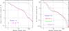 |
Fig. 1 Relative visibility amplitude of Cygnus A (left) and the Sun (right) are shown as the solid curves. The short-dashed curve shows the point spread function of the observations, while the long-dashed curve a power-law approximation. The dotted curve is a sum of four (left) and three (right) Gaussians that approximates the measured spectra. Both the active (1999APR11) and quiet (1993NOV06) Sun are shown. |
The other important parameter to quantify is the effective number of model components that would be needed to represent the sky brightness distribution. Within each flux bin of Table 1 we have taken the number of sources within 2π steradians and scale this with the inverse of the normalised power spectrum shown in Fig. 1. In this way, as each source becomes resolved it is distributed into a proportionally larger number of fainter components. We then form the weighted sum of components over flux bins using a weighting factor equal to the median flux of that bin. The total effective component number is shown as the solid line in Fig. 2, while the individual bin contributions are plotted as the short-dashed lines. As expected, only a few hundred components dominate the sky on all baselines between about 0.5 and 50 km. On longer baselines the total number increases approximately as a power law of baseline with slope ~0.4 from a base level of 100 on 1 km baselines as shown with the long-dashed curve.
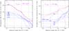 |
Fig. 2 Incoherent visibility “noise” due to 2π steradians of the extragalactic sky (left) and the corresponding number of flux-weighted components (right) as function of baseline length (angular scale). Visibility “noise” is completely dominated by the brightest source bin out to baselines of about 30 km that would require several hundred components to adequately model. |
With the –50 dB peak far sidelobe level of a 25 m dish observing at 25 cm, one hemisphere of the extragalactic radio sky would contribute some 5 mJy of noise-like fluctuations to visibility measurements on 1 km baselines. Adequate modelling of these sources would require about 100 components on this same scale. On 10 km scales such fluctuations will have declined to the 0.7 mJy level and would require some 100’s of components to model.
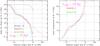 |
Fig. 3 Visibility “noise” due to the active and quiet Sun (left) and the corresponding number of components (right) as function of baseline length (angular scale). |
The Sun is the other major contributor to residual visibility fluctuations when not adequately modelled. We plot the relative visibility amplitude of the Sun in Fig. 1, based on 6 cm VLA mosaic images kindly provided by (White 2002, and priv. comm.). The two observing dates correspond to relatively active and quiet portions of the solar cycle. The solar power spectrum can be well modelled by the sum of three Gaussian components, as shown by the dotted curve, that have relative angular scales of (1:0.0625:0.0156) and amplitudes of (0.9645:0.0302:0.0053). The corresponding visibility “noise” and component number are plotted in Fig. 3 as function of baseline length. The visibility modulation level was taken to be the power spectrum of Fig. 1 divided by the square root of component number to account for the fact that the individual solar flux components will not sum coherently. The 1.4 GHz integral flux on these dates has been scaled to an assumed total of 100 sfu on 99APR11 and 50 sfu on 93NOV06 in line with the daily solar monitoring data from those epochs. With 50 dB of attenuation, there is still a residual fluctuation level of about 10 mJy on 1 km scales that would require about 100 components for adequate modelling.
2.1.1. Radio frequency interference
Another contribution to the far sidelobe response from the telescope environment is that of radio frequency interference (RFI) from ground-based, aerial and space-based sources. Clearly, the greater the degree of attenuation outside of the main beam, the more straightforward it becomes to deal with the power levels of non-astronomical transmissions. In view of the great diversity of RFI attributes, we will not attempt to characterise them here. We simply note that adequate RFI recognition, excision or mitigation will be essential to achieving thermal noise limited performance. There are many potential telescope locations and frequency bands in which RFI will preclude high performance imaging.
2.1.2. The ionosphere and atmosphere
A significant complicating factor in wide-field imaging is the direction dependent nature of propagation effects relative to a ground-based telescope array. The diffractive and refractive effects of the ionosphere and troposphere (Intema et al. 2009; Smirnov 2011a) make it necessary to determine distinct calibration solutions for sources separated by more than about 1 degree and timescales of about 1 min. The situation is further complicated for an array that is spatially extended relative to the physical size of density fluctuations, since the array is in the near-field of these fluctuations so that different telescopes have distinct propagation paths through the medium and a distant thin screen approximation is no longer valid. The relevant size scale for traveling ionospheric disturbances (TIDs) is a few km. While we will not attempt to quantify the impact of residual solution errors, we note the necessity for distinct, time and position dependent calibration solutions due to these effects.
2.1.3. The role of a global sky model
One might consider that a major aid to the self-calibration problem would be the provision of a high quality model of the entire radio sky at each frequency of an observation. To the extent that intrinsic source variability or propagation effects (in the interstellar, interplanetary, ionospheric or tropospheric media) were negligible this might eliminate many degrees of freedom in the sky model. While undoubtedly of great benefit, a global sky model will only partially reduce the number of degrees of freedom in the model (source positions), since a remaining unknown is generally the instrumental response in the direction of each source at each solution time. The accuracy with which far sidelobe responses of an antenna system can be predicted at any specific location is, conservatively, no better than a factor of two, implying that this prediction has little value in constraining a solution for the apparent brightness of each source within an observation. Although very significant effort is being expended to improve the prediction of far sidelobe responses in the aperture array domain (Wijnholds et al. 2010) it is not yet clear how effective these will be in practise. Far sidelobe responses are influenced by the surface irregularities of dishes, or equivalently, the gain and radiation pattern variations of individual aperture array elements. As such they will be different for each dish or station of an array and are likely to be time variable due to many environmental effects, including gravitational distortions and temperature gradients.
In the event that the global sky model also incorporates an extremely high fidelity, high resolution representation of every relatively bright source in the sky, it would provide an invaluable resource for accurate self-calibration. As will become apparent subsequently, the accurate modelling of the random sources that happen to occur within the field of view is often the primary limitation to the dynamic range that can be achieved. While this has been put forward as the preferred calibration method for survey projects such as planned with the LOw-Frequency Array for Radio astronomy (LOFAR; e.g. Heald et al. 2010) in practise it is likely to be the ultimate outcome of a multi-year data acquisition and source modelling effort, rather than a convenient starting point for a random field of interest.
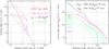 |
Fig. 4 Measured visibility “noise” due to the NVSS > 10 Jy sky as seen by the VLA C configuration without primary beam attenuation (left). The two solid curves show the fluctuation level with and without the inclusion of the Sun. The two dashed curves include the effects of time and frequency smearing and are overlaid with representative power-law approximations. Visibility “noise” per solid angle due to the NVSS sky (right). The rms contribution of NVSS sources, normalised to a one square degree field of view, is plotted as function of baseline length. Flux bins from Table 1 are shown individually with the labelled curves. The root squared sum of contributions of the bins <10 Jy is shown as the solid line, together with an overlaid powerlaw fit. |
2.1.4. Time and bandwidth smearing/correlation
The visibility response to distant off-axis sources will be modified by several effects, most notably time- and bandwidth- smearing for the finite integration times and frequency resolution used in an observation. This can be viewed both positively and negatively. The peak visibility response will be diminished by these smearing effects and this will be beneficial in reducing noise-like modulations. However, if the source is still bright enough that it must be modelled, then the smearing will adversely impact the quality of that modelling and contribute to residual gain errors in the calibration. The angular extent of time smearing of the response due to Earth rotation is given approximately by,  (5)for an angular rotation rate ω, (15 deg/h) an integration time, τS, and an offset angle from the phase centre, θ. For a source on the celestial pole viewed by an east-west baseline, this smearing is along a circular track, while for other circumstances the smearing direction is more complex. The bandwidth smearing has an extent,
 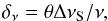 (6)for a fractional bandwidth ΔνS/ν and is in a radial direction. For example, an unresolved source that is offset from the pointing direction by 1 radian that is sampled with an integration time of 1 s with a fractional bandwidth of 10-4 will suffer about 15 arcsec of both time smearing and bandwidth smearing. The specific choice of integration times and averaging bandwidths is determined by the need to keep these effects at the level of a small fraction, ηS, of the synthesised beamwidth within the antenna main beam. In terms of a dish/station diameter, d, and array of baseline, BMax, this implies an integration time no longer than,
  (7)and a fractional bandwidth no larger than,
  (8)For example, for ηS = 0.1,d = 25 m and BMax = 25 km, the requirements are Δν⋆/ν ≤ 10-4 and τ⋆ ≤ 1 s. Exactly the same considerations can be used to evaluate the likely time and frequency intervals over which particular types of calibration errors might be correlated. If the calibration error relates to a source that is near the half power point of the main beam, this corresponds to δτ = δν = λ/B and θ = λ/(2d) in Eqs. (5) and (6), which will be correlated over time intervals of,
  (9)and bandwidths,
  (10)For example, for d = 25 m and BMax = 25 km, the calibration errors associated with sources near the half power point of the main will be correlated over Δν/ν ≈ 2 × 10⁻³ and τ ≈ 28 s. In the far sidelobe regime, with θ = 1 radian, the correlation time reduces to,
  (11)and bandwidth to,
  (12)
(12)
2.1.5. Visibility consequence
The consequence of unmodelled off-axis sources in the visibility data is a modulation of the visibilities with a magnitude equal to that of the unmodelled source. Unresolved and unsmeared sources will have the same modulation amplitude on all observed baselines, while resolved and/or smeared sources will have a modulation amplitude that decreases with increasing baseline length. Since these are periodic modulations, with a modulation wavelength, m = λ/θ, that is very short for large pointing offsets, they will partially cancel when averaged over finite time intervals or within gridded visibility cells. However, the presence of such residual modulations will negatively influence the quality of the self-calibration that can be achieved, particularly on relatively short timescales over which the cancellation will be increasingly imperfect. In the case where successive integration times sample visibilities that are offset from one another by a significant fraction of λ/θ, i.e. baselines of length greater than, B > λBMax/(ηSθd), or about a km for GHz observations with θ = 1 radian, such unmodelled sources will add a noise-like contribution in quadrature to the visibility noise σ(τ) and directly impact the calibration precision φ, and ultimately the final image noise level.
We have attempted to verify the analytic estimates of far sidelobe effects by simulating model visibilities as observed by the VLA C configuration at 1.4 GHz. All radio sources within the NVSS database brighter than 10 Jy and above the local VLA horizon at LST 12:00:00 were added to an otherwise empty visibility file of 12 h duration using the miriad (Sault et al. 1995) task uvgen. Each catalogued source was assumed to be composed of the sum of four Gaussian contributions with angular sizes of (1:0.29:0.039:0.0067) relative to the tabulated full width at half maximum (FWHM) and amplitudes of (0.648:0.237:0.107:0.008) relative to the integrated flux density. The response was calculated relative to a pointing centre at (RA, Dec) = (12h,34deg) both with and without a three Gaussian component model of the Sun (assumed to be at (RA, Dec) = (9h, − 11deg) when present) as illustrated in Fig. 3. The intrinsic fluctuation levels are indicated by the solid curves in Fig. 4. The residual fluctuations including the smearing effects of a 10 s integration time and Δν/ν = 10-3 frequency sampling are indicated by the dashed curves. (We note that since the uvgen task does not provide explicit support for time and bandwidth smearing, these effects were introduced by generating a highly oversampled simulation that was vector averaged appropriately after calculation.) The intrinsic fluctation spectra are flatter by unit slope compared to those which include both smearing effects, as expected. No primary beam attenuation has been applied. Representative power law approximations of the post-smearing fluctuation levels are,  (13)for nighttime observing and,
 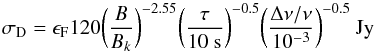 (14)with the Sun present. The ϵF term represents the far side-lobe response from Eq. (4). The extragalactic contribution scales roughly as ν-0.8, given the steep spectra of the brightest sources, while the solar spectrum at GHz frequencies is relatively flat. The baseline length is normalised with Bk = (ν/1.4 GHz)-1 km. These measured fluctuation spectra are quite similar to those obtained by the analytic estimate shown previously in Figs. 2 and 3 although with a slightly flatter slope when the individual source attributes and positions are employed rather than the tabulated binned source properties. Clearly, the daytime power-law approximation is only valid for baselines less than about B/Bk = 3, where the solar contribution dominates over that of the extragalactic sky.
An important aspect of the far sidelobe contribution to visibility “noise” is that it is essentially uncorrelated between adjacent frequency channels and time stamps. Equations (12) and (11) yield Δν/ν ≈ 10-4 and τ ≈ 1.5 s at a typical off-axis distance of 1 radian. While this noise contribution may adversely influence individual solutions, at least it will average down substantially during long tracks and over significant bandwidths. The relevant values of MTi and MFi are given simply by the total number of solution intervals in time and frequency, as,  (15)and
  (16)for a total observing time τT and bandwidth ΔνT.
2.1.6. Image consequence
The image plane consequence of unmodelled sources is influenced by some additional factors. Sources that lie beyond the edges of a synthesis image will be aliased back into that image. The degree of suppression of such aliased responses is determined by the convolving function that is used to grid the visibility data. This constitutes a degree of averaging of the highly modulated visibilities (as discussed above) to provide partial cancellation of off-axis responses. Gridding functions that are currently used in synthesis imaging provide about 40 dB suppression of the aliased response in the far sidelobe regime (e.g. Briggs et al. 1999). What the gridding function will not suppress is any synthesised beam sidelobes of distant sources that would naturally occur within the image. Since the apparent brightness of a far sidelobe source will often be highly time variable, it is the instantaneous synthesised beam quality which becomes important in this regard. In the most extreme case of a one dimensional array configuration, the instantaneous synthesised beam far sidelobes can have amplitudes of 100% so that unmodelled sources can add spurious structure to the image with very little suppression beyond that provided by the main beam. Even in the case of a regular three arm configuration such as used in the VLA, the instantaneous synthesised beam has peak sidelobe levels of 10’s of percent. What prevents this factor from becoming dominant in most broad-band continuum applications is the radial frequency scaling of the synthesised beam pattern, including its sidelobes. The sidelobe pattern will partially cancel in the frequency averaged response.
In addition to the “direct” image consequence of unmodelled far side-lobe sources discussed above, there is the “indirect” consequence of such sources. Within each self-cal solution interval, the noise-like visibility modulation of unmodelled sources will limit the precision of the self-cal solution as shown in Eq. (2). The net image plane noise due to degradation of the self-cal solution can be estimated from the visibility fluctuation level σ(τS), by combining Eqs. (1) and (2) giving, 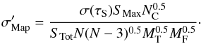 (17)The ratio of “indirect” to “direct” contributions (Eqs. (17) and (3)) is then,
 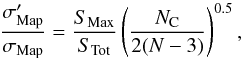 (18)which is approximately unity for arrays with N ≈ 30.
2.2. Near-in sidelobes
In addition to the issue of far-sidelobes, is that of the near-in sidelobe pattern of the antenna response. Any aperture blockage and non-zero illumination taper at the edges of the antenna will give rise to near-in sidelobes in the antenna response. For a uniform aperture illumination, such as might be employed for an aperture array station, these will have a peak value, ϵS = 0.1, while the more tapered, but “blocked” illumination patterns of prime focus and symmetric Cassegrain-fed dishes yield peak near-in sidelobes of about ϵS = 0.02. The unblocked 100 m Green Bank Telescope (GBT) aperture has near-in peak sidelobe levels of less than 1% at 1.4 GHz (Robishaw & Heiles 2009), although these have significant azimuthal modulation.
Near-in sidelobes complicate the calibration and imaging problem in a number of ways. Significant sidelobe responses will increase the region of sky that must be modelled with high precision to enable self-calibration. The increase in the number of degrees of freedom that are absorbed by sky components may then limit the precision of the self-cal solution as outlined above. Since these components are significantly further off-axis than main-beam components, they will also require proportionally shorter solution timescales to be employed, which impacts the solution precision via the visibility signal-to-noise constraint. This is particularly problematic if the sidelobe pattern is not fixed on the sky during source tracking, since one then encounters the under-determined self-cal solution condition more rapidly. Some deconvolution aspects of this problem have been addressed by Bhatnagar et al. (2008) with extensive modelling of both the VLA main beam and its near-in sidelobe and polarisation response, including its changing orientation relative to the sky. A self-cal implementation has been described in Bhatnagar et al. (2004). When it proves too challenging to model sources occuring within the near-in sidelobes they will yield a residual visibility modulation of, 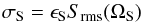 (19)in terms of the net rms source brightness, Srms, within the area of the sidelobe pattern, ΩS. The net visibility fluctation level due to the NVSS source population per unit area is shown in the right hand panel of Fig. 4. This plot is similar to Fig. 2 but is calculated for a reference solid angle of 1 deg2 rather than 2π sr, and the summation excludes the two brightest flux bins so that it better represents a random, but “quiet”, piece of the sky that does not include the 100 or so brightest sources per hemisphere. A power-law representation of the net visibility fluctuation level is given by,
 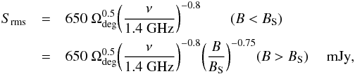 (20)where the rms brightness scales roughly as ν-0.8, and the baseline length is normalised to the break at about BS = 3(ν/1.4 GHz)-1 km, below which the rms flux saturates. Of note in Eq. (20) is the square root dependence on solid angle, which accounts for the incoherent vector summation of sources in the field of view. In cases where the main beam field of view exceeds about 200 deg2, the “quiet” sky approximation is clearly no longer relevant, and the complete source population must be considered yielding,
 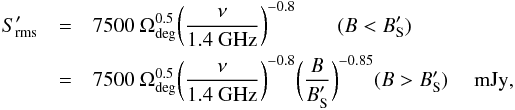 (21)with
 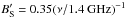 km. As will be seen below, the values of Srms and
  are intermediate between the peak brightness, SMax, and the integrated brightness, STot, within a field of size Ωdeg.
The telescope main beam has its first diffraction null at a radius of 1.22λ/d radians which is also approximately the main beam FWHM. This corresponds to a main beam solid angle, 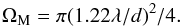 (22)The first diffraction sidelobe extends from radius (1.22λ/d − 2.44λ/d) and so has solid angle of,
  (23)The correlation timescale and bandwidth for these modulations due to sources offset from the pointing direction by θ = λ/d will be τ ≈ d/(ωB) and Δν/ν ≈ d/B, yielding,
  (24)and,
  (25)Near-in sidelobe patterns of dishes have been shown to have substantial frequency modulation at the 10% level (Popping & Braun 2008) with a periodicity of about fS ≈ c/2lC Hz, for a vertex to prime focus “cavity” separation, lC. For Cassegrain optics the relevant separation, lC, appears to be approximately that of the primary and subreflector, while for offset Gregorian designs it is that of the feed and subreflector. While such sidelobe modulation has only been demonstrated to date with frequency resolved holography on the WSRT dishes, this effect is intimately related to the “standing wave” phenomenon that afflicts all current dish designs. The correlation bandwidth will be about half a period, Δν ≈ c/(4lC) which yields,
  (26)The larger of the two values given by Eqs. (25) and (26) provides the better estimate of the independent sample number in the full observation.
2.3. Main-beam issues
There are several ways in which attributes of the main beam of the antenna will influence image dynamic range. In the case of aperture arrays, it is conceivable that the antenna main beam may be continuously changing as a field is tracked on the sky due to the changing geometric foreshortening of the aperture. In this case, the main beam sky brightness model will be highly time variable and one will need to operate essentially in the snap-shot self-cal mode, without the benefit of the factor of MT additional data constraints that come with a time-invariant main beam model. In the event that different aperture array main beams were to apply to different antennas (as implemented for the three variants of the LOFAR high band antennas) this is further complicated, since there are only smaller subsets of the visibilities (e.g. N2/8) for which the same snap-shot sky brightness model would apply, greatly diminishing the number of relevant data constraints relative to sky brightness components. A means of compensating for different main beam types as well as main beam variability has been termed the A-Projection method and is decribed by Bhatnagar et al. (2008). The method employs a gridding convolution function for the visibilities that compensates for modelled main beam properties. This provides an exact method for the “reverse” calculation of visibilities given a sky model, but only an approximate “forward” calculation of the dirty image from the acquired data. In cases where there are substantial differences between- or time variability in- the main beam properties of the visibilities, there will be a position dependent synthezied beam and signal-to-noise ratio which may limit the quality of deconvolution which can be achieved.
2.3.1. Pointing errors
A second important class of main beam influences relates to the antenna pointing accuracy (either mechanical for dishes or electronic for aperture arrays). Pointing variations will introduce a strongly time variable component to the radio sky brightness model for components that are significantly off-axis. If the sky brightness model is dominated by such widely distributed components, then pointing variations may again push one into the snap-shot self-cal mode. For the simplest form of pointing error, that preserves main-beam shape, the model variations could in principle be captured with only two additional degrees of freedom per antenna (the two perpendicular pointing offsets). Bhatnagar et al. (2008) have also considered this class of error in their study. Pointing errors that are a fraction, βP, of the main beam of size, P = βPλ/d radians, are most serious where they introduce the strongest absolute modulation in apparent source brightness. For a Gaussian approximation to the main beam, M = exp( − 0.5(θ/s)2), the maximum spatial derivative occurs at a bore-sight offset equal to the dispersion, s = λ/(2d), and has amplitude exp( − 0.5)/s rad-1, giving an amplitude modulation, ϵP = βPλ exp( − 0.5)/(sd) = 2βPexp( − 0.5) ≈ βP. The maximum amplitude modulation expected on the flanks of the main beam is thus comparable to the pointing error expressed as a fraction of the main beam size, ϵP ≈ βP. Actual main beam shapes can only be well-fit by a Gaussian out to about 10% of the peak response. Beyond this radius lies a deep response minimum followed by the near-in sidelobes. The main beam power pattern of an interferometer arises from the product of the complex voltage response patterns of each pair of antennas. The deep response minimum in the power pattern corresponds to the region where the sign of the voltage pattern of each antenna changes from positive to negative. A uniformly illuminated circular aperture has a voltage response pattern given by V(x) = 2J1(x)/x, where J1(x) is the Bessel function of the first kind of order 1. Evaluation of the radius at which the product of sky area (πx2) with V(x) with the derivative of V(x) is maximised yields a similar result to that found above for the Gaussian approximation. The largest and most probable absolute modulation still occurs on the main beam flanks (at about 20% of peak power in this case) and has amplitude comparable to the pointing error expressed as a fraction of the main beam size, φP ≈ βP. The resulting visibility modulation due to mechanical pointing errors is given by,  (27)after scaling with the rms source brightness that occurs within the main beam, Srms(ΩM), and a typical attenuation on the main beam flank of 0.7. The same analysis will also apply to the case of variations in the main beam shapes for different stations in an array. The failure to account for such variations that are a fraction, βP, of the main beam size will give rise to the same magnitude of residual visibility based errors.
An important attribute of pointing errors is that they are likely to be intrinsically broad-band in nature and so will not diminish significantly with frequency averaging. The correlation timescale of pointing errors will depend on their nature. Errors due to wind buffeting will have characteristic timescales, τP, of seconds while errors in the global pointing model or due to differential solar heating are likely to be correlated over many minutes to hours. Estimates for the independent time and frequency intervals are therefore simply,  (28)and,
  (29)In the event that there are also electronic pointing errors of magnitude,
  , and correlation timescale
  , these will yield an additional error contribution with,
  and,
and,  (32)
(32)
2.3.2. Polarisation beam squint and squash
A third main-beam issue is that of the wide-field polarisation response and its possible variation with time. Polarisation calibration, in its traditional form, calibrates only the relative gain and apparent leakage of polarisation products in the on-axis direction. Any differences in the spatial response patterns of the two perpendicular polarisation products that are measured by the antenna will translate into so-called “instrumental polarisation” in off-axis directions. One of the more extreme examples of this phenomenon is termed “beam squint” (Uson & Cotton 2008; Bhatnagar et al. 2008) which occurs in cases where the feed does not illuminate a parabola symmetrically. This condition even applies to the Cassegrain optics of the JVLA, since the feeds are not located on the symmetry axis of the main reflector, resulting in RR and LL beams that are similar in size and shape, but are significantly offset from one another, by 5.5% of the main beam FWHM, on the sky. Since this offset is introduced by the antenna optics, it rotates on the sky during source tracking of the (alt,az) mount. In this case, the sky brightness model used for self-calibration will need to be similarly time variable. Since this variability is systematic in nature it could in principle be modelled analytically, and this has been undertaken with some success by Uson & Cotton (2008). It has also proven possible to simultaneously correct for antenna pointing errors together with the “squinted” polarisation response during deconvolution (Bhatnagar et al. 2008). The beam squint can be minimised in secondary focus systems by satisfying the condition (Mizugutch et al. 1976),  (33)where α is the tilt angle between the subreflector and the feed, β, the tilt angle between the subreflector and main reflector, and e, the eccentricity of the subreflector. This condition forms the basis for current offset Gregorian designs, including that of the GBT, and delivers very good performance, with cross-polarisation amplitudes of better than –40 dB when the subreflector size exceeds about 25λ. For smaller subreflector dimensions, the polarisation performance is diminished by diffractive effects (Adatia 1978), increasing to about –32 dB for a 10λ subreflector. The corresponding measured values of beam squint for the GBT (Robishaw & Heiles 2009) of about 1.5 arcsec at 1420 MHz, represents a 0.3% FWHM offset at a frequency where the 7.5 m secondary is about 38λ.
Even for fully symmetric optics designs, there will inevitably be significant differences in the polarisation beams from single pixel fed dishes (e.g. Popping & Braun 2008), with the XX and YY beams having an elliptical shape with a perpendicular relative orientation that has been termed “beam squash”. Ellipticities of between 3 and 4% are measured for the XX and YY WSRT beams at 1.5 GHz. Beam squash of the linear polarisation products for the off-axis GBT design has been measured to be about 20 arcsec between 1200 and 1800 MHz (Heiles et al. 2003) or about 4% FWHM. In the case of an equatorial (WSRT) or parallactic axis (ASKAP) mount the instrumental polarisation pattern will at least be fixed relative to the sky, so that additional degrees of freedom (or modelling complexity) are not introduced by time variability. Aperture arrays and phased array feeds offer interesting prospects for greatly suppressing instrumental polarisation via the choice of beam-forming weights that accurately match the spatial response patterns and relative alignment of the two polarisation beams. When unmodelled beam squint or squash of magnitude, ϵQ, is affecting an observation it will contribute a visibility modulation of about,  (34)The rate of change of parallactic angle with hour angle for an (alt,az) mount depends on the source declination, but in general the rate is about twice the sidereal one, so for a source on the main beam flank the number of independent time samples will be about,
  (35)while this effect is fully coherent with frequency,
  (36)
(36)
2.3.3. Multi-path frequency modulation
Finally is the issue of frequency modulation of the main beam response pattern. Just as noted above for the near-in sidelobe pattern, the main beam dimensions of symmetrically fed dishes have been shown to be modulated at about the ϵB = 0.05 level (e.g. Popping & Braun 2008) with a periodicity of about c/2lC Hz. What is particularly pernicious about this phenomenon is that it represents a position dependant amplitude response which is not removed by an on-axis calibration of the instrumental bandpass. While the Popping & Braun (2008) result was documented for the prime focus WSRT dishes, a comparable phenomenon is seen in Cassegrain systems. We illustrate the normalised gain of the 22 m diameter, Cassegrain focus, ATCA system in the 2–3 GHz band in Fig. 5. What’s shown is the ratio of the cross-correlated amplitude towards a compact calibration source, PKS 1934-638, normalised by the square root of the product of the two relevant auto-correlations for each interferometer baseline. As shown in Popping & Braun (2008) this quantity is proportional to the interferometer gain and is tied to a comparable modulation of the main beam effective area. Even in the case of the off-axis optics of the 100 m Green Bank Telescope, there are a wide range of quasi-sinusoidal baseline effects that have been documented by Fisher et al. (2003). The most significant of these is consistent with multipath effects between the subreflector and feed horns and has an amplitude at 1.4 GHz of ϵB = 0.005 and frequency period c/2lC Hz, for a subreflector-feed separation, lC. The visibility modulation of this effect is given by,  (37)for a typical attenuation of 0.7 on the beam flank, while the number of independent time samples is
  (38)As discussed above for the near-in sidelobes, there are two relevant frequency modulation intervals to consider, corresponding to,
  (39)and
  (40)The larger of these two values would apply to the full observation.
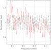 |
Fig. 5 Normalised gain of the ATCA 22 m antennas as function of frequency. The solid curve is the mean gain over all interferometer baselines while the dashed curve is a sinusoid with 20.5 MHz periodicity and 5% peak modulation about the mean. |
2.4. Synthesised beam issues
Some of the influences of the synthesised beam have already been mentioned previously; in particular the far sidelobes of the instantaneous synthesised beam that will be present in an image, due to the residual response of all inadequately modelled sources on the sky. The frequency scaling of the far sidelobe pattern provides significant attenuation of these fluctuations once broad-band frequency averaging has been applied. Another issue in this area is the quality of (u,v) coverage in relation to the sky brightness distribution that requires modelling; both its main-beam and off-axis components. If the (u,v) coverage is inadequate, for example due to a dearth of short interferometer spacings, this will introduce a limitation on the fidelity of the self-calibration model that is deduced, for example via spurious source components, which in turn will limit the precision of the solution. An interesting challenge to consider in this regard is the Sun, with its 106 Jy, 30 arcmin disk and intermittent active regions. If the far sidelobe antenna response does not provide sufficient suppression of this source, it will constitute a significant modelling challenge in any self-calibration solution, as already demonstrated in Fig. 3. Of more general concern is the challenge of modelling sources within the main beam of an observation that are only partially resolved by the synthesised beam. From Table 1 it is clear that the typical sources encountered randomly in a self-cal context are unlikely to be point-like in nature, but rather partially extended for baselines exceeding a few km. Such sources provide a particular modelling challenge, since intrinsic source structure must be distinguished from the general image-plane smearing effects induced by imperfect calibration of the visibilities. An estimate of the maximum modelling error can be made from the Gaussian decomposition of the Cygnus A power spectrum shown in Fig. 1. The fine-scale substructure within this powerful radio galaxy accounts for between 10 and 30% of the total flux. This suggests that a modelling error, ϵM > 0.1, might be the consequence of simply using a point-like model for such sources.
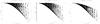 |
Fig. 6 Comparison of input (left) and reconstructed (centre, right) visibilities of a 100 mJy Cygnus A, when observed on-axis in the marginally resolved regime (8 arcsec source size and 12 arcsec beam) with negligible time and bandwidth smearing. The model visibilities in the right hand panel were constrained to only positive source components. The mean visibility error is 0.7% (centre) and 7% (right) relative to the integrated flux of the source. |
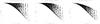 |
Fig. 7 Comparison of input (left) and reconstructed (centre, right) visibilities of a 100 mJy Cygnus A, when observed significantly off-axis in the marginally resolved regime (8 arcsec source size and 12 arcsec beam). The integration time and channel bandwidth were chosen to keep smearing below 10% of the synthesised beam at the edge of the main beam. The model visibilities in the right hand panel were constrained to only positive source components. The mean visibility modelling error is 0.9% (centre) and 10% (right). |
We have attempted to better quantify source modelling errors by considering the quality of a CLEAN reconstruction of Cygnus A when it has been assigned an integrated flux of 100 mJy and an angular size of 8 arcsec and is observed for 12 h with the VLA in the C configuration in a single spectral band at 1.4 GHz. The noiseless input and reconstructed visibilities for an on-axis source location are contrasted in Fig. 6. Realistic thermal noise was included in the imaging and deconvolution process but no additional calibration errors, implying that this is in many ways a best case scenario. Two versions of the reconstructed visibility amplitudes are shown, one in which both positive and negative apparent brightness components found in a CLEAN deconvolution are retained and the other in which only positive brightness components were retained. The input and derived model visibilities have a mean difference of ϵM = 0.007 when all components are retained, but this increases to ϵM = 0.07 when only positive components are permitted. The positive source component constraint has historically been used as a means to discriminate against the inclusion of instrumental calibration errors into the source model that is used for self-calibration. The large modelling errors which arise from this constraint are cause for substantial concern. The unphysical nature of the negative source model is apparent in the visibility amplitudes seen in the centre panel of Fig. 6 which peak at a finite radius rather than at the origin. Despite the unphysical nature of such a source model, it provides a significantly better match for the source visibilities at locations where they have been measured.
When the same source is observed significantly off-axis, by 15 arcmin (a half beamwidth) in both RA and Dec, using a channel bandwidth and integration time that keep smearing effects in this configuration below 10% of the synthesised beam at the main beam edge: Δν/ν = 10-3 and τ = 10 s, the modelling errors increase as seen in Fig. 7. The mean visibility errors increase to 0.9% and 9%, for the unconstrained and constrained cases.
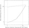 |
Fig. 8 Mean source modelling error as function of the relative visibility smearing scale on the main beam flank. The reference smearing scale is taken to be 10% of the synthesised beam at half power of the main beam. The solid curve is a high precision model that likely represents a best case scenario, while the dashed curve is a simple model that is constrained to have only positive components. |
The unconstrained modelling error increases with larger visibility smearing timescales, reaching 12% for integration times of τ ~ 160 s (while Δν/ν is fixed at 10-3). When the positivity constraint is invoked, this effect dominates over smearing errors until τ ~ 120 s.
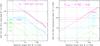 |
Fig. 9 Mean integrated flux density per unit area (left) due to the extragalactic sky and the corresponding number density of flux-weighted source components (right) as function of angular scale. The total is given by the solid curve, while individual bins from Table 1 are plotted as short-dashed curves. |
The magnitude of the modelling error increases approximately linearly with the smearing scale as illustrated in Fig. 8. Background sources dominated by a compact flat spectrum core would be more likely to be modelled accurately, at least when the dominant component is placed exactly on an image pixel. However, the vast majority of random field sources encountered at GHz frequencies are not of this type. The resulting visibility modulation is given approximately by,  (41)where a linear scaling with self-cal solution timescales and frequency intervals (τS,ΔνS) is introduced relative to the nominal intervals (τ⋆,Δν⋆) that keep smearing effects below 10% of the synthesised beamwidth in Eqs. (5) and (6). A typical attenuation of 0.7 for the brightest field source on the main beam flank is also assumed. We will also consider the case where a high precision source model is available from other sources, in which case the residual modelling error,
  , need not scale with the smearing scale,
  (42)This circumstance might arise, for example, if a previous high quality model of the field were available, or the field were fully sampled with the overlapping primary beams of a phased array feed and visibility smearing effects were explicitly included when undertaking data comparison during self-calibration. The number of independent time and frequency samples at this off-axis distance are given by,
  (43)and
  (44)Significant research on better source modelling methods (e.g. Yatawatta 2010, 2011) will be vital to allowing such high precisions to be achieved.
2.5. Self-cal parameters
 |
Fig. 10 NVSS 1.4 GHz source counts (left) per 0.5 dex bin are shown as the filled points connected by a solid line. The analytic approximation over the range 0.003 < S1.4 < 3. Jy that is given by Eq. (47) is overlaid as the dashed curve. The median source size from Table 1 overlaid with an analytic approximation is shown in the right hand panel. |
The signal-to-noise ratio obtained within a self-cal solution interval depends crucially on both the integral source flux density available and the number of flux-weighted components over which it is distributed as demonstrated by Eq. (2). The NVSS statistics of Table 1 and the Cygnus A power spectrum of Fig. 1 were used to calculate the integrated flux density per unit area together with the sum of flux-weighted component number shown in Fig. 9. The solid line in the figure gives the total flux per square degree due to sources between 3 and 300 mJy at 1.4 GHz (for which the likelihood of occurrence in a one degree field is at least unity) while the dark dashed line includes brighter sources as well. Contributions to the integral are quite evenly split between the 10, 30 and 100 mJy bins, while contributions to component number are dominated by the faintest flux bins. As noted previously, source populations are likely to be dominated by luminous radio galaxies (like Cygnus A) above about 30 mJy, while edge-darkened radio galaxies are more likely to dominate below this flux, implying that some modification of our power spectrum template might be appropriate for the faintest flux bins. A representative expression for the integrated flux density per unit area is,  (45)where the total brightness scales roughly as ν-0.8, and the baseline length is normalised to the break at about BR = 10(ν/1.4 GHz)-1 km, below which the total flux saturates. The corresponding expression for flux-weighted major component number is,
 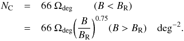 (46)Other important quantities needed to assess the magnitude of many contributions to the visibility noise budget are SMax(Ω), the maximum source brightness that can be expected by chance in a field of a given solid angle together with its overall angular size, ψ in arcsec. The NVSS source counts of Table 1 can be approximated very well with the arbitrary analytic form,
 ![\begin{equation} \label{eqn:nofs} {\rm log}(N({>}S)) = 2.24 - {[{\rm log}(S_{1.4~{\rm GHz}})+5]^{2.4}\over 13.9} \end{equation}](/articles/aa/full_html/2013/03/aa20257-12/aa20257-12-eq185.png) (47)which is overlaid on the count data in Fig. 10 and agrees within 0.02 dex over the range 0.003 < S1.4 < 3. Jy. The median source size, ψ, of Table 1 is also plotted in Fig. 10 together with an analytic approximation,
(47)which is overlaid on the count data in Fig. 10 and agrees within 0.02 dex over the range 0.003 < S1.4 < 3. Jy. The median source size, ψ, of Table 1 is also plotted in Fig. 10 together with an analytic approximation, ![\begin{eqnarray} \label{eqn:pofs} {\rm log}(\psi) & = & 0.31 + 0.27 \left[{\rm log}(S_{1.4~{\rm GHz}})+3\right] \\ [-1mm] \nonumber & \quad + & 0.74\ {\rm exp} \left\lbrace-2 \left[{\rm log}(S_{1.4~{\rm GHz}})-1.3\right]^2\right\rbrace \end{eqnarray}](/articles/aa/full_html/2013/03/aa20257-12/aa20257-12-eq186.png) (48)that agrees with the data to within 0.05 dex. Equation (47) can be inverted to yield the flux of the brightest 1.4 GHz source occurring in a solid angle Ωdeg, as,
(48)that agrees with the data to within 0.05 dex. Equation (47) can be inverted to yield the flux of the brightest 1.4 GHz source occurring in a solid angle Ωdeg, as, ![\begin{equation} \label{eqn:smaxp} S_{1.4 {\rm Max}} = 1.4 \!\times \!{\rm antilog}_{10}(\left\lbrace 13.9 [2.24-{\rm log}(1/\Omega_{\rm deg})]\right\rbrace^{0.417}-5)~{\rm Jy}, \end{equation}](/articles/aa/full_html/2013/03/aa20257-12/aa20257-12-eq187.png) (49)where the leading factor of 1.4 accounts for the median flux of sources within the 0.5 dex bins used in the source counts. This can be scaled to other observing frequencies and baseline lengths via,
(49)where the leading factor of 1.4 accounts for the median flux of sources within the 0.5 dex bins used in the source counts. This can be scaled to other observing frequencies and baseline lengths via, 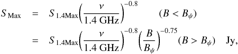 (50)where the characteristic baseline Bψ, that resolves the source is given by,
 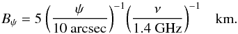 (51)
(51)
Measured and assumed telescope parameters.
2.6. External calibration
There are instances where self-calibration may not be practical and others where it may not even be necessary. It is useful to define the base noise level due to main beam sources under these circumstances. For a gain error of magnitude, φC, with a correlation timescale, τC and fractional correlation bandwidth (Δν/ν)c = δC, we can write the visibility noise associated with a source in the main beam as, 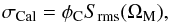 (52)together with the number of independent time and frequency samples in a full track observation as,
  (53)and
 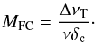 (54)In the event that the main beam field of view approaches 200 deg2, the large field version of the visibility fluctuations, , must be considered yielding,
 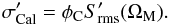 (55)
(55)
3. Some practical examples
With all of the quantities and scaling relationships defined in Sect. 2, it becomes possible to characterise the calibration challenges faced by specific antenna systems. Although the principles we outline are completely general, the source statistics and properties we model are based on data obtained near 1.4 GHz and will be most relevant to frequencies between about 100 MHz and 5 GHz. Outside of this range, there may be significant differences in the source population (e.g. Scaife & Heald 2012; Massardi et al. 2011).
In the subsections that follow, the attributes of several existing and planned arrays listed in Table 2 will be considered, both in terms of visibility noise contributions at the basic self-cal solution interval, as well as the final image noise contributions in an observation of a random field that is tracked for τT = 12 h in the case of a dish array or τT = 4 h for the case of aperture arrays. For the full-track case we will consider both a standard continuum mode observation, in which we assume that a total fractional bandwidth of ΔνT/ν = 0.1 is ultimately averaged together as well as a standard spectral line mode observation in which a spectral resolution of ΔνT/ν = 10-4 is utilised in the image. For the self-cal solution interval, it will be important to achieve a signal-to-noise ratio that is sufficient to allow convergence to be achieved. We will define this by requiring a residual calibration error, as given by Eq. (2), of φ(τS) < 0.5 rad. This yields a visibility solution noise limit, 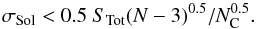 (56)For the full-track continuum imaging it will be of relevance to compare the final image noise contributions with the source confusion level. Condon et al. (2012) have recently estimated the magnitude of such confusion due to the faint source population to be,
 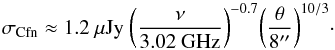 (57)For the purposes of illustration we will consider several examples of main beam source modelling errors, one in which significant effort has been expended to achieve a nominal precision ϵM = 0.01, a cruder version
  and finally a high precision variant,
  . To simplify the interpretation, we will not apply additional scaling of these values with the smearing factors of Eq. (41). Recall from Sect. 2.4 that a 1% precision was found challenging to achieve for marginally resolved background sources with a realistic degree of complexity and that a 10% error was often encountered in practise with simplistic modelling approaches. Achieving 0.1% modelling precision represents a major technical challenge that would rely both on more extensive information of the field under study than is typically available as well as the algorithm complexity to utilise that information effectively. The full track cases will also be compared with the baseline noise level due to gain calibration errors of main beam sources to illustrate the consequence of not applying self-calibration at all. A nominal gain error of φC = 0.2, corresponding to 10 degrees of phase, a correlation timescale of τC = 15 min and a correlation fractional bandwidth of δC = 0.1 will be assumed throughout for illustration purposes. All of the relevant parameters are collected and defined in Table 3.
Of further interest is an answer to the question: “what is the ultimate limit to image noise contributions that follows from multiple long duration tracks of the same field?”. The answer follows from considering which of the error terms are correlated over multiple observing tracks and which are not. The thermal contribution σT, will clearly be uncorrelated from one track to the next. For each of the other contributions we have considered, this is not guaranteed. If the same model is being employed to determine the self-calibration variables for all data tracks, then residual errors due to model imperfections will be identical at the corresponding hour angles of subsequent tracks and the σM component will not average down. In the case of pointing errors, σP, which have not been modelled, it will depend upon the nature of these errors. If they are the result of an incomplete pointing model or diurnal temperature variations they may well approximately repeat on subsequent days. If instead they are due to more random variations such as wind buffeting, they will average down. The contributions due to main beam frequency modulation, σB, as well as unmodelled sources both within near-in, σS, and far sidelobes, σN, are intrinsic to the sky-telescope system and as such will repeat exactly for multiple tracks and will not average away. An exception to this is the case of far side-lobe pickup of the Sun, σD, which will have a different relative location and hence different visibility response on subsequent observing dates. The nominal initial calibration error, φC, is not likely to be correlated between observing sessions if it is dominated by ionspheric or tropospheric phase fluctuations.
Parameter definitions.
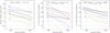 |
Fig. 11 Noise budget for the JVLA-D configuration for a single solution interval (left) for a full track continuum observation (centre) and for a full track spectral line observation (right). Individual noise contributions are as defined in the text. |
3.1. The JVLA
Let’s first consider the JVLA, with its N = 27 (alt,az) mounted dishes of d = 25 m. The logarithmic three-arm “Y” of the JVLA has a high central concentration of baselines in each of its configurations (see Fig. 25-4 of Hjellming 1989) so that more than half of all baselines are within BMed = BMax/6. The four standard configurations, designated (A, B, C, D) are defined by BMax = (36.4,11.1,3.4,1.03) km. The recently upgraded Cassegrain receivers provide continuous frequency coverage with a series of approximately octave band feeds between about 1 and 50 GHz with a system equivalent flux density, 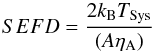 (58)in terms of the Boltzman constant, kB, the system temperature, TSys, the physical area of a dish, A, and the aperture efficiency, ηA. Online JVLA documentation suggests,
 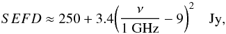 (59)that applies to 1 < ν < 15 GHz, yielding a visibility thermal noise per polarisation product,
 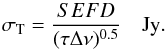 (60)Pointing errors of the VLA 25 m dishes have an rms magnitude of about P = 10 arcsec under good nighttime conditions, that is likely correlated over timescales of about τP = 15 min. The pointing errors have a larger amplitude under daytime and high wind conditions, sometimes exceeding an arcminute, but can also be very effectively reduced under good conditions by a reference pointing strategy to better than about 5 arcsec. Beam squint of the JVLA main beam has been accurately measured (Uson & Cotton 2008) and would contribute ϵQ = 0.055 if not modelled in an observation. The magnitude of main beam modulation with frequency of the VLA has not been documented, but the similarity in feed geometry to that of the ATCA suggests that a comparable value of ϵB = 0.05 will likely apply when this modulation is not explicitly accounted for in the self-calibration process. The primary-subreflector separation is, lC = 8.2 m. The near-in sidelobe level of the main beam is about 2%, so ϵS = 0.02, if such sources, including their apparent time variability are not accounted for in the self-cal model of the field. In view of the significant azimuthal variation in the sidelobe properties, and their rotation with parallactic angle, accounting for these effects adds substantial complexity to the processing (e.g. Bhatnagar et al. 2008). The far sidelobe contributions under daytime, σD, and nighttime, σN, conditions follow directly from the dish diameter and Eq. (4), which has been calibrated with ηF = 0.1 from Dhawan (2002) and Eqs. (14) and (13). The magnitude of the residual source modelling errors will depend on the methods and effort that have been employed to minimise these effects.
The noise budget for the JVLA in its D configuration is shown in Fig. 11. On the solution timescale appropriate to keep smearing effects below 10% of the synthesised beamwidth the thermal noise, σT, is below that which is required for self-cal convergence σSol. This implies that full-field self-cal can be performed with minimal smearing effects. As will become apparent below, this condition is often not met in practise by telescope systems, so that more extensive data averaging becomes necessary. The thermal noise is seen to dominate over all noise contributions except for daytime observations below about 1.4 GHz, where visibility modulation by the Sun becomes comparable. A full track continuum observation is dominated by source confusion noise, σCfn, below about 1.5 GHz. However, the calibration noise, σCal, vastly exceeds the thermal noise and becomes dominant overall at higher frequencies, implying a clear need for self-calibration. The next largest contributions come from source modelling errors (in the case,  , where only 10% precision is achieved), followed by beam squint σQ, near-in sidelobe σS and main beam modulation σB. Sky-limited continuum performance above about 2 GHz will rely on achieving a high source modelling precision and explicit beam squint compensation. In the case of a full track spectral line obervation, the thermal noise is seen to dominate above 2–3 GHz, although self-calibration will be necessary at lower frequencies. Solar modulations will have a negative impact on daytime spectral line performance at frequencies below about 1.5 GHz. Ultra-deep spectral line observations will ultimately become limited by the stationary error contributions as noted above. The most important of these are , σS, σB and σQ. Even so, it should be possible to improve upon the single track sensitivity by about a factor of several in long integrations, provided the source modelling precision is better than about 3% and most importantly, that RFI is negligible.
The same type of analysis applied to the JVLA-C configuration is given in Fig. 12. Here we see that while the thermal noise dominates over other contributions on the desired solution timescale, it exceeds what is required for self-cal convergence σSol, so that more extensive data averaging, by about a factor of two in both domains, becomes necessary. This will imply more extensive time and bandwidth smearing for off-axis sources, which may limit the source modelling precision which can routinely be acheived. The full track continuum observation will require self-calibration to reach the thermal noise. Substantial effort needs to be expended on achieving a source modelling precision approaching 1%, otherwise this contribution will dominate the noise budget below 3 GHz. The next most serious effect is that of beam squint. As noted previously, active modelling of this effect has proven effective at improving image dynamic range at the expense of computational complexity (Uson & Cotton 2008). By addressing both of these issues satisfactorily it should become possible to reach the thermal noise. Reaching the source confusion level σCfn in deep integrations will be considerably more challenging, since several additional error contributions would need to be overcome. The full track spectral line observation is thermal noise limited above 2–3 GHz, while self-calibration with at least moderate source modelling precision (<10%) will be required at lower frequencies. Even deep integrations should still be in this regime, provided that RFI remains negligible.
Very similar patterns are seen in the more extended B and A configurations as shown in Figs. 13 and 14. The more extended configurations require smaller time and frequency averaging intervals to support the iterative full-field source modelling inherent to self-calibration, but the finite sensitivity per visibility does not allow this to be achieved while providing enough signal-to-noise. Excess averaging in both domains by about a factor of five (and ten) are required for the B (and A) configuration(s). This will severely impair the ability to achieve high levels of modelling precision on the main beam flanks for the simplest imaging algorithms. More complex wide-field imaging and modelling strategies will be mandatory under these circumstances, such as employment of multiple distributed phase centres. While such methods are well-understood, they impose a significant computational overhead. The full track continuum performance relies on self-calibration and beam squint effects will also need to be addressed to reach the thermal noise. Source modelling precision better than about 1% will be required, together with explicit modelling of the full range of main beam and near-in sidelobe effects (σQ, σP, σB and σS) if deep integrations are to remain in that regime. The challenges in all these areas are greatest at the lowest frequencies and for the less extended configuration.
3.2. ATA
The Allen Telescope Array (Welch et al. 2009; Harp et al. 2011) consists of N = 42 off-axis (alt,az) mounted dishes of d = 6.1 m. The ATA configuration is very compact with BMax = 323 m and BMed = 81 m. The dishes are fed by an ultra-wideband log-periodic feed from a Gregorian focus over the frequency range 0.5 to 10 GHz. A model for the system temperature performance of the system as function of frequency presented by Welch et al. (2009) provides,  (61)in terms of the frequency in GHz, νG, at an assumed aperture efficiency, ηA = 0.6. Typical values of receiver temperature and illumination efficiency tabulated by (Harp et al. 2011) suggest significantly higher values of TSys/ηA between about 70 and 270 K. The values of TSys given by Eq. (61) range between about 37 and 60 K, with corresponding SEFDs between 5800 and 9400 Jy. The pointing accuracy of the dishes under good nighttime conditions is P = 90 arcsec with a likely correlation timescale τP = 15 min. The beam squint for this offset design has been measured (Harp et al. 2011) to be about 4% FWHM at 1.4 GHz, yielding ϵQ = 0.04. Major asymmetries in the main beam shape, at the 20% level, are also documented graphically by Harp et al. (2011), suggesting that a beam squash contribution to ϵQ may be significantly larger. The peak near-in sidelobe levels measured at 2300 MHz are about 1%, yielding ϵS = 0.01, with substantial azimuthal variation in sidelobe intensity. While beam and sidelobe modulation with frequency have not been documented directly, they might be expected to track the gain modulation with frequency intrinsic to the log-periodic feed, which has an rms fluctuation level of about 1 dB, or
  and correlation bandwidth, Δν/ν ≈ 0.03. This particular gain modulation is due to the quantised, resonant element wavefront sampling of the wide-band feed and is in addition to any multi-path induced gain modulation with frequency as discussed previously. Multi-path beam modulation should have a much lower amplitude, of perhaps ϵB ≈ 0.01 (twice the GBT value). Since the feed is mounted on the edge of the primary reflector surface, the primary-subreflector separation of about lC ≈ 3 m is likely the most relevant cavity dimension for an estimate of modulation periodicity. For the purpose of our analysis, we will consider both of these possibilities for main beam modulation ϵB. Harp et al. (2011) have also carried out far sidelobe measurements of the ATA dishes at 2300 MHz which are in the range of –30 to –40 dB over much of the sky. This implies a value of ηF = 0.7 for use in Eq. (4) which is significantly higher than that which applies to the upgraded JVLA.
The noise budget analysis for the ATA telescope is shown in Fig. 15. What is striking is that visibility fluctuation levels are predicted to be completely dominated by the far sidelobe response on the self-cal solution timescale. During daytime observing this is true up to 3 GHz, while even for nighttime observing this will be the case below 1.4 GHz. This is a consequence of both the small dish size and the very compact array configuration. Substantial visibility averaging (by about a factor of five in both domains) would diminish these contributions to the point that the self-cal signal-to-noise criterion could be met. A full track continuum observation would be source confusion noise limited, but many of the noise contributions under consideration would exceed the thermal noise below about 1 GHz. Above 1 GHz, the potential main beam modulation associated with gain variations of the wide-band log-periodic feed becomes the most important contributor for nighttime observations. The full track spectral line case is dominated by far sidelobe effects below a few GHz. The nominal calibration noise exceeds the thermal noise below about 1 GHz, implying that self-cal may not be required for spectral line applications at higher frequencies. In that case, it may be possible to simply ignore the far sidelobe response contributions, since the visibility gridding function will provide some 40 dB of suppression for such distant sources. Any sidelobes of the instantaneous synthesised beam response will of course not be suppressed during imaging which may become a limitation in this case. Deep spectral line integrations would encounter a range of issues that would necessitate extensive modelling and self-calibration to overcome.
3.3. ASKAP
Let us now consider what challenges will be faced with the ASKAP array, with its N = 36, three axis (alt,az,pol) mounted dishes of d = 12 m. The ASKAP configuration is highly centrally concentrated with BMax = 6 km and BMed = 630 m. The dishes are fed with a prime focus PAF (phased array feed) that covers the frequency range 700 to 1800 MHz. Current performance estimates are for TSys/ηA = 55 K across this band, yielding an SEFD of 1340 Jy for the 12 m dishes.
Mechanical pointing errors of the ASKAP dishes under normal operating conditions have not yet been determined, but will be assumed to be about P = 10 arcsec under good nighttime conditions and correlated over timescales of about τP = 15 min. What must also be assessed is the electronic pointing error that might be associated with gain fluctuations of the individual antenna elements that are combined to produce the main beam in a PAF. While actual values have not yet been determined, current estimates of the element gain variability are better than  with variability timescales of
  min.
min.
The main beam modulation phenomenon that afflicts single-pixel-fed radio telescopes has been demonstrated to be diminished by between 20 and 30 dB in a PAF system (Oosterloo et al. 2010) employing Vivaldi antenna elements. The reason for this improvement appears to be related to a much better and physically more extended power matching to the incident radiation field, such that reflectivity from the feed is minimised. While similar measurements are still required for the chequerboard antenna array of the ASKAP phased array feeds, it is expected that they will have similar performance in this regard. We will assume a conservative 10 dB reduction in the frequency modulation, to ϵB ≈ 0.005.
The phased array feed also provides the potential to strongly suppress beam squash through optimisation of the individual polarisation beams and their relative alignment. Furthermore, as noted previously, the ability to track parallactic angle with the “polarisation” axis allows any residual beam squash pattern to be fixed on the sky during tracking so that the apparent brightness of sources on the beam flank remains unchanged. For illustration purposes we will assume a 10 dB reduction due to each of these contributions to beam squash from a base level that would apply to an (alt,az) mounted single pixel feed of 4%, giving ϵQ = 0.0004.
The near-in sidelobe pattern of a phased-array feed illuminated reflector is expected to have a comparable near-in sidelobe level to that of the single-pixel-fed equivalent (Oosterloo et al. 2010), so is likely to have a peak amplitude of some 2%. However, unlike the single-pixel-fed counterpart, this pattern is not expected to display an amplitude modulation with frequency. As noted above for the main beam modulation, the phased array feed illumination pattern is expected to be very similar over frequency rather than modulated at the 5% level. Moreover, the polarisation rotation axis of the ASKAP telescope mount will permit all of the telescope sidelobes, including the radial spokes associated with the prime focus support struts, to remain stationary on the sky during source tracking. The time and frequency stability of the near-in sidelobe response would enable straightforward modelling of sources at these large offsets. Furthermore, it is planned that all 36 digital main beams formed by the PAF will be processed simultaneously via a joint self-cal source model for the entire field of view. The implication is that source information for modelling the field of each main beam and its near-in sidelobes is provided by a beam in which that source is essentially on-axis, with minimal smearing effects or main beam attenuation. Provided that the relevant time and frequency smearing effects for each beam are explicitly included during data comparison, it should permit very low values of both ϵS and ϵM to be obtained. For illustration purposes, we will assume only a conservative 10 dB reduction in this component to ϵS = 0.002.
For the far sidelobe contributions under daytime, σD, and nighttime, σN, conditions we will assume ηF = 0.1 since we expect excellent illumination quality in this prime focus system, comparable to what currently applies to the Cassegrain JVLA and the prime focus WSRT together with Eqs. (4), (14) and (13). This represents an improvement by perhaps a factor of 2 relative to a single pixel fed dish of this size.
The noise budget analysis is presented in Fig. 16. Thermal noise is seen to dominate on the self-cal solution interval, although the signal-to-noise requirement implies that additional data averaging (by about a factor of five in both domains) is needed. The full track continuum case demonstrates that self-calibration will be essential and that source modelling errors will be the single most important factor to address for this array design. For single track observations, these must be kept below about 1% to achieve thermal noise limited performance, but for deep integrations above 1 GHz, it will be necessary to achieve even better precision in order to reach the source confusion level. As noted above, the simultaneous imaging of the multi-beam field-of-view offers good prospects for achieving high source modelling precision. It is also of interest to compare the contributions of electronic,  , and mechanical pointing, σP, to the noise budget in this case. While these contributions have different frequency scalings, they have a similar magnitude for the parameters assumed here. It is also worth noting that the electronic component is not expected to be correlated over multiple observing sessions, so will average down further in a deep observation. The full track spectral line case should permit routine thermal noise limited performance to be achieved, although self-calibration is required across the band. Deep spectral line integrations will become dependent on the quality of source modelling.
3.4. MeerKAT
MeerKAT is currently planned to consist of N = 64 off-axis (alt,az) mounted dishes of d = 13.5 m (Booth & Jonas 2012). A single Gregorian focus feed covering about 1 to 1.74 GHz is planned for the first phase of deployment with a specified total sensitivity of about 220 m2/K, corresponding to TSys/ηA ≈ 42 K and an SEFD of 810 Jy. While the telescopes have not yet been fabricated, we will assume that relatively good pointing accuracy of about P ≈ 10 arcsec may be realised under good conditions with a correlation timescale τP ≈ 15 min. Beam squint for the MeerKAT dishes is expected to be somewhat larger than that of the GBT, given the smaller size of the subreflector of about 4 versus 7.5 m, so may be about ϵQ ≈ 0.01 in practise. Beam squash simulations are not available, so we will assume that values comparable to those achieved at the GBT will apply of ϵQ ≈ 0.04. Peak near-in sidelobe levels will depend on the degree of edge illumination, but might be about ϵS ≈ 0.01. Similarly, the multi-path induced beam modulation effects might also be slightly larger than those of the GBT, ϵB ≈ 0.01, while the dominant resonant “cavity” dimension in the system will probably be the primary-subreflector separation of about lC ≈ 7 m. The recent study of Cortes & Imbriale (2009) provides an indication of far sidelobe levels from similar optical designs and dish dimensions of about –40 dB at 1.4 GHz. This would suggest ηF ≈ 0.5 for use in Eq. (4). However, the Cortes & Imbriale (2009) study used the non-optimum illumination of an ultra-wideband feed and is strongly influenced by subreflector spillover. An octave band Gregorian feed design is more likely to achieve superior illumination quality of perhaps ηF ≈ 0.2. The MeerKAT array configuration will have BMax = 8 km, but be highly centrally concentrated with BMed ≈ 500 m.
Inspection of the noise budget analysis in Fig. 17 shows that more substantial data averaging (by about a factor of four) is required to meet the σSol criterion in the self-cal solution interval. For the full track continuum case, self-calibration is clearly required and the subsequent noise budget is completely dominated by source modelling errors. Reaching the thermal noise in a single track will require achieving better than about 1% modelling precision, which will be challenging. Beam squash effects constitute the next challenge, with these contributions exceeding the thermal noise by factors of several. Explicit modelling of the time variable response in the elliptical polarisation beams will be essential to achieving thermal noise limited performance. Comparison with the JVLA plots for similar configurations in Figs. 12 and 13, suggests that it will be about twice as challenging for MeerKAT to achieve thermal noise limited performance as the JVLA.
Achieving even lower noise levels in deep integrations will require a significant further reduction in the source modelling and beam squash errors, together with explicit modelling of additional main beam and near-in sidelobe issues (σP, σB and σS). The full track spectral line analysis suggests that thermal noise limited performance will be straightforward to achieve provided self-calibration is employed, with deep integrations becoming sensitive to the precision of source modelling.
3.5. SKA1-Mid
The Square Kilometre Array Organisation has recently announced the intention that the SKA Phase 1 mid-frequency dish array be deployed as two complimentary components: an SKA1-Survey instrument to be sited in Australia and an SKA1-Dish array to be sited in South Africa.
3.5.1. SKA1-Survey
The SKA1-Survey instrument is projected to consist of N = 96 dishes of d = 15 m covering the frequency band of 0.45–3.0 GHz with three overlapping phased array feed systems, each of octave bandwidth. While the array configuration has not been determined in detail, it might be expected to have BMax = 20 km and BMed = 1 km. The sensitivity specification calls for TSys/ηA = 50 K above about 1 GHz, accepting the fact that the Galactic contribution will become significant at lower frequencies. An estimate of the frequency dependence of system performance is given by, 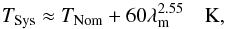 (62)in terms of a nominal temperature, TNom (that excludes the Galactic contribution) and the wavelength, λm in meters. Relevant values for the PAF systems might be TNom = 37 K and ηA = 0.8. An antenna and mount design have not yet been determined for the SKA, but for the present purpose we will assume that an off-axis Gregorian-fed system with an (alt,az) mount is utilised. We will assume good mechanical pointing accuracy of about P ≈ 10 arcsec with a correlation timescale τP ≈ 15 min. Electronic pointing errors of correlated over min will also be assumed. In the absence of a polarisation mount axis, it will be necessary to track the digital PAF beams which are offset from boresight across the focal plane. The substantial intrinsic beam squash of about 4% is likely to be improved by about 10 dB with polarisation specific PAF illumination to about ϵQ = 0.004. The multi-path induced beam modulation will be decreased from its nominal 1% level in such an off-axis design by at least 10 dB to ϵB ≈ 0.001. Near-in sidelobes ϵS ≈ 0.01 will be assumed in this offset design. Good quality PAF illumination should provide an improvement of about a factor of two in the far sidelobe efficiency to ηF = 0.1.
The self-cal solution noise budget in Fig. 18 demonstrates yet again that there is insufficient sensitivity for self-calibration at the “natural” time and frequency interval for straightforward, full beam imaging, necessitating some further data averaging. The full track continuum case will require self-calibration and significant attention to source modelling, particularly at the lowest frequencies where a precision of <1% will be required, with the near-in sidelobes representing the next largest error contribution. It is the absence of a polarisation axis which introduces time variability into the near-in sidelobe response and adds this complexity to the imaging problem. Obtaining very deep integrations will rely on further precision in modelling sources both in the time variable near-in sidelobes as well as in the main beam. Full track spectral line observations are expected to be much more straightforward, although they will require self-calibration. Deep integations will become limited by source modelling precision.
3.5.2. SKA1-Dish
The SKA1-Dish array is projected to consist of N = 250 dishes of d = 15 m covering the frequency band of 0.45–3.0 GHz with three overlapping single pixel feed systems, each of octave bandwidth. The array configuration is expected to extend out to BMax = 100 km but maintain a BMed ≈ 1 km. However, to simplify comparison of the results with both SKA1-Survey as well as the more extended configurations of the JVLA, we will only illustrate the case of BMax = 20 km. The single pixel feed sensitivity specification calls for TSys/ηA = 44 K above about 1 GHz. Relevant values for use in Eq. (62) might be TNom = 28 K and ηA = 0.7. The mechanical pointing errors assumed above will apply with P ≈ 10 arcsec and a correlation timescale τP ≈ 15 min, as well as the near-in sidelobe response of ϵS ≈ 0.01. A beam squash of ϵQ ≈ 0.04 and multi-path modulation of ϵB ≈ 0.01 with lC ≈ 7 m such as discussed for MeerKAT are also likely to be relevant here. A far sidelobe response of ηF = 0.2 is assumed to apply for the likely dish illumination quality.
The thermal noise is just sufficient to permit self-cal convergence on the “natural” solution interval at the bottom end of the frequency coverage, but exceeds that limit above about 600 MHz. A full track continuum observation will require self-calibration and will need to achieve high precision source modelling in the main beam, varying between about 0.3 and 3% from the bottom to the top of the band. The beam squash effects must also be actively modelled in order to permit the thermal noise limit to be achieved. Deep integrations would only approach the source confusion limit if a range of additional effects were effectively modelled, including the near-in sidelobes and main beam modulation. Full track spectral line observations will require self-calibration, but are only moderately sensitive to the source modelling precision.
3.6. LOFAR high band
The LOFAR array (Heald et al. 2011) consists of stations distributed over much of the Netherlands as well as in other European countries. For the purpose of our analysis we will consider only the LOFAR High Band that covers frequencies between 120 and 240 MHz and the stations within NL. It will be useful to consider both the core configuration of N = 48 stations of d = 30.75 m diameter for which BMax = 3.5 km and a core plus remote configuration with a total of N = 64 stations and BMax = 121 km. While the remote stations have a larger physical size than those in the core, we will assume that only the central d = 30.75 m of these outer stations is utilised to simplify their combination with the core stations during imaging. The configuration of stations is highly centrally concentrated with a baseline density that declines roughly as B-2 beyond about 100 m. For the core configuration we will assume BMed = 250 m while for the core plus remote configuration this might increase to BMed = 1 km. The SEFD of the LOFAR High Band core stations is projected to vary approximately as, 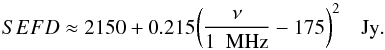 (63)Mechanical pointing errors clearly do not apply to an aperture array. There may well be an electronic pointing error associated with gain fluctuations of the individual antenna elements that are combined to produce the station beam. Actual values are not yet documented but the impact will be assesed by assuming a station beam variability amplitude of about and timescale of min. As was the case for the phased array feed, we expect beam squint and beam squash to be minor, if there is optimisation for these parameters. However, the minimisation of beam squash for an aperture array will require active compensatation of the geometric foreshortening of the stations for the duration of the observing track. While this can be realised it will come at the expense of sensitivity, since the “lowest common denominator” approach for the effective aperture would need to be applied. An alternative to this straightforward strategy would be the use of the “A-projection” algorithm, as outlined previously, to attempt to compensate for the changing, assymetric station beams during an observation. As noted above, this method only provides approximate “forward” correction of the acquired data. Experience on the applicability and precision of this method needs to be acquired and documented. A reference value of ϵQ = 0.01 will be assumed to track the impact of any residual unmodelled beam assymetries. As noted at the outset of this section we will assume that a full track observation has τT = 4 h duration to limit the severity of geometric foreshortening. Main beam modulation due to multipath effects is clearly not relevant to the aperture array geometry, eliminating the ϵB component. The near-in sidelobe amplitude is also open to optimisation with the choice of digital tapering of the station beam weights. However, a lower sidelobe will come at the expense of station sensitivity. For illustration purposes, we will assume a uniform aperture weighting to achieve maximum sensitivity, although this yields a large value of ϵS = 0.1. Measured HBA sidelobe levels are somewhat greater than 10% and are highly modulated with azimuthal angle. The magnitude of the far-sidelobe response of the LOFAR stations is not yet documented. In view of the discrete rather than continuous nature of the aperture sampling, a relatively large value of ηF ≈ 0.5 might be appropriate.
The LOFAR Core configuration noise budget is shown in Fig. 20. At the nominal solution timescale, the thermal noise easily satisfies the self-cal signal-to-noise requirement, σT < σSol. However, the far sidelobe response to both the daytime, σD, and the nighttime sky σN, completely dominate the noise budget by several orders of magnitude. Self-calibration will not be possible without very extensive modelling of the sky for a nominal solution interval (τ⋆,Δν⋆). Comparison with Fig. 2 demonstrates how deep it will be necesssary to go before these contributions will no longer dominate the fluctuation level on a solution interval. The first order of magnitude reduction will be addressed by adequately modelling the 30 brightest sources (per 2π sr) with S1.4 GHz > 30 Jy. Unfortunately, even this may not be sufficient below about ν = 180 MHz. The next flux bin, 10 < S1.4 GHz < 30 Jy, contains an additional 70 sources per hemisphere. With this reduction in fluctuation level (by about a factor of 17) self-calibration should become practical over the entire band. The other method for reducing the far sidelobe fluctuations within a solution interval might be extensive data averaging in time and frequency. As can be seen from Eqs. (13) and (14), increasing each of these by an order of magnitude would provide a factor of ten reduction in the fluctuation amplitude, although at the expense of a major negative impact on the ability to model sources on the main beam flank with precision. In practise a hybrid approach might be employed whereby some number of the brightest sources are modelled directly and the remainder are suppressed by a degree of visibility averaging. The full-track noise budget plot demonstrates that the LOFAR Core will be source confusion limited for continuum observations after only short integrations. Of potential concern is the fact that the thermal noise is exceeded by the majority of other effects under consideration.
The full-track spectral line observation demonstrates the challenges that will be faced by the Epoch of Reionisation experiments (Zaroubi et al. 2012). Self-calibration will be necessary to permit the thermal noise floor to be reached. However, far sidelobe contributions vastly exceed the thermal noise and will require extensive modelling to achieve the necessary 20 to 30 dB reduction. This requirement is significantly more stringent than that encountered on the self-cal solution timescale and will be very challenging to meet in the lower half of the band, where 100’s of sources distributed over the entire sky must be modelled. Unmodelled sources in the near-in sidelobes also lead to excess image noise that exceed σT by factors of several in each four hour track. As noted previously, the near-in sidelobe pattern with uniform aperture weighting is highly modulated with parallactic angle, implying that this time variability will require active modelling. Since both σN and σS are tied to the intrinsic telescope-sky response they will not average down in long integrations. The ultimate noise floor in a deep field observation will be entirely limited by the quality of the sky modelling. It may well be deemed beneficial to employ significant tapering of the station aperture to reduce the near-in sidelobe level. Unfortunately, such aperture tapering may have the undesirable side-effect that the far sidelobe response is further enhanced, since the effective station diameter, d, is reduced.
The noise budget for the combined Core plus Remote configuration is shown in Fig. 21. The nominal solution timescale for this much larger value of BMax does not provide adequate signal-to-noise for self-calibration. A substantial degree (factor 10) of time and frequency averaging is necessary to bring σT down below σSol which will have an adverse effect on source modelling within the main beam. Such averaging will provide attenuation of the far sidelobe contributions by an order of magnitude. Even so, a further reduction of σD or σN by at least another order of magnitude is needed to allow for the possibility of self-cal convergence. As discussed above, a minimum requirement will be modelling and excision of the S1.4 GHz > 30 Jy source category. The full-track continuum noise budget shows that source confusion noise has now become negligible relative to other terms. Unfortunately, there are many error contributions that exceed the thermal noise in a single track and self-calibration is clearly necessary to approach that limit. We will assume that the far sidelobe contributions have been reduced from the outset by about a factor on ten through modelling of the S1.4 GHz > 30 Jy population. The next limitation becomes that of unmodelled sources in the near-in sidelobes, followed by modelling errors associated with main beam sources. Reaching the thermal noise in a four hour track will require a source modelling precision that exceeds 0.3%. This will be particularly challenging in view of the high degree of visibility smearing (factor 10) required to provide solution signal-to-noise. The modelling of the time variable response to sources within the near-in sidelobes will also need to achieve a 1% acccuracy, in order to avoid this potential limitation. It is likely to be very challenging to reach the thermal noise in such four hour tracks. Even deeper continuum integrations would need to improve on all of the previously mentioned error contributions.
The full-track spectral line case is significantly less challenging than the continuum for the Remote configuration, although again self-calibration is required across the entire band. Once the far sidelobe effects have been reduced to the point where self-cal becomes possible, the primary limitation come from adequate modelling of sources within the near-in sidelobes. This must be reduced by about a factor of two to reach σT. Deeper spectral line integrations will need to improve further on the σS component and may then also need to improve on the far sidelobe contributions σN.
3.7. Murchison Wide-field Array (MWA)
The MWA (Lonsdale et al. 2009) is currently expected to consist of N = 128 station tiles, each a square of 4.4 × 4.4 m dimensions that cover the frequency band 80–300 MHz. The configuration is planned to be centrally concentrated with BMax = 3 km and BMed ≈ 300 m. The system temperature is expected to vary as, 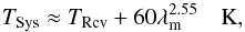 (64)in terms of a receiver temperature, TRcv and the wavelength, λm in meters. While the receiver temperature specification is not currently published, we will assume TRcv = 150 K as a representative value. The effective collecting area per station is expected to vary as,
 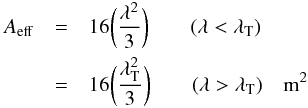 (65)for 16 dual polarisation antenna elements in each tile that are sparsely distributed for λ < λT = 2.2 m. We will assume an electronic pointing error associated with gain fluctuations of the individual antenna elements of about and timescale of min. The rectangular tile geometry will give rise to large departures from axisymmetry for the main beam shape. We will also assume a residual beam squash error of ϵQ = 0.1 that applies to the full track observations of τT = 4 h duration. Untapered aperture weighting is assumed that might yield a near-in sidelobe contribution ϵS = 0.1. The far sidelobe response will be characterised by ηF ≈ 0.5.
The noise budget plot of Fig. 22 demonstrates the regime that this facility will operate in. In view of the extremely large field of view of each tile, that varies between 200 and 3000 deg2 across the band, this is a case where the “quiet” sky approximation is clearly not relevant and Eq. (21) rather than 20 is employed in calculating noise terms. Far sidelobe pickup of the sky will dominate over all other contributions by two to three orders of magnitude on a natural solution timescale. Even full track continuum and spectral line observations are completely dominated by this all-sky response to a similar degree. Comparison with Fig. 2 suggests that even the S1.4 GHz < 0.1 Jy population is contributing to visibility modulations in this regime. Modelling of the time variable response to each of 10 000+ sources on the sky does not seem likely to be practical. Even the 8000 instantaneous visibilities are less in number than the number of relevant sources on the sky, without considering any instrumental variables. Traditional self-calibration is not a viable option in this circumstance, although it appears to be essential to provide some improvement to the noise budget for both continuum and spectral line observations. A telescope operating in this regime will need to rely on the quality of external calibration that can be acheived and seems unlikely to achieve thermal noise limited performance.
3.8. SKA1-Low
The Square Kilometre Array Phase 1 low frequency aperture array is currently expected to consist of 50 stations of d = 180 m diameter operating between 70 and 450 MHz. The array configuration is planned to consist of 25 stations within a diameter of 1 km, a further 10 in the annulus of 5 km diameter and a final 15 distributed out to perhaps 100 km. The system temperature is expected to vary as, 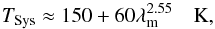 (66)in terms of the wavelength, λm in meters. The effective collecting area per station is expected to vary as,
 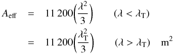 (67)given the 11 200 dual polarisation antenna elements in each station that are sparsely distributed for λ < λT = 2.6 m. Many of the same considerations discussed previously for the LOFAR analysis apply here as well. We will assume an electronic pointing error associated with gain fluctuations of the individual antenna elements of about and timescale of min. We will also assume a residual beam squash error of ϵQ = 0.01 that applies to the full track observations of τT = 4 h duration. As a starting assumption we will assume untapered aperture weighting that yields a near-in sidelobe contribution ϵS = 0.1. The far sidelobe response will be characterised by ηF ≈ 0.5. Just as done for the case of LOFAR we will consider both a core configuration with N = 35, BMax = 5 km and BMed = 500 m, as well as an extended configuration with N = 50, BMax = 100 km and BMed = 2500 m.
The noise budget for the SKA1-Low core is shown in Fig. 23. Although the thermal noise is well below the self-cal solution limit on the natural timescale, there are a number of other contributions that exceed σT by large factors. Far sidelobe pickup is chief among these, followed by near-in sidelobe contributions and source modelling errors. The brightest 10–20 dB of the nighttime sky will likely require modelling to allow useful self-calibration to be undertaken. Full track continuum performance is completely source confusion dominated, while the spectral line case is analogous to that seen on the solution timescale. Self-cal will be required to approach the thermal noise, but far sidelobe modulations dominate by two to three orders of magnitude over the thermal noise, followed by near-in sidelobe sources and source modelling errors. A source modelling precision of about 0.3% is required, once the σN and σS contributions have been reduced to the point that they no longer dominate. Adequate modelling of the nighttime sky will be quite challenging, since its contribution will need to be reduced by about 20 dB below about 120 MHz. As noted previously, this will entail modelling down to the S1.4 GHz < 0.1 Jy level, where more than 104 sources are above the horizon at any moment.
The noise performance of the extended SKA1-Low array is shown in Fig. 24. While some far sidelobe modelling or data averaging is needed to enable self-calibration, this is less extreme than for the more compact core. The full track continuum performance faces a wide range of practical challenges. All of the effects under consideration exceed the thermal noise below 200 MHz; the most severe being unmodelled sources in the near-in sidelobe which must be reduced by some 20 dB. The full track spectral line case is somewhat less challenging, although some 10 dB are required here as well. Self-calibration is required for both continuum and spectral line applications.
4. Discussion
4.1. Dishes
Consideration of the various telescope systems in Sect. 3 allows some general conclusions to be drawn. The “traditional” 25 m diameter class dishes of existing synthesis radio telescopes operate in a regime where the thermal noise of the receiver system dominates the noise budget on a self-cal solution interval, typically by a large margin. Furthermore, at least for relatively compact configurations, there is adequate signal-to-noise provided by sources occurring randomly within the field to allow self-calibration to be undertaken at close to the “natural” solution interval that keeps time and bandwidth smearing effects at a small fraction of the synthesied beamwidth over the entire primary beam field of view. This constitutes the most advantageous of circumstances, since simple imaging strategies can be employed that use only a single version of the data, in contrast to more complex strategies that might require simultaneous processing of multiple phase centres. Even so, full track continuum observations must overcome several potential obstacles, at the 10 dB level, before thermal noise limited performance is achieved below 2 GHz. This is consistent with practical experience with the JVLA, the WSRT and the ATCA where considerable care must be excercised with precise modelling of sources that occur within the field and in the case of the JVLA, explicit modelling of the non-axisymmetric beam shape and its rotation on the sky during tracking, to keep these effects from becoming dominant. Above about 2 GHz and in more extended array configurations it becomes necessary to introduce more data averaging prior to self-calibration than is optimum for simple imaging strategies. However, only a limited number of complications need be addressed to achieve thermal noise limited performance in full-track continuum observations in these circumstances. The full-track spectral line performance of such arrays is less subject to complications and only requires self-calibration to reach the thermal noise floor below about 2 GHz. Only in the most compact configurations and at frequencies approaching 1 GHz does the Sun begin to present some problems.
This is in stark contrast to the situation encountered with synthesis arrays that employ significantly smaller dishes. The most striking comparison is with the ATA, where the combination of small dish diameter and compact array configuration yield a very different regime. For a nominal self-cal solution interval, the thermal noise is dominated by the far sidelobe response to the entire sky. The same is true even after integrating over an entire 12 h track, both for spectral line and continuum applications. Continuum observations are further challenged by a wide range of other noise contributions which dominate over the thermal noise. Its not clear whether high dynamic range imaging in this regime will be possible.
The case of 12 to 15 m class dishes in more extended configurations is improved over that with only 6 m dishes. Even so, more than nominal data averaging is required to provide the signal-to-noise needed for self-calibration with this dish size, which will add complexity to wide-field imaging. Higher source modelling precision than what has been needed for the 25 m VLA dishes, by about a factor of two will be required, together with explicit modelling of any main beam asymmetries in cases where the parallactic angle is not fixed on the sky during an observation. In this respect, the ASKAP telescope benefits from both the greater circular symmetry of polarisation beams possible with a phased array feed as well as the polarisation rotation axis that keeps the beam orientation fixed on the sky during tracking. Single pixel fed systems with an (alt,az) mount will face significantly greater challenges to reach the thermal noise floor. Deep field continuum observations will need to achieve extremely high source modelling precision that extends out into the near-in sidelobe region.
Exactly the same considerations apply to the SKA, if 15 m class dishes are deployed as envisaged within the current baseline design. Achieving thermal noise limited continuum performance will be more challenging than with the 25 m dishes of the JVLA and sub-μJy imaging would need to overcome a whole range of complex modelling issues. One of the greatest threats to thermal noise-limited performance is the departure from circular symmetry of the polarisation beams and the rotation of this pattern on the sky. The use of phased array feeds provides one means of reducing the risk associated with beam asymmetries, while the adoption of an equatorial or (alt,az,pol) mount system provides another for eliminating their time variability.
Adoption of a larger dish diameter would provide a significant risk reduction and this option should be considered very seriously during cost/performance optimsation of the final SKA dish design.
4.2. Aperture arrays
The aperture arrays considered in Sect. 3 display many of the same phenomena. The small station sizes of LOFAR (30.8 m) and particularly the MWA (4.4 m) result in visibilities that are completely dominated by noise-like modulations from sources appearing in the far sidelobe response. Very extensive modelling of the visibility response to these distant sources becomes necessary before self-calibration within the main beam can be contemplated. A major additional complication is introduced by the geometric foreshortening of each station aperture while tracking a source. While an absence of moving parts is often cited as a major advantage of these systems, the continuously changing response of the sky-telescope system is the price that is paid. Efforts are underway to improve predictive modelling of both the far sidelobe response patterns (Wijnholds et al. 2010) as well as compensation for the time-variable main beam shape (Rau et al. 2009). Current LOFAR performance employing baselines up to 30 km and a relative bandwidth, Δν/ν ~ 0.35, in a well-characterised reference field have reached noise levels of about 100–180 μJy/beam, or within a factor of about 1.4 of the thermal noise (Yatawatta et al. 2013) for a 10 h effective duration observation. While the calibration challenge is daunting for LOFAR, where some 20 dB of reduction is needed to approach the thermal noise on a solution interval, it is more extreme for the MWA where 30–40 dB are needed. Although self-calibration seems to be required to reduce the magnitude of gain calibration errors it does not appear to be a viable option for the MWA. The source population responsible for residual visibility errors is so large, consisting of more than 104 relevant sources above the horizon at any moment, that it may not prove practical to model the time-dependent system response to these sources at all. This may be an intrinsically under-determined problem with the finite information available within the solution interval over which the instrumental response is time-invariant. While it has been suggested (Morales & Matejek 2009) that alternate calibration and imaging strategies might be utilised to circumvent these challenges, the fundamental question of sufficient independent data constraints on a solution timescale has not been demonstrated in either theory or practise.
The SKA1-Low concept calls for much larger aperture arrays, of 180 m diameter, to combat the problem of far sidelobe response. While this approach helps, it is still the case that many noise contributions exceed the thermal noise, both on a self-cal solution interval as well as in full-track spectral line and continuum images. Some 30 dB of attenuation is necessary for a wide range of phenomena to approach the thermal noise in a single 4 h track. This will be extremely challenging to overcome, since even the 10 dB level issues faced by the VLA 25 m dishes at GHz frequencies have required many years of algorithm development to partially address. While large station diameters seem to offer the best prospects, it will still require very significant progress in both algorithm development and efficient computational implementations over what is available currently to approach thermal noise limited performance for ν < 200 MHz.
Acknowledgments
We acknowledge useful discussions with, and comments on earlier drafts of this manuscript from, Tim Cornwell, Ron Ekers, Stuart Hay, Mike Kesteven, Rick Perley, Maxim Voronkov, Stefan Wijnholds and an anonymous referee.
References
- Adatia, N. 1978, in Antennas and Propagation Society International Symposium, 16, 235 [Google Scholar]
- Bhatnagar, S., Cornwell, T. J., & Golap, K. 2004, EVLA Memo 84. Solving for the antenna based pointing errors, Tech. Rep., NRAO [Google Scholar]
- Bhatnagar, S., Cornwell, T. J., Golap, K., & Uson, J. M. 2008, A&A, 487, 419 [NASA ADS] [CrossRef] [EDP Sciences] [Google Scholar]
- Booth, R. S., & Jonas, J. L. 2012, African Skies, 16, 101 [NASA ADS] [Google Scholar]
- Braun, R. 1993, ASTRON Note No.614, System Temperature Contribution for the WSRT, ASTRON [Google Scholar]
- Briggs, D. S., Schwab, F. R., & Sramek, R. A. 1999, in Synthesis Imaging in Radio Astronomy II, eds. G. B. Taylor, C. L. Carilli, & R. A. Perley, ASP Conf. Ser., 180, 127 [Google Scholar]
- Condon, J. J., Cotton, W. D., Greisen, E. W., et al. 1998, AJ, 115, 1693 [NASA ADS] [CrossRef] [Google Scholar]
- Condon, J. J., Cotton, W. D., Fomalont, E. B., et al. 2012, ApJ, 758, 23 [NASA ADS] [CrossRef] [Google Scholar]
- Cornwell, T., & Fomalont, E. B. 1999, in Synthesis Imaging in Radio Astronomy II, eds. G. B. Taylor, C. L. Carilli, & R. A. Perley, ASP Conf. Ser., 180, 187 [Google Scholar]
- Cornwell, T. J., Golap, K., & Bhatnagar, S. 2008, IEEE Journal of Selected Topics in Signal Processing, 2, 647 [NASA ADS] [CrossRef] [Google Scholar]
- Cortes, G., & Imbriale, W. 2009, US SKA TDP Memo No. 12, SKA Offset Optics Design (Progress Update), US SKA TDP [Google Scholar]
- Dhawan, V. 2002, VLA/VLBA Interference Memo No. 25. Far Sidelobes of VLA and VLBA 25 m Antennas at 18 cm, NRAO [Google Scholar]
- Fisher, J. R., Norrod, R. D., & Balser, D. S. 2003, Electronics Division Internal Report 312. Investigation of Spectral Baseline Properties of the Green Bank Telescope, Tech. Rep., NRAO [Google Scholar]
- Harp, G., Ackermann, R., Nadler, Z., et al. 2011, Antennas and Propagation, IEEE Transactions on, 59, 2004 [Google Scholar]
- Heald, G., McKean, J., Pizzo, R., et al. 2010, in ISKAF2010 Science Meeting [Google Scholar]
- Heald, G., Bell, M. R., Horneffer, A., et al. 2011, J. Astrophys. Astron., 32, 589 [NASA ADS] [CrossRef] [Google Scholar]
- Heiles, C., Robishaw, T., Troland, T., & Roshi, D. 2003, GBT Commissioning Memo No. 23. Calibrating the GBT at L, C and X Bands, NRAO [Google Scholar]
- Hjellming, R. M. 1989, in Synthesis Imaging in Radio Astronomy, eds. R. A. Perley, F. R. Schwab, & A. H. Bridle, ASP Conf. Ser., 6, 477 [Google Scholar]
- Intema, H. T., van der Tol, S., Cotton, W. D., et al. 2009, A&A, 501, 1185 [NASA ADS] [CrossRef] [EDP Sciences] [Google Scholar]
- Lonsdale, C., Cappallo, R., Morales, M., et al. 2009, Proc. IEEE, 97, 1497 [NASA ADS] [CrossRef] [Google Scholar]
- Massardi, M., Ekers, R. D., Murphy, T., et al. 2011, MNRAS, 412, 318 [NASA ADS] [CrossRef] [Google Scholar]
- Mizugutch, Y., Akagawa, M., & Yokoi, H. 1976, in Antennas and Propagation Society International Symposium, 14, 2 [Google Scholar]
- Morales, M. F., & Matejek, M. 2009, MNRAS, 400, 1814 [NASA ADS] [CrossRef] [Google Scholar]
- Oosterloo, T., Verheijen, M., & van Cappellen, W. 2010, in ISKAF2010 Science Meeting [Google Scholar]
- Perley, R. A. 1999, in Synthesis Imaging in Radio Astronomy II, eds. G. B. Taylor, C. L. Carilli, & R. A. Perley, ASP Conf. Ser., 180, 275 [Google Scholar]
- Perley, R. A., Dreher, J. W., & Cowan, J. J. 1984, ApJ, 285, L35 [NASA ADS] [CrossRef] [Google Scholar]
- Popping, A., & Braun, R. 2008, A&A, 479, 903 [NASA ADS] [CrossRef] [EDP Sciences] [Google Scholar]
- Rau, U., Bhatnagar, S., Voronkov, M. A., & Cornwell, T. J. 2009, IEEE Proc., 97, 1472 [Google Scholar]
- Robishaw, T., & Heiles, C. 2009, PASP, 121, 272 [NASA ADS] [CrossRef] [Google Scholar]
- Sault, R. J., Teuben, P. J., & Wright, M. C. H. 1995, in Astronomical Data Analysis Software and Systems IV, eds. R. A. Shaw, H. E. Payne, & J. J. E. Hayes, ASP Conf. Ser., 77, 433 [Google Scholar]
- Scaife, A. M. M., & Heald, G. H. 2012, MNRAS, 423, L30 [NASA ADS] [CrossRef] [Google Scholar]
- Smirnov, O. M. 2011a, A&A, 527, A107 [NASA ADS] [CrossRef] [EDP Sciences] [Google Scholar]
- Smirnov, O. M. 2011b, A&A, 527, A108 [NASA ADS] [CrossRef] [EDP Sciences] [Google Scholar]
- Uson, J. M., & Cotton, W. D. 2008, A&A, 486, 647 [NASA ADS] [CrossRef] [EDP Sciences] [Google Scholar]
- Welch, J., Backer, D., Blitz, L., et al. 2009, IEEE Proc., 97, 1438 [NASA ADS] [CrossRef] [Google Scholar]
- White, S. M. 2002, in Stellar Coronae in the Chandra and XMM-NEWTON Era, eds. F. Favata, & J. J. Drake, ASP Conf. Ser., 277, 299 [Google Scholar]
- Wijnholds, S., van der Tol, S., Nijboer, R., & van der Veen, A.-J. 2010, Signal Processing Magazine, IEEE, 27, 30 [Google Scholar]
- Wilman, R. J., Miller, L., Jarvis, M. J., et al. 2008, MNRAS, 388, 1335 [NASA ADS] [Google Scholar]
- Windhorst, R. A. 2003, New Astron. Rev., 47, 357 [NASA ADS] [CrossRef] [Google Scholar]
- Yatawatta, S. 2010 [arXiv:1008.1892] [Google Scholar]
- Yatawatta, S. 2011 [arXiv:1101.2830] [Google Scholar]
- Yatawatta, S., de Bruyn, A. G., Brentjens, M. A., et al. 2013, A&A, 550, A136 [NASA ADS] [CrossRef] [EDP Sciences] [Google Scholar]
- Zaroubi, S., de Bruyn, A. G., Harker, G., et al. 2012, MNRAS, 425, 2964 [NASA ADS] [CrossRef] [Google Scholar]
All Tables
Statistical source properties of the extragalactic sky at 1.4 GHz in bins of 0.5 dex.
All Figures
|
Fig. 1 Relative visibility amplitude of Cygnus A (left) and the Sun (right) are shown as the solid curves. The short-dashed curve shows the point spread function of the observations, while the long-dashed curve a power-law approximation. The dotted curve is a sum of four (left) and three (right) Gaussians that approximates the measured spectra. Both the active (1999APR11) and quiet (1993NOV06) Sun are shown. |
| In the text | |
|
Fig. 2 Incoherent visibility “noise” due to 2π steradians of the extragalactic sky (left) and the corresponding number of flux-weighted components (right) as function of baseline length (angular scale). Visibility “noise” is completely dominated by the brightest source bin out to baselines of about 30 km that would require several hundred components to adequately model. |
| In the text | |
|
Fig. 3 Visibility “noise” due to the active and quiet Sun (left) and the corresponding number of components (right) as function of baseline length (angular scale). |
| In the text | |
|
Fig. 4 Measured visibility “noise” due to the NVSS > 10 Jy sky as seen by the VLA C configuration without primary beam attenuation (left). The two solid curves show the fluctuation level with and without the inclusion of the Sun. The two dashed curves include the effects of time and frequency smearing and are overlaid with representative power-law approximations. Visibility “noise” per solid angle due to the NVSS sky (right). The rms contribution of NVSS sources, normalised to a one square degree field of view, is plotted as function of baseline length. Flux bins from Table 1 are shown individually with the labelled curves. The root squared sum of contributions of the bins <10 Jy is shown as the solid line, together with an overlaid powerlaw fit. |
| In the text | |
|
Fig. 5 Normalised gain of the ATCA 22 m antennas as function of frequency. The solid curve is the mean gain over all interferometer baselines while the dashed curve is a sinusoid with 20.5 MHz periodicity and 5% peak modulation about the mean. |
| In the text | |
|
Fig. 6 Comparison of input (left) and reconstructed (centre, right) visibilities of a 100 mJy Cygnus A, when observed on-axis in the marginally resolved regime (8 arcsec source size and 12 arcsec beam) with negligible time and bandwidth smearing. The model visibilities in the right hand panel were constrained to only positive source components. The mean visibility error is 0.7% (centre) and 7% (right) relative to the integrated flux of the source. |
| In the text | |
|
Fig. 7 Comparison of input (left) and reconstructed (centre, right) visibilities of a 100 mJy Cygnus A, when observed significantly off-axis in the marginally resolved regime (8 arcsec source size and 12 arcsec beam). The integration time and channel bandwidth were chosen to keep smearing below 10% of the synthesised beam at the edge of the main beam. The model visibilities in the right hand panel were constrained to only positive source components. The mean visibility modelling error is 0.9% (centre) and 10% (right). |
| In the text | |
|
Fig. 8 Mean source modelling error as function of the relative visibility smearing scale on the main beam flank. The reference smearing scale is taken to be 10% of the synthesised beam at half power of the main beam. The solid curve is a high precision model that likely represents a best case scenario, while the dashed curve is a simple model that is constrained to have only positive components. |
| In the text | |
|
Fig. 9 Mean integrated flux density per unit area (left) due to the extragalactic sky and the corresponding number density of flux-weighted source components (right) as function of angular scale. The total is given by the solid curve, while individual bins from Table 1 are plotted as short-dashed curves. |
| In the text | |
|
Fig. 10 NVSS 1.4 GHz source counts (left) per 0.5 dex bin are shown as the filled points connected by a solid line. The analytic approximation over the range 0.003 < S1.4 < 3. Jy that is given by Eq. (47) is overlaid as the dashed curve. The median source size from Table 1 overlaid with an analytic approximation is shown in the right hand panel. |
| In the text | |
|
Fig. 11 Noise budget for the JVLA-D configuration for a single solution interval (left) for a full track continuum observation (centre) and for a full track spectral line observation (right). Individual noise contributions are as defined in the text. |
| In the text | |
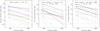 |
Fig. 12 Noise budget for the JVLA-C configuration as in Fig. 11. |
| In the text | |
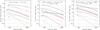 |
Fig. 13 Noise budget for the JVLA-B configuration as in Fig. 11. |
| In the text | |
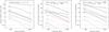 |
Fig. 14 Noise budget for the JVLA-A configuration as in Fig. 11. |
| In the text | |
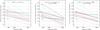 |
Fig. 15 Noise budget for the ATA telescope as in Fig. 11. |
| In the text | |
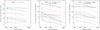 |
Fig. 16 Noise budget for the ASKAP telescope as in Fig. 11. |
| In the text | |
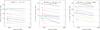 |
Fig. 17 Noise budget for the MeerKAT telescope as in Fig. 11. |
| In the text | |
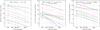 |
Fig. 18 Noise budget for the SKA1-Survey telescope as in Fig. 11. |
| In the text | |
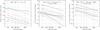 |
Fig. 19 Noise budget for the SKA1-Dish telescope as in Fig. 11. |
| In the text | |
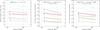 |
Fig. 20 Noise budget for the LOFAR High Band Core telescope as in Fig. 11. |
| In the text | |
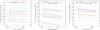 |
Fig. 21 Noise budget for the LOFAR High Band Remote telescope as in Fig. 11. |
| In the text | |
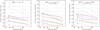 |
Fig. 22 Noise budget for the MWA telescope as in Fig. 11. |
| In the text | |
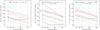 |
Fig. 23 Noise budget for the SKA1-Low Core telescope as in Fig. 11. |
| In the text | |
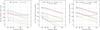 |
Fig. 24 Noise budget for the SKA1-Low extended telescope as in Fig. 11. |
| In the text | |
Current usage metrics show cumulative count of Article Views (full-text article views including HTML views, PDF and ePub downloads, according to the available data) and Abstracts Views on Vision4Press platform.
Data correspond to usage on the plateform after 2015. The current usage metrics is available 48-96 hours after online publication and is updated daily on week days.
Initial download of the metrics may take a while.