| Issue |
A&A
Volume 551, March 2013
|
|
|---|---|---|
| Article Number | A16 | |
| Number of page(s) | 8 | |
| Section | Interstellar and circumstellar matter | |
| DOI | https://doi.org/10.1051/0004-6361/201219805 | |
| Published online | 11 February 2013 | |
The Origem Loop
National Astronomical Observatories, Chinese Academy of
Sciences,
Jia-20 Datun Road, Chaoyang District,
100012
Beijing,
PR China
e-mail: This email address is being protected from spambots. You need JavaScript enabled to view it.
Received:
13
June
2012
Accepted:
6
December
2012
Abstract
Context. The Origem Loop in the Galactic anticentre was discovered in 1970s. It has been suggested that it is a large supernova remnant. One later argument is that it is a chance superposition of unrelated radio sources.
Aims. We attempt to understand the properties of the Origem Loop.
Methods. Available multi-frequency radio data were used to determine the radio spectra of different parts of the Origem Loop and the polarization properties of the loop.
Results. Newly available sensitive observations show that the Origem Loop is a loop of more than 6° in diameter. It consists of a large non-thermal arc in the north, which we call the Origem Arc, and several known thermal H II regions in the south. Polarized radio emission associated with the arc was detected at λ6 cm, revealing tangential magnetic fields. The arc has a brightness-temperature spectral index of β = −2.70, indicating its non-thermal nature as a supernova remnant. We estimate the distance to the Origem Arc to be about 1.7 kpc, similar to those of some H II regions in the southern part of the loop.
Conclusions. The Origem Loop is a visible loop in the sky, which consists of a supernova remnant arc in the north and H II regions in the south.
Key words: ISM: supernova remnants / radio continuum: ISM / ISM: individual objects: Origem Loop
© ESO, 2013
1. Introduction
Several giant loops were recognized in the early radio sky maps, i.e. Loop I (Hanbury Brown et al. 1960), Loop II (Large et al. 1962), Loop III (Quigley & Haslam 1965), and Loop IV (Large et al. 1966). By comparing the radio continuum, Hα, interstellar polarization and the H I observations of the four loops, Haslam et al. (1971) did a general review of these giant structures. Berkhuijsen et al. (1971) summarized the geometric parameters of the four loops, and proposed that they were produced by supernova explosions. Besides these four giant loops, there are also loops with smaller sizes, i.e. the Lupus Loop (Gardner & Milne 1965) and the Cygnus Loop (Walsh & Brown 1955), which have been definitely identified as supernova remnants (SNRs) and are collected in the well-known SNR catalogue compiled by Dave Green (Green 2009).
The Origem Loop is another known Galactic radio loop discovered in 1970s by Berkhuijsen (1974) on the 178 MHz radio map (Caswell & Crowther 1969) in the Galactic anticentre region between the constellations Orion and Gemini. However, its nature is under debate. It was first proposed that the loop is an old SNR at a distance of about 1 kpc with a diameter of about 5° (Berkhuijsen 1974), but it was later argued by Caswell (1985) that it is a possible projection effect of several unrelated H II regions, many extra-Galactic sources and a discrete small SNR G192.8−1.1 (PKS 0607+17) with a diameter of about 80′. However, Gao et al. (2011a) have disproved that G192.8−1.1 being an SNR. They find that it is a thermal emitter by using the Urumqi λ6 cm (Gao et al. 2010), the Effelsberg λ11 cm (Fürst et al. 1990), and the Effelsberg λ21 cm (Reich et al. 1997) survey data. Probably because of its large size, there were few follow-up observations of the Origem Loop after Berkhuijsen (1974). Caswell (1985) discussed the region of G192.8−1.1 and some nearby H II regions, but did not study the northern part of the Origem Loop. Krymkin & Sidorchuk (1988) made brightness temperature scans of nearly the entire loop with the UTR-2 and RATAN 600 radio telescopes at five frequencies, from 14.7 MHz to 3950 MHz. They claimed to have discovered a new feature, namely GR 0625+16, as another possible discrete SNR besides the “SNR” G192.8−1.1. However, the GR 0625+16 corresponds exactly to the northern arc of the Origem Loop.
Parameters of the survey data for the images of the Origem Loop.
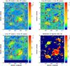 |
Fig. 1 From top left a), top right b)
to bottom left panel c): λ6 cm,
λ11 cm, and the λ21 cm total intensity images of
the Origem Loop. The angular resolutions are 9 |
High quality multi-frequency radio survey data with sufficient sensitivity and angular resolution are now available, which can be used to investigate the properties of the Origem Loop. We introduce in Sect. 2 the data sets we use, and present the analysis in Sect. 3. A summary is given in Sect. 4.
2. Data
The Origem Loop clearly shows up in the λ6 cm total intensity and
polarization images from the Sino-German λ6 cm polarization survey of the
Galactic plane1 (Gao
et al. 2010), which motivated us to seek a better understanding of this large
structure. Other public radio data are available from the Effelsberg λ11 cm
(2.7 GHz, Fürst et al. 1990) and
λ21 cm (1.4 GHz) Galactic plane survey (Reich et al. 1997), which can be downloaded from the survey sampler of the
Max-Planck-Institut für Radioastronomie (MPIfR)2, the
WMAP 7-year K-band (22.8 GHz, λ1.3 cm) survey data (Jarosik et al. 2011) retrieved from the website of
NASA3, the λ21 cm Effelsberg Medium
Latitude Survey (EMLS) data (Uyanıker et al. 1998,
1999), and the DRAO λ21 cm
polarization survey data (Wolleben et al. 2006), both
of which were also obtained from the survey sampler of MPIfR. In the following discussions,
we use the observing wavelength to indicate the data set. Specifically the
λ21 cm data stands for the Effelsberg Galactic plane survey data (Reich et al. 1997), unless special statements are made.
The angular resolution is 9 5 for the
λ6 cm image, 43 for
λ11 cm image, 94 for
λ21 cm image, 528 for
λ1.3 cm, 935 for EMLS
λ21 cm, and 36′ for DRAO λ21 cm images. Among them, the
λ6 cm and λ1.3 cm observations provided both total
intensity and polarization measurements, the DRAO λ21 cm data provided only
the polarization image, while the rest give only the total intensity maps. The Effelsberg
λ21 cm Galactic plane survey (Reich
et al. 1997) has a latitude limit of b = ± 4°. Therefore, we used
the EMLS data to fill the blank region above b = 4°, but we do not have any
data for the region below b = −4°. Basic parameters of these data sets
are summarized in Table 1. As done by Gao et al.
(2011b), the “background filtering” technique developed by Sofue & Reich (1979) was applied to λ6 cm,
λ11 cm, and λ21 cm images to separate the unrelated
large-scale Galactic diffuse emission from the Origem Loop emission. A twisted hyper plane
defined by the corner mean values of each image was subtracted to find the local zero level
around the Origem Loop. The final λ6 cm, λ11 cm,
λ21 cm total intensity images of the Origem Loop are shown in Fig. 1. The λ11 cm image was convolved to an
angular resolution of 95 to get a higher
signal-to-noise ratio.
5 for the
λ6 cm image, 43 for
λ11 cm image, 94 for
λ21 cm image, 528 for
λ1.3 cm, 935 for EMLS
λ21 cm, and 36′ for DRAO λ21 cm images. Among them, the
λ6 cm and λ1.3 cm observations provided both total
intensity and polarization measurements, the DRAO λ21 cm data provided only
the polarization image, while the rest give only the total intensity maps. The Effelsberg
λ21 cm Galactic plane survey (Reich
et al. 1997) has a latitude limit of b = ± 4°. Therefore, we used
the EMLS data to fill the blank region above b = 4°, but we do not have any
data for the region below b = −4°. Basic parameters of these data sets
are summarized in Table 1. As done by Gao et al.
(2011b), the “background filtering” technique developed by Sofue & Reich (1979) was applied to λ6 cm,
λ11 cm, and λ21 cm images to separate the unrelated
large-scale Galactic diffuse emission from the Origem Loop emission. A twisted hyper plane
defined by the corner mean values of each image was subtracted to find the local zero level
around the Origem Loop. The final λ6 cm, λ11 cm,
λ21 cm total intensity images of the Origem Loop are shown in Fig. 1. The λ11 cm image was convolved to an
angular resolution of 95 to get a higher
signal-to-noise ratio.
3. Results
Radio images in Fig. 1 at three different wavelengths
resemble each other in structures. At λ6 cm, the circle that indicates the
loop in Fig 1a has a radius of 200′ and is centred at
 . These values are different from
those of Berkhuijsen (1974), because we included the
region below δ = 14° (B1950), which was not included in the 178 MHz map
used by Berkhuijsen (1974). Our new sensitive
measurements enable us to detect fainter and more extended emission near the boundary of the
Origem Loop than ever before. The loop consists of four major parts: an elongated arc
structure extending from
. These values are different from
those of Berkhuijsen (1974), because we included the
region below δ = 14° (B1950), which was not included in the 178 MHz map
used by Berkhuijsen (1974). Our new sensitive
measurements enable us to detect fainter and more extended emission near the boundary of the
Origem Loop than ever before. The loop consists of four major parts: an elongated arc
structure extending from  to
to
 in the north, which can also be
recognized in the 178 MHz map shown by Berkhuijsen
(1974); the H II region BFS 52; and two complexes formed by several known
H II regions, i.e. SH 2-261, SH 2-254 to SH 2-258, the object G192.8−1.1 in the
south and southwest; and another group of H II regions SH 2-268, SH 2-270 in the
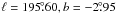
southeast. We marked the names of these known H II regions in Fig. 2.
in the north, which can also be
recognized in the 178 MHz map shown by Berkhuijsen
(1974); the H II region BFS 52; and two complexes formed by several known
H II regions, i.e. SH 2-261, SH 2-254 to SH 2-258, the object G192.8−1.1 in the
south and southwest; and another group of H II regions SH 2-268, SH 2-270 in the
southeast. We marked the names of these known H II regions in Fig. 2.
3.1. Spectral indices and their distribution
Spectral indices and their distribution are important properties for understanding the
nature of the extended radio sources. Shell-type SNRs usually have a brightness
temperature spectral index of β ~ −2.5
(Tb ~ νβ),
while the spectrum of an optically thin H II region is much flatter, normally
β ~ −2.1. We derived the brightness temperature spectral index
distribution of the Origem Loop (see Fig. 1d) using
the λ6 cm, λ11 cm, and the λ21 cm
images at an angular resolution of 95. A systematic
error of such a spectral index map comes from the uncertainties of the baselevel
determination due to the foreground/background subtraction. In Fig. 1d, the spectral index map shows reasonable thermal spectra for all
known H II regions, which demonstrates that the spectral map is reliable. The
northern arc of the Origem Loop, which we call the Origem Arc, obviously has a non-thermal
brightness temperature spectral index around β ~ −2.7 (flux density
spectral index α = β + 2 = −0.7). This region was once
singled out by Krymkin & Sidorchuk (1988)
in their brightness temperature scans and designated as GR 0625+16. They suggested that
GR 0625+16 is a discrete SNR with an integrated radio spectral index of
α = −0.48 ± 0.05. Although this spectral index is larger than the one
we derived from our new data, both indicate the non-thermal nature of the Origem Arc.
The TT-plot method (Turtle et al. 1962) was used
to verify the spectrum (see Fig. 3). The background
point sources were subtracted first, as in Gao et al.
(2011b). All images were then smoothed to a common angular resolution of
95. For the
entire Origem Arc spanning to
as indicated in Fig. 2, we obtained the spectral index of
β6−11 = −2.43 ± 1.23 from all the data pixels of
λ6 cm and λ11 cm, and
β6−21 = −2.70 ± 0.28 for λ6 cm and
λ21 cm. Although the temperature measurements for each pixel are not
independent, the TT-plots give the correct brightness temperature spectral indices and the
uncertainty estimates, as we tested by using the independent pixels. The TT-plot of the
brighter part (high signal-to-noise ratio) of the arc
( ) gives consistent results as
β6−11 = −2.45 ± 1.06, and
β6−21 = −2.65 ± 0.29. All these spectral values agree
well with the spectral index map shown in Fig. 1d.
) gives consistent results as
β6−11 = −2.45 ± 1.06, and
β6−21 = −2.65 ± 0.29. All these spectral values agree
well with the spectral index map shown in Fig. 1d.
The other parts of the Origem Loop have different properties. The well-known
H II region, BFS 52 (Blitz et al. 1982),
has the central coordinates of  , and the quasar
J061357.6+130645 (Aslan et al. 2010) is located at
, and the quasar
J061357.6+130645 (Aslan et al. 2010) is located at
 . Both have a flat spectrum
(β ~ −2.1). A circular region located at
. Both have a flat spectrum
(β ~ −2.1). A circular region located at
 with a diameter of 1° was
found to be very interesting. It has a brightness temperature spectral index of about
β ~ −2.5 according to Fig. 1d.
The TT-plot of this region gives a consistent result of
β6−21 = −2.33 ± 0.23, but this also implies a
possibility of being a flat-spectrum thermal emission. We assign its name G195.60−2.95
and mark it using a circle with a central “N” in Figs. 2 and 4. It has strong Hα emission and ring-shaped dust
emission (see Figs. 4 and 7). The high ratio between
the 60 μm infrared and the λ6 cm continuum emission
(~1400) indicates it as a probable thermal H II region. G192.8−1.1 has a flat
thermal spectrum and is not an SNR, as discussed in Gao
et al. (2011a).
with a diameter of 1° was
found to be very interesting. It has a brightness temperature spectral index of about
β ~ −2.5 according to Fig. 1d.
The TT-plot of this region gives a consistent result of
β6−21 = −2.33 ± 0.23, but this also implies a
possibility of being a flat-spectrum thermal emission. We assign its name G195.60−2.95
and mark it using a circle with a central “N” in Figs. 2 and 4. It has strong Hα emission and ring-shaped dust
emission (see Figs. 4 and 7). The high ratio between
the 60 μm infrared and the λ6 cm continuum emission
(~1400) indicates it as a probable thermal H II region. G192.8−1.1 has a flat
thermal spectrum and is not an SNR, as discussed in Gao
et al. (2011a).
The TT-plot can be used to reveal different emitting components with different spectral indices (e.g. Xiao et al. 2008). The TT-plot of the southern half of the Origem Loop shows that thermal emission is overwhelmingly dominant. Unlike in the northern arc, no evidence was found for any detectable unambiguous non-thermal emission component in the south (see Fig. 5).
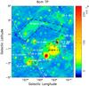 |
Fig. 2 λ6 cm total intensity image with the prominent H II regions marked with “ + ” and labelled with the names. The disproved SNR, G192.8−1.1, was also marked with a circle of the pink dashed line. The outer red dotted line delineates the common area of the observations by Krymkin & Sidorchuk (1988) and our image, while the red dashed line indicates the field shown in Caswell (1985). The white dashed-dot line shows the declination of δ = 14° (Epoch 1950). The region on the left side of this line was not included in the 178 MHz map used by Berkhuijsen (1974). The area outlined by the black dashed line, containing the Origem Arc, was used for the TT-plot in Sect. 3.1. A probable new H II region G195.60-2.95 is marked using a circle with the letter “N” inside. |
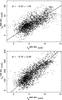 |
Fig. 3 TT-plot for all the pixels in the Origem Arc region (outlined by the black dashed line in Fig. 2) between λ6 cm and λ11 cm (upper panel) and between λ6 cm and λ21 cm (bottom panel). |
3.2. Polarization
Observations of polarized emission at λ6 cm, λ1.3 cm,
and DRAO λ21 cm were available for the Origem Loop region. However, only
the λ6 cm data show the weak polarized emission associated with the
Origem Arc (see the left panel of Fig. 4), in addition to the diffuse polarized background emission in the lower part
of the map. At λ6 cm, the polarized emission is clearly detected within
the arc even at the western end where the total intensity becomes very weak. The
polarization fraction is about 40% on average. The polarization B-field vectors
(E + 90°) are found to follow the arc, indicating the
presence of tangential magnetic fields. We also noticed that the depolarization zones seen
at λ6 cm are correlated with the enhanced Hα emission
(see the right panel of Fig. 4),
e.g. the area around  , probably due to the
Faraday rotation caused by the magnetic fields and the thermal electrons. A shuttle-shaped
depolarization zone is found to cross the Origem Arc from northwest to southeast, where
bright Hα filaments have good positional correspondences and
morphological similarities.
, probably due to the
Faraday rotation caused by the magnetic fields and the thermal electrons. A shuttle-shaped
depolarization zone is found to cross the Origem Arc from northwest to southeast, where
bright Hα filaments have good positional correspondences and
morphological similarities.
In the southern part of the Origem Loop region, a few large polarization patches were
detected within and outside the loop. However, none of them seems to be related either to
the Origem Loop or G192.8−1.1 (Gao et al. 2011a).
No arc-shaped structure in polarization can be found. In the area of
 , the H II region
SH 2-261 acts as a Faraday screen.
, the H II region
SH 2-261 acts as a Faraday screen.
At λ1.3 cm, no polarized emission is visible in the entire area of the Origem Loop. Using the average brightness temperature of the polarized emission in the arc at λ6 cm, 5.0 mK Tb, and the spectral index of β = −2.70, we estimated the brightness temperature of the polarized emission of the arc at λ1.3 cm to be about 0.07 mK Tb. It is about the same level as the noise in the K-band data, which could account for the non-detection of polarization.
At λ21 cm, no correlated polarized emission was detected in the Origem Arc from the DRAO data, either. The beam size of the DRAO data is 36′. Beam and depth depolarization could diminish any polarized emission. The non-detection might also imply a very near polarization horizon at λ21 cm in this direction.
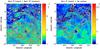 |
Fig. 4 left panel: λ6 cm polarization image
(9 |
3.3. Distances of the Origem Arc and H II regions
Distance of the known H II regions.
The observed tangential magnetic fields within the Origem Arc and the non-thermal spectrum are key evidence for identifying it as an SNR. To verify that this SNR and the H II regions located in the southern part of the Origem Loop are physically related, we need to know their distances first.
Despite the large uncertainty, the empirical relation between surface brightness and
diameter (Σ-D) of SNRs provides distance estimates of shell-type SNRs in case no related
H I or molecular clouds (MC) are associated with the SNR. For the entire Origem
Arc, a sector with an opening angle of 128°, the flux density at λ6 cm is
measured to be S6 cm = 8.5 ± 0.9 Jy after subtracting the
background sources. We extrapolate S6 cm to the flux density
at 1 GHz with the spectral index of α = −0.7. Using the arc radius of
3 3 measured on
the map, we obtained a radio surface brightness of the Origem Arc of
Σ1 GHz = (8.6 ± 0.9) × 10-23 Wm-2 Hz-1 sr-1.
According to the Σ-D relation found by Case &
Bhattacharya (1998), the diameter of the Origem Loop is estimated to be about
195 pc and the distance to be about 1.7 kpc. As emphasized by Case & Bhattacharya (1998), the deviation of an individual
estimate derived from their work can be as large as 40%, which puts the Origem Arc within
a distance range between 1.0 and 2.4 kpc. Asvarov
(2006) built a model that describes the evolution of the surface brightness and
the diameter of shell-type SNRs with time. From his Σ-D relation (see his Fig. 6), we
estimated that the Origem Arc has a diameter between 100 and 300 pc, corresponding to a
distance range of 0.9 to 2.6 kpc. We therefore conclude that the Origem Arc is likely to
have a distance of 1.7 ± 0.8 kpc.
3 measured on
the map, we obtained a radio surface brightness of the Origem Arc of
Σ1 GHz = (8.6 ± 0.9) × 10-23 Wm-2 Hz-1 sr-1.
According to the Σ-D relation found by Case &
Bhattacharya (1998), the diameter of the Origem Loop is estimated to be about
195 pc and the distance to be about 1.7 kpc. As emphasized by Case & Bhattacharya (1998), the deviation of an individual
estimate derived from their work can be as large as 40%, which puts the Origem Arc within
a distance range between 1.0 and 2.4 kpc. Asvarov
(2006) built a model that describes the evolution of the surface brightness and
the diameter of shell-type SNRs with time. From his Σ-D relation (see his Fig. 6), we
estimated that the Origem Arc has a diameter between 100 and 300 pc, corresponding to a
distance range of 0.9 to 2.6 kpc. We therefore conclude that the Origem Arc is likely to
have a distance of 1.7 ± 0.8 kpc.
The average kinematic distance of several H II regions located in the southern part of the Origem Loop was found to be 1.2 ± 0.7 kpc (Berkhuijsen 1974). However, as noted by Caswell (1985), the kinematic distances have large uncertainties. More accurate distance determinations towards these H II regions have been obtained through the photometric and trigonometric parallax measurements as we listed in Table 2, except for SH 2-270. The lower half of the Origem Loop consists of the H II regions BFS 52, SH 2-254 to 258, SH 2-261, SH 2-268, and the H II region SH 2-266, which have similar distances to the Origem Arc, and the other distant H II regions SH 2-253, SH 2-267, SH 2-269, SH 2-271, and SH 2-272. We could not get the distances of the object G192.8−1.1 and the newly identified object G195.60−2.95.
3.4. Signatures at other wavelengths
Berkhuijsen (1974) searched for possible H I structures associated with the Origem Loop, however, no clue was found. Denoyer et al. (1977) proposed that an H I jet, which appears at ℓ ~ 197°, b ~ 2° may be related to the Origem Arc, although the jet is extended beyond its boundary. This jet is a part of the prominent H I structure, the anticentre shell (ACS), which was discovered by Heiles (1984). We checked the new H I data from the Leiden/Argentina/Bonn H I survey (Hartmann & Burton 1997; Kalberla et al. 2005) and the GALFA H I DR1 data4 for a much larger area (20° × 20°). We found that the ACS is prominent in the negative velocity map and disappears in the positive velocity map. This clearly differs from the positive CO radial velecity associated with the H II regions discussed above. Moreover, the ACS has a much larger size (~30° in diameter) than the Origem Loop. For the velocity 0.0 to 32.5 km s-1, no associated H I structure is found around the Origem Loop.
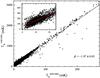 |
Fig. 5 TT-plot for the southern part of the Origem Loop between λ6 cm and
λ21 cm. The inner small image is the zoom-in picture for the
value |

Berkhuijsen (1974) investigated the relation between the Origem Loop and the H II regions. Based on the age of the loop and the evolution timecale from protostars to the H II regions, it was hard to tell whether the Origem Loop triggered the star formation that leads to the H II regions in the south. Using the physical size determined in this work, adopting Eq. (3) in Berkhuijsen (1974), the Origem Arc is about 1 to 3 Myr old. Chavarría et al. (2008) estimated the ages of the H II regions SH 2-254 to 258 from an expansion model of a Strömgren sphere, ranging between 0.1 Myr to 5.0 Myr. Bieging et al. (2009) have proposed a sequential star formation scenario from interaction between the H II regions and molecular clouds, which indicates that at least the younger H II regions SH 2-255 to 257 were triggered by SH 2-254.
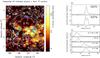 |
Fig. 6 Left panel: CO intensity map integrated from 0.0 to 32.5 km s-1, overlaid by the λ6 cm total intensity contours as shown in Fig. 1. Each pixel value was normalized by dividing by the maximum integrated intensity in the image. The green crosses represent the proto-stellar candidates selected from the IRAS point source catalogue by the criteria introduced by Junkes et al. (1992), while the blue-white triangles are the massive young stellar objects found in the Red MSX survey. Top right panel: normalized CO emission profile for the two areas marked with the black “plus” in the left panel. Bottom right panel: CO spectra for the H II regions SH 2-254 to 258, BFS 52, SH 2-253, and SH 2-269. The brightness temperature in each region was also normalized. |
The interaction between the SNR shock and the ambient molecular clouds should broaden the linewidth. For example, IC 443, a famous SNR-MC interaction case, clearly shows a high CO J = 3−2/CO J = 2−1 ratio and the broadening of CO emission lines (Zhang et al. 2010; Xu et al. 2011). Broadened CO J = 1−0 lines were also detected in another SNR-MC interaction case (Byun et al. 2006). Public CO J = 3−2 and CO J = 2−1 data covering the Origem Loop region are not available. We checked the CO J = 1−0 data of the Origem Loop region from the CO survey5 (Dame et al. 2001). The radial velocities of the CO emission peaks associated with these H II regions were previously measured and given by Blitz et al. (1982), as we listed in our Table 2. Therefore, we integrated the CO emission in the velocity range from 0.0 km s-1 to 32.5 km s-1 and show the result in the left-hand panel of Fig. 6. We find that the most intense CO emission comes from the area of G192.8−1.1. It has a roughly similar morphology to the λ6 cm continuum emission as illustrated by the contour lines in Fig. 6. An obvious gap of CO emission is seen at the edge of the continuum emission in the southwest of G192.8−1.1. We checked the velocity-intensity relation at two positions indicated by “plus” in the left-hand panel of Fig. 6 and also the velocity-intensity plots for the H II region SH 2-254 to SH 2-258, BFS 52 for the possible interaction group and the H II regions SH 2-253, SH 2-269 for the non-interaction group. As shown in the right-hand panel of Fig. 6, all of the radial velocities corresponding to the peak CO emission for the H II regions are consistent with those found by Blitz et al. (1982). We checked the linewidths for several hundred non-interacting H II regions (Anderson et al. 2009; Russeil & Castets 2004) and found the average values are in the range of 3 ~ 6 km s-1. SH 2-254 to 258, BFS 52, SH 2-253, and SH 2-269 have similar linewidths, and no significant rise in the line wings can be seen. Therefore there are no hints for the interaction between SNR and clouds for H II region formation.
We searched for massive young stellar objects (YSOs) in the Origem Loop region from the Red MSX Source Survey database6 and for the protostellar candidates in the IRAS point source catalogue. They are marked in Fig. 6. Several of them are coincident and most of them are located in the regions where CO emission is prominent. The YSOs in the Origem Loop region do not show over density on the northern Origem Arc or on the shell-like structure where the continuum-CO boundary exists.
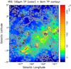 |
Fig. 7 100 μm dust map (2′ resolution) overlaid with the contours of the λ6 cm total intensity. The contours are the same as in Fig. 1. |
Infrared (dust) image was also checked by Berkhuijsen (1974), nothing coincided with the Origem Arc (see her Fig. 3). From the IRIS 100 μm dust image (Miville-Deschênes & Lagache 2005) of the Origem Loop region shown in Fig. 7, we found that the dust emission is well correlated with the H II regions in the south. The two interacting H II regions SH 2-255 and SH 2-257 triggered star formation in between them (Ojha et al. 2011). A large number of YSOs were identified on their boundary. The object G195.60-2.95 has an incomplete ring structure, and the infrared emission gets enhanced between it and the known H II regions SH 2-268, which is about 1.3 kpc away. However, we do not get any YSOs on the intensive infrared emission zone. This might be due to limitation of the infrared data sets we use. The apparent sizes of the infrared bubbles in the inner Galaxy are generally smaller than the one around G195.60−2.95 (Simpson et al. 2012), which may imply a small distance to G195.60−2.95. An infrared loop was also found around the SNR (Koo et al. 2008). However, the polarization measurement at λ6 cm and the infrared/radio ratio of G195.60-2.95 strongly suggest that it is an H II region.
We checked the 0.1–0.4 keV and 0.4–2.4 keV ROSAT X-ray images7, and no associated structure with the Origem Loop was found.
4. Summary
We used multi-frequency survey data to revisit the Origem Loop in the anticentre of the Galaxy. The Origem Arc is a polarized non-thermal emission structure with a spectral index of β = −2.70, indicating that it is a shell-type SNR. We estimated its distance to be 1.7 ± 0.8 kpc.
Using the new radio data, we discussed the possibilities of a physical association between the SNR and the H II regions located in the south of the Origem Loop. The TT-plots for different emission components, the width of CO lines, and age estimates did not show any evidence of a non-thermal southern arc or the interaction between the SNR and the H II regions in the south. Associated infrared emission is seen to be closely related to the H II regions in the southern part of the loop. No H I or X-ray emission correlated with the Origem Loop was found.
Acknowledgments
We would like to thank the referee, Dr. Elly Berkhuijsen, for constructive and helpful comments. The Sino-German λ6 cm polarization survey was carried out with a receiver system constructed by Mr. Otmar Lochner at MPIfR mounted at the Nanshan 25-m telescope of the Urumqi Observatory of NAOC. The MPG and the NAOC/CAS supported the construction of the receiving system by special funds. We thank Mr. Maozheng Chen and Mr. Jun Ma for qualified maintenance of the receiving system for many years. The authors are supported by the National Natural Science foundation of China (10833003) and the Partner group of the MPIfR at NAOC in the framework of the exchange program between MPG and CAS for many bilateral visits. X.Y.G. is additionally supported by the Young Researcher Grant of National Astronomical Observatories, Chinese Academy of Sciences. This paper made use of information from the Red MSX Source survey database at www.ast.leeds.ac.uk/RMS, which was constructed with support from the Science and Technology Facilities Council of the UK. This paper also utilizes data from Galactic ALFA HI (GALFA HI) survey data set obtained with the Arecibo L-band Feed Array (ALFA) on the Arecibo 305 m telescope. Arecibo Observatory is part of the National Astronomy and Ionosphere Center, which is operated by Cornell University under Cooperative Agreement with the US National Science Foundation. The GALFA HI surveys are funded by the NSF through grants to Columbia University, the University of Wisconsin, and the University of California.
References
- Anderson, L. D., Bania, T. M., Jackson, J. M., et al. 2009, ApJS, 181, 255 [NASA ADS] [CrossRef] [Google Scholar]
- Aslan, Z., Gumerov, R., Jin, W., et al. 2010, A&A, 510, A10 [NASA ADS] [CrossRef] [EDP Sciences] [Google Scholar]
- Asvarov, A. I. 2006, A&A, 459, 519 [NASA ADS] [CrossRef] [EDP Sciences] [Google Scholar]
- Berkhuijsen, E. M. 1974, A&A, 35, 429 [NASA ADS] [Google Scholar]
- Berkhuijsen, E. M., Haslam, C. G. T., & Salter, C. J. 1971, A&A, 14, 252 [NASA ADS] [Google Scholar]
- Bieging, J. H., Peters, W. L., Vi la Vilaro, B., Schlottman, K., & Kulesa, C. 2009, AJ, 138, 975 [NASA ADS] [CrossRef] [Google Scholar]
- Blitz, L., Fich, M., & Stark, A. A. 1982, ApJS, 49, 183 [NASA ADS] [CrossRef] [Google Scholar]
- Byun, D.-Y., Koo, B.-C., Tatematsu, K., & Sunada, K. 2006, ApJ, 637, 283 [NASA ADS] [CrossRef] [Google Scholar]
- Case, G. L., & Bhattacharya, D. 1998, ApJ, 504, 761 [Google Scholar]
- Caswell, J. L. 1985, AJ, 90, 1076 [NASA ADS] [CrossRef] [Google Scholar]
- Caswell, J. L., & Crowther, J. H. 1969, MNRAS, 145, 181 [NASA ADS] [Google Scholar]
- Chavarría, L. A., Allen, L. E., Hora, J. L., Brunt, C. M., & Fazio, G. G. 2008, ApJ, 682, 445 [NASA ADS] [CrossRef] [Google Scholar]
- Dame, T. M., Hartmann, D., & Thaddeus, P. 2001, ApJ, 547, 792 [NASA ADS] [CrossRef] [Google Scholar]
- Denoyer, L. K., Button, L., Chaffin, D., & Nieznanski, J. 1977, ApJ, 213, 379 [NASA ADS] [CrossRef] [Google Scholar]
- Fürst, E., Reich, W., Reich, P., & Reif, K. 1990, A&AS, 85, 691 [NASA ADS] [Google Scholar]
- Gao, X. Y., Reich, W., Han, J. L., et al. 2010, A&A, 515, A64 [NASA ADS] [CrossRef] [EDP Sciences] [Google Scholar]
- Gao, X. Y., Han, J. L., Reich, W., et al. 2011a, A&A, 529, A159 [NASA ADS] [CrossRef] [EDP Sciences] [Google Scholar]
- Gao, X. Y., Sun, X. H., Han, J. L., et al. 2011b, A&A, 532, A144 [NASA ADS] [CrossRef] [EDP Sciences] [Google Scholar]
- Gardner, F. F., & Milne, D. K. 1965, AJ, 70, 754 [NASA ADS] [CrossRef] [Google Scholar]
- Green, D. A. 2009, Bull. Astron. Soc. India, 37, 45 [Google Scholar]
- Hanbury Brown, R., Davies, R. D., & Hazard, C. 1960, The Observatory, 80, 191 [NASA ADS] [Google Scholar]
- Hartmann, D., & Burton, W. B. 1997, Atlas of Galactic Neutral Hydrogen, eds. D. Hartmann, & W. B. Burton [Google Scholar]
- Haslam, C. G. T., Kahn, F. D., & Meaburn, J. 1971, A&A, 12, 388 [NASA ADS] [Google Scholar]
- Heiles, C. 1984, ApJS, 55, 585 [NASA ADS] [CrossRef] [Google Scholar]
- Honma, M., Bushimata, T., Choi, Y. K., et al. 2007, PASJ, 59, 889 [NASA ADS] [Google Scholar]
- Jarosik, N., Bennett, C. L., Dunkley, J., et al. 2011, ApJS, 192, 14 [NASA ADS] [CrossRef] [Google Scholar]
- Junkes, N., Fuerst, E., & Reich, W. 1992, A&A, 261, 289 [NASA ADS] [Google Scholar]
- Kalberla, P. M. W., Burton, W. B., Hartmann, D., et al. 2005, A&A, 440, 775 [NASA ADS] [CrossRef] [EDP Sciences] [Google Scholar]
- Koo, B.-C., McKee, C. F., Lee, J.-J., et al. 2008, ApJ, 673, L147 [NASA ADS] [CrossRef] [Google Scholar]
- Krymkin, V. V., & Sidorchuk, M. A. 1988, A&A, 200, 185 [NASA ADS] [Google Scholar]
- Lahulla, J. F. 1987, AJ, 94, 1062 [NASA ADS] [CrossRef] [Google Scholar]
- Large, M. I., Quigley, M. J. S., & Haslam, C. G. T. 1962, MNRAS, 124, 405 [NASA ADS] [Google Scholar]
- Large, M. I., Quigley, M. F. S., & Haslam, C. G. T. 1966, MNRAS, 131, 335 [NASA ADS] [CrossRef] [Google Scholar]
- Miville-Deschênes, M., & Lagache, G. 2005, ApJS, 157, 302 [NASA ADS] [CrossRef] [Google Scholar]
- Ojha, D. K., Samal, M. R., Pandey, A. K., et al. 2011, ApJ, 738, 156 [NASA ADS] [CrossRef] [Google Scholar]
- Quigley, M. J. S., & Haslam, C. G. T. 1965, Nature, 208, 741 [NASA ADS] [CrossRef] [Google Scholar]
- Reich, P., Reich, W., & Fürst, E. 1997, A&AS, 126, 413 [NASA ADS] [CrossRef] [EDP Sciences] [Google Scholar]
- Reid, M. J., Menten, K. M., Brunthaler, A., et al. 2009, ApJ, 693, 397 [NASA ADS] [CrossRef] [Google Scholar]
- Russeil, D. 2003, A&A, 397, 133 [NASA ADS] [CrossRef] [EDP Sciences] [Google Scholar]
- Russeil, D., & Castets, A. 2004, A&A, 417, 107 [NASA ADS] [CrossRef] [EDP Sciences] [Google Scholar]
- Rygl, K. L. J., Brunthaler, A., Reid, M. J., et al. 2010, A&A, 511, A2 [NASA ADS] [CrossRef] [EDP Sciences] [Google Scholar]
- Simpson, R. J., Povich, M. S., Kendrew, S., et al. 2012, MNRAS, 424, 2442 [NASA ADS] [CrossRef] [Google Scholar]
- Sofue, Y., & Reich, W. 1979, A&AS, 38, 251 [NASA ADS] [Google Scholar]
- Turtle, A. J., Pugh, J. F., Kenderdine, S., & Pauliny-Toth, I. I. K. 1962, MNRAS, 124, 297 [NASA ADS] [CrossRef] [Google Scholar]
- Uyanıker, B., Fürst, E., Reich, W., Reich, P., & Wielebinski, R. 1998, A&AS, 132, 401 [NASA ADS] [CrossRef] [EDP Sciences] [Google Scholar]
- Uyanıker, B., Fürst, E., Reich, W., Reich, P., & Wielebinski, R. 1999, A&AS, 138, 31 [NASA ADS] [CrossRef] [EDP Sciences] [Google Scholar]
- Walsh, D., & Brown, R. H. 1955, Nature, 175, 808 [NASA ADS] [CrossRef] [Google Scholar]
- Wolleben, M., Landecker, T. L., Reich, W., & Wielebinski, R. 2006, A&A, 448, 411 [NASA ADS] [CrossRef] [EDP Sciences] [Google Scholar]
- Xiao, L., Fürst, E., Reich, W., & Han, J. L. 2008, A&A, 482, 783 [NASA ADS] [CrossRef] [EDP Sciences] [Google Scholar]
- Xu, J.-L., Wang, J.-J., & Miller, M. 2011, ApJ, 727, 81 [NASA ADS] [CrossRef] [Google Scholar]
- Zhang, Z., Gao, Y., & Wang, J. 2010, Sci. China G: Phys. Astron., 53, 1357 [NASA ADS] [CrossRef] [Google Scholar]
All Tables
All Figures
|
Fig. 1 From top left a), top right b)
to bottom left panel c): λ6 cm,
λ11 cm, and the λ21 cm total intensity images of
the Origem Loop. The angular resolutions are 9 |
| In the text | |
|
Fig. 2 λ6 cm total intensity image with the prominent H II regions marked with “ + ” and labelled with the names. The disproved SNR, G192.8−1.1, was also marked with a circle of the pink dashed line. The outer red dotted line delineates the common area of the observations by Krymkin & Sidorchuk (1988) and our image, while the red dashed line indicates the field shown in Caswell (1985). The white dashed-dot line shows the declination of δ = 14° (Epoch 1950). The region on the left side of this line was not included in the 178 MHz map used by Berkhuijsen (1974). The area outlined by the black dashed line, containing the Origem Arc, was used for the TT-plot in Sect. 3.1. A probable new H II region G195.60-2.95 is marked using a circle with the letter “N” inside. |
| In the text | |
|
Fig. 3 TT-plot for all the pixels in the Origem Arc region (outlined by the black dashed line in Fig. 2) between λ6 cm and λ11 cm (upper panel) and between λ6 cm and λ21 cm (bottom panel). |
| In the text | |
|
Fig. 4 left panel: λ6 cm polarization image
(9 |
| In the text | |
|
Fig. 5 TT-plot for the southern part of the Origem Loop between λ6 cm and
λ21 cm. The inner small image is the zoom-in picture for the
value |
| In the text | |
|
Fig. 6 Left panel: CO intensity map integrated from 0.0 to 32.5 km s-1, overlaid by the λ6 cm total intensity contours as shown in Fig. 1. Each pixel value was normalized by dividing by the maximum integrated intensity in the image. The green crosses represent the proto-stellar candidates selected from the IRAS point source catalogue by the criteria introduced by Junkes et al. (1992), while the blue-white triangles are the massive young stellar objects found in the Red MSX survey. Top right panel: normalized CO emission profile for the two areas marked with the black “plus” in the left panel. Bottom right panel: CO spectra for the H II regions SH 2-254 to 258, BFS 52, SH 2-253, and SH 2-269. The brightness temperature in each region was also normalized. |
| In the text | |
|
Fig. 7 100 μm dust map (2′ resolution) overlaid with the contours of the λ6 cm total intensity. The contours are the same as in Fig. 1. |
| In the text | |
Current usage metrics show cumulative count of Article Views (full-text article views including HTML views, PDF and ePub downloads, according to the available data) and Abstracts Views on Vision4Press platform.
Data correspond to usage on the plateform after 2015. The current usage metrics is available 48-96 hours after online publication and is updated daily on week days.
Initial download of the metrics may take a while.