| Issue |
A&A
Volume 550, February 2013
|
|
|---|---|---|
| Article Number | A2 | |
| Number of page(s) | 7 | |
| Section | Stellar structure and evolution | |
| DOI | https://doi.org/10.1051/0004-6361/201220388 | |
| Published online | 15 January 2013 | |
HD 165246: an early-type binary with a low mass ratio⋆
1 Astronomical Institute of the Charles University, Faculty of Mathematics and Physics, V Holešovičkách 2, 180 00 Praha 8, Czech Republic
e-mail: This email address is being protected from spambots. You need JavaScript enabled to view it.
2 Department of Physics, Faculty of Science, University of Zagreb, Bijenička cesta 32, 10 000 Zagreb, Croatia
Received: 14 September 2012
Accepted: 27 November 2012
Abstract
Analyses of 13 FEROS spectra from the ESO archive and 617 V-band photometric observations from the ASAS3 database allowed us to demonstrate that HD 165246 is a double-lined spectroscopic binary. As an earlier finding revealed, HD 165246 is also an eclipsing system. We were able to derive consistent orbital and light-curve solutions and all basic physical properties of the system. The period of this O8 V + B7 V binary is 4 592706 and the semiamplitudes of the radial-velocity curves are K1 = 55.5 km s-1 and K2 = 321 km s-1. As the mass ratio is small (0.173), the secondary lines cannot be seen directly in the spectra; however the application of spectral disentangling allowed us to detect weak Balmer and He i lines of the secondary component. The primary component rotates with a high projected velocity of v sin i = 243 km s-1. A combined radial-velocity and light-curve solution led to the component masses and radii expected for the young stars of the given spectral types. Due to the high rotation velocity, the primary component might display changes in surface abundances of some elements. However, we did not find any significant differences with respect to the abundances of slowly rotating stars.
Key words: stars: early-type / binaries: eclipsing / stars: individual: HD 165246
Based on the spectra obtained with the European Southern Observatory telescopes and extracted from the ESO/ST-ECF Science Archive Facility, as well as on the V photometry from the ASAS3 archive.
© ESO, 2013
1. Introduction
Massive stars of spectral type O are astrophysically important in several aspects. Their evolution is fast and they affect the chemical composition of the circumstellar matter. Their accurate modelling via stellar-evolutionary models has to take into account a significant mass loss from these stars via stellar wind, a problem that has not yet been self-consistently solved. The most accurate way to obtain reliable physical properties of O stars is to study detached eclipsing binaries among them, though rare they are. Another problem of general importance is the formation of such massive stars. It was recently discussed by Chini et al. (2012), who found from their survey that the majority of known O stars form close binary systems with components of similar masses. The ratio of masses of binary components q = m2/m1 is a very important parameter; different theories of binary origin predict different mass ratio distributions. There might be an observational bias, however. Since O stars have very high luminosities, it is very hard to discover O-type binaries with a low mass ratio as the luminosity of the lighter component represents usually only a small fraction of the total luminosity of the system. In an earlier search, Garmany et al. (1980) found no case with q < 0.3 among the early-type binaries. Nowadays, a few binaries with q < 0.3 are known. Our literature survey revealed three massive binaries with (mutually similar) q of about 0.24:
-
O 5 star HD 37022 (θ 1 Ori C); see Kraus et al. (2009),
-
B7 Iab star HD 53975 (HR 2679); see Gies et al. (1994), and
-
O6 V star HD 199579 (HR 8023); see Williams et al. (2001).
Here, we shall report the discovery that the O8 V binary HD 165246 has an even lower mass ratio and is therefore worth investigating in detail.
2. Current knowledge about HD 165246
The star HD 165246 (CD − 24°13880; V = 7.7) was classified O8 V(n) by Walborn (1972). It is a visual binary ADS 11049 (WDS 18061-2412, separation 1 9, magnitude difference 4
 0) and a member of the O-type association Sgr OB1. There are several other binaries in this association: the eclipsing binaries V3903 Sgr (Vaz et al. 1997) and μ Sgr (Polidan & Plavec 1984), as well as the spectroscopic binaries HD 164402 (Stickland & Lloyd 1999), HD 164816 (Trepl et al. 2012), HD 165052 (Linder et al. 2007), and Herschel 36 (Arias et al. 2010). Otero (2007) discovered the eclipsing-binary nature of HD 165246 using the ASAS3 data (Pojmanski 2002) and derived a linear ephemeris
  (1)The minima are quite narrow, with the depths of 0m.10 and 0m.02 in the V band.
RVs of six strong spectral lines of the primary of HD 165246 measured on the FEROS spectra in SPEFO.
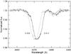 |
Fig. 1 Line profiles of the He i λ4471 line at phases close to quadratures. |
3. Spectroscopy and preliminary orbital solutions
In the ESO archive, there are 13 FEROS spectra taken by several observers in the years 2006 to 2009. The FEROS spectrograph works at the 2.2 m ESO/MPI telescope at La Silla. The spectra have a resolving power of 48 000 and cover the spectral region from 3575 to 9215 Å. They are available as pipeline products from the archive and are listed in Table 1. An example of the line profiles is in Fig. 1. There are also three spectra of this binary in the HST-STIS archive. They cover the wavelengths from 1160 to 1360 Å. However, due to short spectrograph echelle orders and the wide lines of the O8 star, the radial velocities (RVs), which we tried to determine from them, turned out unreliable and are not used here.
The FEROS spectra agree perfectly with the O8 V classification. We first measured the RVs using several He i lines (λλ4026 and 4471), He ii lines (λλ4541 and 4686), and Balmer Hβ and Hγ with the programme SPEFO (Horn et al. 1996; Škoda 1996), comparing the direct and flipped line profiles on the computer screen. The measured RVs are in Table 1.
The lines are quite wide, the projected rotation velocity being v sin i = 243 km s-1 (see later). The period and the conjunction time of the RV curve agree well with Otero’s ephemeris (Eq. (1)). The parameters of the RV curve can be determined with good accuracy. However, the small RV amplitude in the eclipsing binary is rather surprising: in the He ii lines λ4541 and λ4686, it is only ≈ 56 km s-1. No indications of the secondary lines are visible in the spectra (see lower panel in Fig. 3). Although the number of spectra is small and the photometry has only a modest signal-to-noise ratio (S/N), the phase distribution of the spectra is good and the orbit is well defined. To check whether a small orbital eccentricity is present, we derived trial orbital solutions using the programme SPEL1. This programme carries out automatically the test on the statistical significance of the orbital eccentricity suggested by Lucy & Sweeney (1971). The orbital solutions are summarized in Table 2. We note that the most reliably measurable lines all indicate a small, but significant orbital eccentricity. It is also seen that both the semiamplitudes and the systemic velocities differ from line to line. While the differences in the systemic velocities can be explained by the line blending of rotationally broadened lines, the differences in the semiamplitudes could be indicative of the presence of weak lines of the secondary. For that reason we prefer estimating the mass function from the mean semiamplitude of the He ii λ4541 and λ4686 lines, which should be only present in the spectrum of the primary. To this end, we used the mean RVs of both lines to derive another solution, also listed at the end of Table 2. It gives K1 = 55.9 ± 1.0 km s-1, therefore a low mass function of f(m) = 0.0827 M⊙. Due to the presence of the eclipses and large rotation velocity, the inclination has to be large and the mass function can be satisfied only by a small mass ratio of about 0.17.
Preliminary orbital solutions on RVs of several spectral lines measured directly in SPEFO.
We note that the visual component (see Introduction) should not affect our analysis. It should be out of the FEROS fiber (diameter 2″). In a trial light-curve solution (see Sect. 4), we tried to assume 2% of the third light. However, because the results were the same as with the third-light contribution set to zero, we have not considered the third light in the final solution. It is interesting to note that there are three components in the interstellar NaD lines, with velocities − 52, − 25, and − 7 km s-1. According to the spectra in the ESO archive, while both more positive components are present in the spectra of HD 165052, HD 164794, 9 Sgr, and V3903 Sgr, the most negative component is only seen in the spectra of HD 165246. In the Hα line, there is an emission peak at ≈ 0 km s-1, rising to some 5% of the continuum level and with FWHM ≈ 0.7 Å. It obviously originates from the nebular emission of the H II region.
4. The light-curve solution
In the next step, we attempted to see how well the most reliable RVs based on the two He ii lines can be reconciled with the available V-magnitude light curve. We extracted the V-band observations from the ASAS3 archive, using the data obtained with the diaphragm giving the lowest mean rms error (diaphragm 4 in this case). We were able to use a more extended dataset than that available to Otero (2007). Omitting both observations with large rms errors and observations strongly deviating from the light curve, we ended with 617 observations covering the time interval JD 2 452 140–2 455 037.
Since the O8V spectral type of the primary seems to be reliable and consistent with all available pieces of information, we decided to assume a normal mass and theoretical Teff for this star after Martins et al. (2005, their Table 1): Teff1 = 33 400 K and M1 = 21.95 M⊙. For the light- and the primary RV-curve solution we used the programme PHOEBE (Prša & Zwitter 2005, 2006). We had to proceed in an iterative way. We started with the mass ratio of 0.175, estimated from the mass function and the above mass of the primary and the projected semimajor axis of the binary orbit, both fixed at values that follow from the orbital solution for the mean RVs of the two He ii lines (cf. Table 2). A preliminary solution showed that the primary is rotating ≈ 3 times faster than what would correspond to the spin-orbit synchronisation, so the ratio 3 was used in all trial PHOEBE solutions.
It soon turned out that the nearly symmetrically placed secondary minimum of the light curve can only be reconciled with the values of the longitude of periastron ω near 90° and that the RV curve of the primary shows a measurable rotational effect, which was recorded in two observed RVs from appropriate orbital phases. Since the programme SPEL is not modelling the rotational effect, we had to improve the semiamplitude of the primary RV curve from the PHOEBE fit and also iteratively improve the exact value of the mass function. The final solution is summarized in Table 3 and the corresponding RV and V light curves are shown in Fig. 2.
Although the S/N of the light curve is moderate with respect to relatively shallow minima, the resulting radius of the primary, 7.35 R⊙, is quite typical for an O8V star (compare e.g., Harmanec 1988). The radius of 2.11 R⊙ appears a bit too small for the mass of the secondary. The projected synchronous rotational velocity of the primary component should be 81 km s-1, which is three times smaller than the observed one of 243 km s-1. The PHOEBE solution resulted in an improved linear ephemeris  (2)It is encouraging to see that a rather pronounced rotational effect predicted by the PHOEBE solution is confirmed by the observed RVs. We would like to point out, however, that the reality of the orbital eccentricity should be investigated again when more numerous RVs and more accurate photometry are available. Although the eccentricity is real by the Lucy & Sweeney (1971) test, the longitude of periastron near 90° might indicate that the eccentricity is spurious, caused by the nonspherical shape of the primary (see Harmanec 2003, for a more detailed discussion).
Parameters of the binary HD 165246.
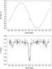 |
Fig. 2 The RV curve of the primary based on the mean RVs of the He ii lines (top) and the V light curve based on the ASAS3 data (bottom) compared with the final PHOEBE solution shown by solid lines. |
5. The KOREL disentangling
Since the 13 FEROS spectra are well distributed in the orbital phase, we decided to apply the disentangling technique; in the first step we used the programme KOREL (Hadrava 1995, 1997, 2004, 2005). We analysed the parts of the FEROS spectra covering the wavelength range from 4000 to 5100 Å. In particular, we formed three subsets in the neighbourhood of the Balmer lines Hδ, Hγ, and Hβ (4000 − 4175 Å, 4310 − 4400 Å, and 4800 − 4945 Å) and combined them into one KOREL input dataset. Similarly, we formed two subsets containing the neighbourhood of the He ii λ4541 and λ4686 lines (4495 − 4565 Å and 4670 − 4747 Å) and also combined them into another KOREL input dataset.
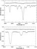 |
Fig. 3 Upper panel: the disentangled spectra of HD 165246 around Hδ. The secondary spectrum is shifted by +0.05. Note the presence of He i line λ4026 and Hδ in the secondary spectrum. Lower panel: the disentangled spectra around the He ii line λ4686. The secondary spectrum is shifted by +0.025. The He ii line is absent in the secondary spectrum. |
To see whether KOREL is able to detect weak lines of the secondary with some confidence, we first used the combined dataset containing all five subsets. Keeping the semiamplitude of the primary (which is well constrained by the direct RV measurements), eccentricity, and ω fixed at values from the PHOEBE solution, we investigated the run of the sum of squares of residuals as a function of the semiamplitude of the secondary K2. Regrettably, we could not find a trustworthy solution this way. This is not so surprising if one realizes that according to the PHOEBE solution, the secondary is for full 4m.6 fainter than the primary.
We therefore fixed all elements including the mass ratio of 0.173 from the PHOEBE solution and used KOREL only to disentangle the individual spectra. The programme KOREL returned very weak lines of the secondary for H i and He i lines and flat continua for the He ii lines. To the best of our knowledge, this goes beyond the current “record” by Holmgren et al. (1999), who detected a secondary for 4m.0 fainter than the primary in AR Cas. Two spectral segments of the disentangled spectra are shown in Fig. 3.
6. Spectroscopic analysis
6.1. Effective temperatures
The condition that the sum of the light factors, a relative contribution of the components to the total light of the system, is equal to unity constrains the search for the optimal parameters (Tamajo et al. 2011). In a new release of the computer programme for the constrained optimal fitting of disentangled component spectra, the following parameters could be adjusted for both components: the effective temperature, the surface gravity, the light dilution factor, Doppler shift, the projected rotational velocity, and the vertical shift to adjust for the continuum (in spectral disentangling, the disentangled component spectra are shifted and an additive factor should be applied to return them to the continuum level, cf. Pavlovski & Hensberge 2005). The comprehensive grids OSTAR and BSTAR of theoretical spectra calculated by Lanz & Hubeny (2003, 2007), were implemented for the optimal fitting. For the optimisation, a genetic algorithm is used (Charbonneau 1995). Further description of the code is given in Pavlovski et al. (2012, in prep.).
Only the hydrogen Balmer lines, Hδ, Hγ, and Hβ are selected for the optimal fitting. Due to the diffuse interstellar band centred on λ4882 (Herbig 1995) and affecting almost the whole red wing of Hβ, this line is only partially used. In fitting the line profiles of Hδ and Hγ, the blends due to various metal lines are also excluded. The surface gravities and light factors of both components were fixed at the values of the solution of Table 3.
Since the Balmer lines are almost insensitive to the rotational broadening with the exception of the very core of the lines, the projected rotational velocity was also fixed in these calculations. The projected rotational velocity was derived from the isolated helium lines in an iterative cycle by determining the effective temperatures from the Balmer lines. We arrived at v sini = 242.6 ± 2.7 km s-1. A strong correlation of Teff and log g occurs when fitting the Balmer line profiles. It is the major limitation in choosing the optimal model atmosphere and for subsequent abundance analysis. Fortunately, it is possible to derive accurate values of log g for both binary components from the combined light and velocity curve analysis for the eclipsing and double-lined spectroscopic binaries. Thanks to this, the degeneracy in Teff and log g can be lifted. In the present analysis, we therefore also fixed log g for both components at the values of Table 3.
Hence, the only free parameters that were optimized were the effective temperatures, Doppler shifts, and the vertical shifts. The mean values of the effective temperatures derived in these calculations individually for the three Balmer lines studied are Teff = 33 300 ± 400 K and Teff = 15 800 ± 700 K for the primary and secondary, respectively. The quality of the fits for the Hδ and Hγ lines can be judged from Fig. 4.
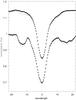 |
Fig. 4 A comparison of the disentangled and fitted line profiles of the Hγ (top) and Hδ (bottom) Balmer lines of the primary. Renormalised disentangled spectra are shown by black dots, while the best-fitting synthetic line profiles derived via optimisation in the OSTAR grid of non-LTE spectra calculated by Lanz & Hubeny (2003) are shown as solid lines. Blends conspicuous on hydrogen line profiles due to the various metals are not fitted. Theoretical spectra calculated for the solar abundance were used. |
6.2. Abundances
Theoretical spectra of the components were calculated in a “hybrid” approach with local thermodynamic equilibrium (LTE) atmospheres and non-LTE line formation (Nieva & Przybilla 2007). Model atmospheres were calculated with the atlas9 code. Non-LTE level populations and model spectra were obtained with detail and surface (Giddings 1981; Butler & Giddings 1985). Non-LTE-level populations and the synthetic spectra of H, He, C, N, O, Mg, and Si elements were computed using the most recent model atoms (cf. Table 3 in Nieva & Przybilla 2012).
The projected rotational velocity of the primary is rather high and the lines of metals are broad and shallow. The typical S/N of the input spectra is ~250, but the disentangling process enhances the S/N of disentangled individual spectra of the components because it works as a co-addition. Since the primary contributes more than 98% of the total light of the system, its disentangled spectrum gains about 3.5 times in the S/N, which means its disentangled spectrum has an S/N ~ 500. Therefore, in spite of broad and shallow metal lines that overlap and produce complex blends and spectral features, fine details can still be studied. We were able to trace spectral features down to 0.3% of the continuum level with confidence.
First, we estimated the microturbulent velocity. For hot, massive stars, oxygen and/or silicon lines serve this purpose since they are well populated in their spectra. In the present work, we have only used the silicon lines, neglecting the oxygen lines that occur only in complex blends.
Silicon is present in two ionisation stages, with the Si iv lines being much stronger than those of Si iii. Some of them are blended like Si iv λ4088.9 with oxygen lines and Si iv λ4631.2 with the carbon and oxygen lines. Yet, they are still strong enough to permit the abundance estimates. Minimizing the scatter in the abundances from different silicon lines, we obtained the microturbulent velocity ξt = 5 ± 1 km s-1. It eventually resulted in the abundance of silicon log ϵSi = 7.48 ± 0.08, in excellent agreement with recent comprehensive abundance studies of sharp-lined early B-type stars, log ϵSi = 7.51 ± 0.03 by Simón-Diaz (2010), log ϵSi = 7.50 ± 0.05 by Nieva & Przybilla (2012), and the Sun log ϵSi = 7.51 ± 0.03 (Asplund et al. 2009).
In accordance with the effective temperature of the primary, the helium lines are prominent in the optical spectrum and appear in two ionisation stages, He i and He ii. The strengths of He i lines correspond to the Teff of the primary, while the strengths of the synthetic He ii lines are too small in comparison to the disentangled line profiles. To obtain a satisfactory match, we would need to increase the model Teff by about 1500 K. We have no clear explanation for this discrepancy, which is also found for the spectra from the Lanz & Hubeny (2003) grid.
Table 4 contains the result of the helium abundance determination for the primary component from the most reliable He i lines. From the calculation point of view, the most trustworthy are the lines He i λ4471 and λ4920. The mean helium abundance for the primary component from the measured helium lines (Table 5) is ϵHe = 0.090 ± 0.010 or ϵHe = 0.089 ± 0.006 if only the two most reliable lines (He i λ4471 and λ4922) are considered. The quality of the fit for the studied He i lines can be judged from Fig. 5.
Abundance of helium derived from several He i lines.
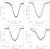 |
Fig. 5 Theoretical spectra of He i lines calculated for the atmospheric parameters of the primary component (Teff = 33 300 K, log g = 3.97, ξ = 5 km s-1) and three different abundances of helium (ϵ(He) = 0.08, 0.09 and 0.10) (solid lines) compared to the renormalised disentangled profiles of the helium lines of the primary component (black dots). |
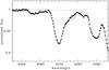 |
Fig. 6 Complex blends in the blue wing of Hδ line including lines of O ii (dotted), C iii (dashed), and Si iv (light grey solid). The composite spectrum for the abundances given in Table 4 represents the solid dark grey line. The renormalised, disentangled primary’s spectrum is shown by black dots. |
Abundances for the primary component of HD 165246.
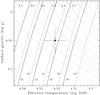 |
Fig. 7 Location of the primary component of HD 165246 in Teff vs. log g plane. Evolutionary tracks for models are labelled by their mass in the solar units. Evolutionary models by Brott et al. (2011) for the initial rotational velocities of v = 0 and 270 km s-1 are plotted as solid and dotted lines, respectively. Isochrones are plotted as solid and dotted thin lines. |
Abundances of other elements are estimated from the fitting of complex profiles. In Fig. 6, such a complex blend of O ii, C iii, and Si iv in the blue wing of Hδ line is shown. The final results are summarized in Table 5 and discussed in the following section.
7. Discussion
In Sect. 4, we found the fundamental quantities of the components of the binary system HD 165246. The more luminous component turned to be a high-mass star with M ~ 22 M⊙, R = 7.4 ± 0.2 R⊙, and a high rotational velocity v = 244 ± 3 km s-1. Therefore, this star is suitable for probing the predictive power of a new generation of stellar evolutionary models, with the rotation effects included in the calculations. Unfortunately, our analysis is hampered by the barely visible secondary’s spectrum and the rather limited number of available spectra. In conjunction with all-sky photometry, these were a limiting factor in matching the observations to the theoretical predictions.
In Fig. 7, the location of the primary component of HD 165246 in the log g–Teff plane is compared to the evolutionary calculations of the Utrecht group (Brott et al. 2011). The location of the primary corresponds to a mass about 1 M⊙ smaller than we assumed; nevertheless, it is an acceptable result. This is encouraging, but it still does not permit discrimination between the rotating and non-rotating evolutionary models, mainly because of the strong degeneracy of the models with respect to the initial rotational velocity. Another observational constraint is needed to distinguish between them. Since model calculations predict the most pronounced changes in nitrogen abundance, it is hoped that nitrogen can serve as another observable and eventually break down the degeneracy in the evolutionary tracks with respect to the initial rotational velocities.
From isochrones we estimated the age of the primary component τ ~ 3.3 ± 0.2 Myr with almost no difference between non-rotating and rotating evolutionary models, with the initial rotational velocities vsini = 0 and 270 km s-1.
Using the formulae by Zahn (1975, 1977) for the synchronization and circularization times, one gets 39 and 330 My, respectively. The reason why these times are so long is the small mass ratio. Therefore, the fast rotation is not surprising.
Rotating evolutionary models predict changes in the surface abundance pattern. Inspection of the Utrecht models for the mass of 20 M⊙ reveals that for the estimated age of the binary, τ ~ 3 Myr, the rotational velocity has not yet changed from its initial rotational velocity. Therefore, we consider the model with initial rotational velocity 271 km s-1 as closest to the measured primary’s rotational velocity, v ~ 244 km s-1. When compared with the initial chemical composition, we found that the model predicts the helium and nitrogen enrichment by 0.005 and 0.282 dex, respectively, and a depletion of carbon and oxygen by 0.089 and 0.017 dex, respectively. It is obvious that the change in the nitrogen abundance due to the rotational mixing should be detectable within the accuracy of the present abundance determination. The most robust indicator of the abundance change is the ratio of the nitrogen to carbon abundances, [N/C]. The model calculations predict changes from the initial [N/C] = − 0.49 to [N/C] = − 0.12 for the age of 4 Myr. Our abundance estimates for the primary give [N/C] = − 0.52 ± 0.08; hence, no changes in the abundances are detected. This result supports the previous findings for the high-mass stars in close binaries (Pavlovski & Southworth 2009; Pavlovski et al. 2009).
Abundances we derived in the present work for the primary component of HD 165246 (the second column in Table 5) are compatible with the cosmic abundance pattern of Nieva & Przybilla (2012) within their errors, except for the oxygen abundance. Further work on the larger sample of the stars in close binaries is needed to clarify this discrepancy.
We have found that the binary system HD 165246 contains a rapidly rotating high-mass star at an early stage of evolution. This star is an ideal object for probing the predictions of rotating evolutionary models. It is also an important object for the theory of binary-star origin since it is believed that the majority of the O-star binaries occurs in pairs with a mass ratio close to one (see, e.g., Chini et al. 2012, for details).
We therefore encourage both the more numerous high S/N and high-spectral-resolution spectroscopic observations and accurate multicolour photometry. Since HD 165246 is a relatively bright target, such observations could be obtained even with moderate-size telescopes.
The programme SPEL was written by the late Dr. J. Horn and never published. It was used in a number of publications, however, cf. Nemravová et al. (2012) and references therein.
Acknowledgments
We thank an anonymous referee, whose comments were very helpful. We profited from the use of the computerized bibliography maintained in the NASA/ADS system and the CDS in Strasbourg. The Czech authors were supported by the grant P209/10/0715 of the Czech Science Foundation and also by the research programme MSM0021620860. K.P. acknowledges support from the Croatian MZOS under research grant 119-0000000-3135.
References
- Arias, J. I., Barbá, R. H., Gamen, R. C., et al. 2010, ApJ, 710, L30 [NASA ADS] [CrossRef] [Google Scholar]
- Asplund, M., Grevesse, N., Sauval, J., & Scott, P. 2009, ARA&A, 47, 481 [NASA ADS] [CrossRef] [Google Scholar]
- Brott, I., de Mink, S. E., Cantiello, M., et al. 2011, A&A, 530, A115 [NASA ADS] [CrossRef] [EDP Sciences] [Google Scholar]
- Butler, K., & Giddings, J. 1985, Newsletter of Analysis of Astron. Spec., 9 (Univ. London) [Google Scholar]
- Charbonneau, P. 1995, ApJS, 101, 309 [NASA ADS] [CrossRef] [Google Scholar]
- Chini, R., Hoffmeister, V. H., Nasseri, A., Stahl, O., & Zinnecker, H. 2012, MNRAS, 424, 1925 [NASA ADS] [CrossRef] [Google Scholar]
- Garmany, C. D., Conti, P. S., & Massey, P. 1980, ApJ, 242, 1063 [NASA ADS] [CrossRef] [Google Scholar]
- Giddings, J. 1981, Ph.D. Thesis, Univ. London [Google Scholar]
- Gies, D. R., Fullerton, A. W., Bolton, C. T., et al. 1994, ApJ, 422, 823 [NASA ADS] [CrossRef] [Google Scholar]
- Hadrava, P. 1995, A&AS, 114, 393 [NASA ADS] [Google Scholar]
- Hadrava, P. 1997, A&AS, 122, 581 [NASA ADS] [CrossRef] [EDP Sciences] [Google Scholar]
- Hadrava, P. 2004, Publ. Astron. Inst. Acad. Sci. Czech Rep., 92, 15 [Google Scholar]
- Hadrava, P. 2005, Ap&SS, 296, 239 [NASA ADS] [CrossRef] [Google Scholar]
- Harmanec, P. 1988, BAC, 39, 329 [Google Scholar]
- Harmanec, P. 2003, in New Directions for Close Binary Studies: The Royal Road to the Stars, Publ. Canakkale Onsekiz Mart Univ., 3, 221 [Google Scholar]
- Herbig, G. H. 1995, ARA&A, 33, 19 [NASA ADS] [CrossRef] [Google Scholar]
- Holmgren, D. E., Hadrava, P., Harmanec, P., et al. 1999, A&A, 345, 855 [NASA ADS] [Google Scholar]
- Horn, J., Kubát, J., Harmanec, P., et al. 1996, A&A, 309, 521 [NASA ADS] [Google Scholar]
- Kraus, S., Weigelt, G., Balega, Y. Y., et al. 2009, A&A, 497, 195 [NASA ADS] [CrossRef] [EDP Sciences] [Google Scholar]
- Lanz, T., & Hubeny, I. 2003, ApJS, 146, 417 [NASA ADS] [CrossRef] [Google Scholar]
- Lanz, T., & Hubeny, I. 2007, ApJS, 169, 83 [CrossRef] [Google Scholar]
- Linder, N., Rauw, G., Sana, H., De Becker, M., & Gosset, E. 2007, A&A, 474, 193 [NASA ADS] [CrossRef] [EDP Sciences] [Google Scholar]
- Lucy, L. B., & Sweeney, M. A. 1971, AJ, 76, 544 [NASA ADS] [CrossRef] [Google Scholar]
- Martins, F., Schaerer, D., & Hillier, D. J. 2005, A&A, 436, 1049 [NASA ADS] [CrossRef] [EDP Sciences] [Google Scholar]
- Nemravová, J., Harmanec, P., Koubský, P., et al. 2012, A&A, 537, A59 [NASA ADS] [CrossRef] [EDP Sciences] [Google Scholar]
- Nieva, M. F., & Przybilla, N. 2007, A&A, 467, 295 [NASA ADS] [CrossRef] [EDP Sciences] [Google Scholar]
- Nieva, M. F., & Przybilla, N. 2012, A&A, 539, A143 [NASA ADS] [CrossRef] [EDP Sciences] [Google Scholar]
- Otero, S. A. 2007, OEJV, 72, 1 [Google Scholar]
- Pavlovski, K., & Hensberge, H. 2005, A&A, 439, 309 [NASA ADS] [CrossRef] [EDP Sciences] [Google Scholar]
- Pavlovski, K., & Southworth, J. 2009, MNRAS, 394, 1519 [NASA ADS] [CrossRef] [Google Scholar]
- Pavlovski, K., Tamajo, E., Koubský, P., et al. 2009, MNRAS, 400, 791 [NASA ADS] [CrossRef] [Google Scholar]
- Pojmanski, G. 2002, Acta Astron., 52, 397 [NASA ADS] [Google Scholar]
- Polidan, R. S., & Plavec, M. J. 1984, AJ, 89, 1721 [NASA ADS] [CrossRef] [Google Scholar]
- Prša, A., & Zwitter, T. 2005, ApJ, 628, 426 [NASA ADS] [CrossRef] [Google Scholar]
- Prša, A., & Zwitter, T. 2006, Ap&SS, 304, 347 [NASA ADS] [CrossRef] [Google Scholar]
- Simón-Diaz, S. 2010, A&A, 510, A22 [NASA ADS] [CrossRef] [EDP Sciences] [Google Scholar]
- Škoda, P. 1996, in Astronomical Data Analysis Software and Systems V, ASP Conf. Ser., 101, 187 [NASA ADS] [Google Scholar]
- Stickland, D. J., & Lloyd, C. 1999, The Observatory, 119, 16 [NASA ADS] [Google Scholar]
- Tamajo, E., Pavlovski, K., & Southworth, J. 2011, A&A, 526, A76 [NASA ADS] [CrossRef] [EDP Sciences] [Google Scholar]
- Trepl, L., Hambaryan, V. V., Pribulla, T., et al. 2012, MNRAS, 427, 1014 [NASA ADS] [CrossRef] [Google Scholar]
- Vaz, L. P. R., Cunha, N. C. S., Vieira, E. F., & Myrrha, M. L. M. 1997, A&A, 327, 1094 [NASA ADS] [Google Scholar]
- Walborn, N. R. 1972, AJ, 77, 312 [NASA ADS] [CrossRef] [Google Scholar]
- Williams, A. M., Gies, D. R., Bagnuolo, Jr., W. G., et al. 2001, ApJ, 548, 425 [NASA ADS] [CrossRef] [Google Scholar]
- Zahn, J.-P. 1975, A&A, 41, 329 [NASA ADS] [Google Scholar]
- Zahn, J.-P. 1977, A&A, 57, 383 [NASA ADS] [Google Scholar]
All Tables
RVs of six strong spectral lines of the primary of HD 165246 measured on the FEROS spectra in SPEFO.
Preliminary orbital solutions on RVs of several spectral lines measured directly in SPEFO.
All Figures
|
Fig. 1 Line profiles of the He i λ4471 line at phases close to quadratures. |
| In the text | |
|
Fig. 2 The RV curve of the primary based on the mean RVs of the He ii lines (top) and the V light curve based on the ASAS3 data (bottom) compared with the final PHOEBE solution shown by solid lines. |
| In the text | |
|
Fig. 3 Upper panel: the disentangled spectra of HD 165246 around Hδ. The secondary spectrum is shifted by +0.05. Note the presence of He i line λ4026 and Hδ in the secondary spectrum. Lower panel: the disentangled spectra around the He ii line λ4686. The secondary spectrum is shifted by +0.025. The He ii line is absent in the secondary spectrum. |
| In the text | |
|
Fig. 4 A comparison of the disentangled and fitted line profiles of the Hγ (top) and Hδ (bottom) Balmer lines of the primary. Renormalised disentangled spectra are shown by black dots, while the best-fitting synthetic line profiles derived via optimisation in the OSTAR grid of non-LTE spectra calculated by Lanz & Hubeny (2003) are shown as solid lines. Blends conspicuous on hydrogen line profiles due to the various metals are not fitted. Theoretical spectra calculated for the solar abundance were used. |
| In the text | |
|
Fig. 5 Theoretical spectra of He i lines calculated for the atmospheric parameters of the primary component (Teff = 33 300 K, log g = 3.97, ξ = 5 km s-1) and three different abundances of helium (ϵ(He) = 0.08, 0.09 and 0.10) (solid lines) compared to the renormalised disentangled profiles of the helium lines of the primary component (black dots). |
| In the text | |
|
Fig. 6 Complex blends in the blue wing of Hδ line including lines of O ii (dotted), C iii (dashed), and Si iv (light grey solid). The composite spectrum for the abundances given in Table 4 represents the solid dark grey line. The renormalised, disentangled primary’s spectrum is shown by black dots. |
| In the text | |
|
Fig. 7 Location of the primary component of HD 165246 in Teff vs. log g plane. Evolutionary tracks for models are labelled by their mass in the solar units. Evolutionary models by Brott et al. (2011) for the initial rotational velocities of v = 0 and 270 km s-1 are plotted as solid and dotted lines, respectively. Isochrones are plotted as solid and dotted thin lines. |
| In the text | |
Current usage metrics show cumulative count of Article Views (full-text article views including HTML views, PDF and ePub downloads, according to the available data) and Abstracts Views on Vision4Press platform.
Data correspond to usage on the plateform after 2015. The current usage metrics is available 48-96 hours after online publication and is updated daily on week days.
Initial download of the metrics may take a while.