© ESO, 2013

1. Introduction

Understanding the excitation mechanisms and drivers in nearby starburst galaxies is critical to understanding their role in galaxy evolution. One of the best laboratories to study this is NGC 253. This galaxy is a nearby (3.5 Mpc Rekola et al. 2005), edge-on infrared bright galaxy that is part of the Sculptor group. It is classified as a late-type barred spiral galaxy (SAB(s)c) with star formation confined to the inner 0.5 kpc. The star formation rate of the starburst is 1.4−9.5 M_⊙ yr^-1 (Grimm et al. 2003). This intense episode of star formation is driven by a 7 kpc bar, which funnels gas into the nucleus (Engelbracht et al. 1998). There is a starburst driven superwind extending perpendicular to the disk (Demoulin & Burbidge 1970; Ulrich 1978; Fabbiano & Trinchieri 1984; McCarthy et al. 1987; Westmoquette et al. 2011).

The inner region of star formation is highly obscured with an A_V of  ~5−18 mag (Kornei & McCrady 2009; Fernández-Ontiveros et al. 2009). Many dense, luminous, dust enshrouded young stellar clusters have been found in the nucleus (Forbes et al. 1993, 2000). In addition to the stellar clusters, Alonso-Herrero et al. (2003) and Ulvestad & Antonucci (1997) have observed many compact radio sources in [FeII] and radio respectively, representing young supernova remnants. Turner & Ho (1985) observed over 60 compact radio sources, the brightest of which is named TH2. A high resolution (1′′ − 2′′) study of the molecular gas in NGC 253 was performed by Sakamoto et al. (2011). They found 5 warm, dense clumps of molecular gas, which are all coincident with radio sources. They suggest that these clumps are natal molecular cloud complexes harboring massive star formation. The K band continuum peak, which was originally defined as the nucleus by Forbes et al. (1991), is the location of a super star cluster. This super star cluster was observed with Hubble Space Telescope by Watson et al. (1996) and is consistent with a single stellar population. In the mid infrared, two bright peaks have been observed in the central regions. The brightest of the two is coincident with the K band continuum peak and super star cluster and has no radio counterpart (Ulvestad & Antonucci 1997). The second, 3.0′′ to the northeast is coincident to the radio peak TH2. A more recent study by Ulvestad & Antonucci (1997) suggests that TH2 is the true nucleus of NGC 253 and represents either a low-luminosity active galactic nucleus (AGN) or a compact supernova remnant.

Although TH2 is generally considered to be the nucleus, a recent study by Müller-Sánchez et al. (2010) provides new estimates for the kinematic center based on the kinematics of the stellar component. Using SINFONI on the VLT, they were able to achieve very high angular resolution and derive the stellar velocity field. They found the kinematic center to be offset from TH2 only by $\mathrm{\Delta }\mathit{x}\mathrm{=}\mathrm{0}\stackrel{\mathrm{″}}{.}\mathrm{6}$ and $\mathrm{\Delta }\mathit{y}\mathrm{=}\mathrm{0}\stackrel{\mathrm{″}}{.}\mathrm{4}$ (i.e. by 12 pc) in the southwest direction. They propose an alternative position for the kinematic center as the X-ray source X-1 (Weaver et al. 2002). Although NGC 253 has been the target for many detailed kinematic studies, there is still much uncertainty about the precise location of the true kinematic center.

The subject of excitation mechanisms has been extensively studied in NGC 253. Martín et al. (2006) finds that the chemistry and heating of NGC 253 is dominated by large scale, low velocity shocks. Presence of shocked molecular material is indeed evident through the presence of widespread SiO emission throughout the nuclear regions (García-Burillo et al. 2000). Martín et al. (2009b) suggest that, although NGC 253 is dominated by shock chemistry, photon-dominated regions (PDRs) play a crucial role in the chemistry, since there are very high abundances of PDR tracing molecules, namely HCO⁺, CO⁺. In addition, they find that although NGC 253 was thought to be at an earlier stage of evolution than M 82, a prototypical starburst with strong PDR characteristics, the molecular clouds are larger and have a higher column density, pointing to a later stage of evolution, such as seen in M 82. Martín et al. (2009a) also find that the ultraviolet (UV) heating in NGC 253 is more similar to M 82 than other starbursts, yet still not the dominant excitation mechanism. Harrison et al. (1998) used the ortho- to para- ratio of H₂, to argue that most of the H₂ is excited by PDRs instead of shocks. In addition, Israel et al. (1989); Luhman et al. (1994) show in NGC 604 and Orion A respectively that although in small-beam apertures it may seem as if high surface brightness H₂ emission from shocks is dominant, when the beam size increases, it is clear that fluorescent excitation dominates on large scales.

In this paper, we investigate the excitation mechanisms for the molecular gas in the nuclear region of NGC 253. We use the following methods to differentiate between shock dominated and PDR dominated excitation on a 2 pc scale:

• Calculate the 2-1 S(1)/1-0 (S1) line ratio at each pixel position

• Compare morphology of Brγ, [FeII], and polycyclic aromatic hydrocarbons (PAHs) to that of the H₂

• Relate observed H₂ excitation diagrams to those generated by shock and PDR models.

In Sect. 2, we will discuss the observations, while in Sect. 3 we present the derived spectra and linemaps. In Sect. 4 we will investigate and define the kinematic center. Then, in Sect. 5, we investigate the nature of the dominant excitation mechanisms throughout the galaxy, focusing on the dense clumps. In Sect. 6, we compare our excitation diagrams to shock and PDR models spanning the parameter space. We summarize our conclusions and their implications in Sect. 7.

2. Observations

2.1. SINFONI observations

All observations were made with the Spectrograph for INtegral Field Observations in the Near-Infrared (SINFONI) at the ESO VLT. SINFONI provides spatial and spectral data in the form of data cubes in J, H, and K bands. The SINFONI instrument is mounted at the Cassegrain focus of the Unit Telescope 4 at the Very Large Telescope (VLT).

We observed in the H, and K bands using a spatial pixel scale of 0.25′′ corresponding to a field of view of 8′′  × 8′′ per frame and a spectral resolution of 2000, 3000 and 4000 respectively, which corresponds to a velocity resolution of 149.8, 99.9 and 74.9 km s^-1. All science observations were taken in the ABA’nodding mode (300 s of object, 300 s of sky, 300 s of object), where A′ is slightly offset from A. The object exposures are aligned and averaged during the reconstruction of the data cube.

The observations of NGC 253 were made in visitor mode on August 28th, 2005. In order to capture the full extent of the H₂ emission, consecutive frames were taken in the K band moving further away from the center, along the disk until H₂ was no longer detected. This resulted in 6 separate pointings. Since there are also H₂ transitions in the H band, a similar strategy was used, resulting in 4 separate pointings.

We used the standard reduction techniques of the SINFONI pipeline on all observations. including corrections for flat field, dark current, nonlinearity of pixels, distortion, and wavelength calibration. We obtained the flux calibration and atmospheric corrections from observations of a standard star, namely HR 2058 in the H band and HD 20001 in the K band. This is the same dataset Müller-Sánchez et al. (2010) used to determine the kinematic center.

2.2. ISAAC observations

We use the ISAAC observations of NGC 253 in the 3.21 and 3.28 μm filters described by Tacconi-Garman et al. (2005). These observations were uncalibrated. We established a flux calibration for these two images using the ISO-SWS spectra by Sturm et al. (2000), taking into account the filter profiles of the two ISAAC filters and the precise location and orientations of the ISO-SWS aperture. Inspection of the spectrum by Sturm et al. (2000) shows that the 3.21 μm filter contains only continuum emission, while the 3.28 μm filter contains continuum+PAH emission. The peak of the PAH emission is at 3.3 μm, which is fully included in the 3.28 μm filter. The spectral slope is small enough that there is negligible change in continuum level between 3.21 and 3.28 μm and therefore a PAH emission image was created by subtracting the calibrated 3.21 μm image from the calibrated 3.28 μm image.

3. Results

The SINFONI datacubes allow us to construct continuum maps, line maps and velocity maps of emission lines detected in these bands. The K band continuum map and H₂ 1-0 S(1) emission line map are shown in Fig. 1 and the Brγ and [FeII]_1.64 emission line maps are shown in Fig. 2. All line maps are centered on the kinematic center proposed by Müller-Sánchez et al. (2010). We have chosen 8 regions defined by the most dominant H₂ peaks and these regions are overplotted by white rectangles in each map. There is an additional region centered on the kinematic center. All regions are 12 × 12 pixels or 1.5 × 1.5 arcsec. These regions were selected based on H₂ flux. There is a relatively bright H₂ emission clump to the north west of Region 1, which was not selected for analysis since it shows similar emission features to Region 1.

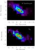Fig. 1 K band continuum map and H2 1-0 S(1) line map of NGC 253. The offset from the kinematic center at position $\mathrm{(}\mathit{\alpha ,\delta }{\mathrm{)}}_{\mathrm{2000}}\mathrm{=}\mathrm{(}{\mathrm{00}}^{\mathrm{h}}{\mathrm{47}}^{\mathrm{m}}\mathrm{33}\stackrel{\mathrm{s}}{.}\mathrm{14}\mathit{,}\mathrm{-}{\mathrm{25}}^{\mathrm{◦}}{\mathrm{17}}^{\mathrm{\prime }}\mathrm{17}\stackrel{\mathrm{″}}{.}\mathrm{52}\mathrm{)}$ is given on each axis. The contours represent 13 equally spaced levels with a maximum flux of 1.3 × 10-11 erg s-1 cm-2  μm-1 arcsec-2 and 5.4 × 10-15 erg s-1 cm-2 arcsec-2, for the K band continuum and H2 respectively. The white rectangular regions are H2 flux peaks, with the exception of Region 3, which is centered on the kinematic center. The blue “+” represents the kinematic center, the blue triangle represents X-1 and the blue diamond represents TH2.

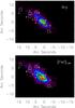Fig. 2 Brγ and [FeII]1.64 emission line map of NGC 253. The offset from the kinematic center at position $\mathrm{(}\mathit{\alpha ,\delta }{\mathrm{)}}_{\mathrm{2000}}\mathrm{=}\mathrm{(}{\mathrm{00}}^{\mathrm{h}}{\mathrm{47}}^{\mathrm{m}}\mathrm{33}\stackrel{\mathrm{s}}{.}\mathrm{14}\mathit{,}\mathrm{-}{\mathrm{25}}^{\mathrm{◦}}{\mathrm{17}}^{\mathrm{\prime }}\mathrm{17}\stackrel{\mathrm{″}}{.}\mathrm{52}\mathrm{)}$ is given on each axis. The contours represent 13 equally spaced levels with a maximum flux of 4.5 × 10-14 and 2.8 × 10-14 erg s-1 cm-2 arcsec-2 for Brγ and [FeII] respectively. The white rectangular regions are areas of concentrated H2 flux, with the exception of Region 3, which is centered on the kinematic center.

The K band continuum map reveals the inclined disk of the galaxy, tracing the older stellar population. The disk appears irregular with clear clumps of high luminosity. The kinematic center (Region 3) shows a very high level of continuum emission. In addition, superimposed on the bright continuum emission around the kinematic center, there is a bright flux peak at the location of the super star cluster (Region 2) studied by Watson et al. (1996).

On the other hand, the H₂ 1-0 S(1) map shows a completely different morphology. The H₂ extends along the entire disk with its brightest clump located several arcseconds east of the kinematic center (Region 3). However, the H₂ is even more inhomogeneous than the K band continuum. There are clear H₂ bright clumps ranging out into the furthest regions. The white rectangles highlight the brightest emission clumps. There is also significant H₂ emission originating from the super star cluster (Region 2), but not from the center.

Similarly, comparison of the H₂ and the Brγ map reveals little correlation. The Brγ flux peak is coincident with the super star cluster, but shows no clear flux increase near Region 4, where H₂ is brightest, nor at the center. The Brγ is also generally less extended than the H₂, with most of the emission in the southwestern portion of the galaxy, centered on the super star cluster.

The [FeII]_1.64 map also reveals emission peaking near, but not coincident with, Region 4. In the northeastern regions, the [FeII] emission is also quite clumpy, with some of the clumps coinciding with the H₂, such as Regions 5, 7 and 8. Comparing the [FeII] to the Brγ emission, we see in both cases, as well as in the K continuum, an elongated arm-like feature coming from the center, curving out towards the northeast corner along the disk, bordering on the northern edge of Region 5. However the [FeII] feature is spatially offset towards the south with respect to the Brγ feature, as noted originally by Forbes et al. (1993). The H₂ and continuum emission in this region traces neither Brγ or [FeII].

Figure 3 displays the rest-frame K band spectra, integrated over the regions shown on the H₂ map (Fig. 1). The main emission lines are highlighted. Specifically, we see many H₂ transitions as well as Brγ and HeI. The highest energy H₂ transition detected is the 3-2 S(3) transition. This is located at 2.2008 μm and only marginally visible in Region 8 of Fig. 3, although we have 2σ detections of it in Regions 1, 2, and 3. This is an important detection since this transition can only be excited by high energy photons, and therefore points towards fluorescent excitation. In Table 1 we present the integrated fluxes and fluxes in each region of all detected H₂ lines with error bars. These error bars were derived by calculating the flux for a range of different continuum baselines and finding the standard deviation of these values. We also attempted to extract H₂ line fluxes from transitions in the H band, yet the stellar absorption features overpowered the emission lines and we were unable to get reliable flux measurements.

Using the SINFONI data cubes, we can extract both a gas and stellar velocity map. Figure 4 displays the stellar velocity field with the H₂ molecular gas velocity field in contours. The stellar velocity field was calculated by fitting the three stellar CO photospheric absorption features. Fitting with a set of 6 template stars (K3V, M0III, M0V, M4V, M5III and M5II), we used the Cappellari & Emsellem (2004) Penalised Pixel Fitting (PPXF) package. All the template stars were observed with SINFONI on the same settings as the NGC 253 observations. In addition, the pixels were binned using a Voronoi tessellation (Cappellari & Copin 2003), with a signal-to-noise of 50 per bin. These binned spectra were then fit with the best combination of the 6 template stellar spectra varying velocity and dispersion. Then, the systemic velocity of the galaxy, 243 km s^-1, was subtracted from the velocity field.

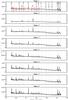Fig. 3 K band spectra of H2 bright clumps. The integrated K band spectra, in the rest frame, integrated over the regions shown in Fig. 1. Vertical dotted lines are used to show dominant emission lines. The strongest OH lines have been marked in the spectrum of Region 1 with the red dot-dash line. The 12CO absorption bands are also visible at 2.294, 2.323, and 2.353 μm respectively. Region 2 is the K Continuum peak and hot spot, Region 3 is the kinematic nucleus, and Region 4 is the H2 emission peak.

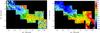Fig. 4 Stellar velocity field (left) with H2 1-0 S(1) velocity contours and H2 1-0 S(1) velocity map with contours (right). The contour levels are  − 75, − 50, − 30, − 10,0,10,30,50,75 km s-1. The color bar describes the H2 and stellar velocity in km s-1. On the right panel, the red circle represents the 3σ uncertainty for the center defined by Müller-Sánchez et al. (2010). The plus sign is the center of this circle, and the kinematic center. The diamond is TH2, the radio peak. The triangle is X-1, the X-ray peak. The square is the point of highest symmetry.

4. The kinematic center of NGC 253

The stellar velocity field and the H₂ velocity field show many general similarities, especially in the central region. Specifically, both the stellar and gas velocity fields show an “S”-shaped morphology in the velocity contours in the 0 km s^-1 range. This morphology is typical of galaxies with a bar potential, and supports the claim of a bar potential in NGC 253.

Since the H₂ velocity field is much cleaner than the stellar velocity field and they share a similar morphology, we will use the H₂ velocity to estimate the kinematic center of NGC 253. In order to estimate this position, we create a mirrored reflection around a set of central points that could be the center. By subtracting this mirrored map from the original map, we can find which pixel provides the most symmetric profile. Using this method, we can determine the center pixel, or the pixel with the most symmetry. To determine the absolute coordinates of this pixel, we employ the 2MASS K band image of NGC 253. We anchor the SINFONI observations to the 2MASS observations by finding the position of the K-band peak. We then use the offset of the kinematic center to the K band center to determine the absolute coordinates, $\mathrm{(}\mathit{\alpha ,\delta }{\mathrm{)}}_{\mathrm{2000}}\mathrm{=}\mathrm{(}{\mathrm{00}}^{\mathrm{h}}{\mathrm{47}}^{\mathrm{m}}\mathrm{33}\stackrel{\mathrm{s}}{.}\mathrm{084}$, $\mathrm{-}{\mathrm{25}}^{\mathrm{◦}}{\mathrm{17}}^{\mathrm{\prime }}\mathrm{18}\stackrel{\mathrm{″}}{.}\mathrm{42}$). Müller-Sánchez et al. (2010) find the kinematic center at $\mathrm{(}\mathit{\alpha ,\delta }{\mathrm{)}}_{\mathrm{2000}}\mathrm{=}\mathrm{(}{\mathrm{00}}^{\mathrm{h}}{\mathrm{47}}^{\mathrm{m}}\mathrm{33}\stackrel{\mathrm{s}}{.}\mathrm{14}\mathit{,}\mathrm{-}{\mathrm{25}}^{\mathrm{◦}}\mathrm{17}\prime \mathrm{17}\stackrel{\mathrm{″}}{.}\mathrm{52}\mathrm{)}$ with a mean 3σ error of r = 1.2″. Thus, our center is within this error and in good agreement with their result. The difference between the two results is due to the method. Muller-Sanchez used an inclined disk model to find their kinematic center, however the symmetry argument focuses on finding the point of highest symmetry. This method is compromised due to two symmetric circular regions in the velocity field, the top circle is located within the red error circle and the symmetric counterpart is just below it and appears green. Our method finds the center to be just between these two circles, at the radius of the Muller-Sanchez error radius, represented as a square. Due to this symmetric point, we consider the Muller-Sanchez center to be the true kinematic center, which is also clear from the inflection point of the bar profile “S” shape seen in the H2 velocity field. Since the H2 inflection point coincides perfectly with the Muller-Sanchez center, it proves that there is no true offest between the H2 and CO measured centers.We therefore independently confirm the kinematic center proposed by Müller-Sánchez et al. (2010). In Fig. 4, the H₂ 1-0 S(1) velocity map is presented with the Müller-Sánchez et al. (2010) 3σ center circled in red and their proposed kinematic center overlaid with a white plus sign. For completeness, the radio peak TH2 and the x-ray peak X-1 are both overplotted as a diamond and triangle respectively.

5. Gas excitation mechanisms in NGC 253

In general, the morphologies of the K band continuum, H₂, Brγ, and [FeII]_1.64 emission are dissimilar. None of the peaks are coincident with each other with the exception of the K band and Brγ peaks at the super star cluster. There are certain regions where the H₂ matches the Brγ, while some H₂ clumps match the [FeII]_1.64 emission. This suggests that the H₂, Brγ and [FeII] are being excited through different physical processes.

The Brγ peak, tracing massive, young star formation, is coincident with the K band continuum peak, at the location of the super star cluster. In general, the K band continuum traces the older medium and low mass populations of stars in contrast to the youngest, most massive stars powering the Brγ emission. There is extended emission in the northeastern direction of the Brγ peak, but no other strong emission regions.

[FeII] is another strong NIR diagnostic line, which traces shocks. In interstellar space, iron atoms are typically fully locked into dust grains. Shock fronts associated with supernova remnants (SNRs) may cause very efficient grain destruction through thermal sputtering (Jones et al. 1994). This releases the iron into the gas-phase where it is singly ionized by the interstellar radiation field (Mouri et al. 2000). In the extended post shock region, Fe⁺ is excited by electron collisions, rendering it a strong diagnostic shock tracer. The [FeII] peak is located slightly northeast of the H₂ peak (Region 4). It shows diffuse emission consistently along the disk, but does not show any peak at Region 2, the location of the super star cluster. From Rosenberg et al. (2012) we can calculate the supernova rate (SNrate) from the FeII luminosity. In Table 2 the calculated SNrates for each region and the whole galaxy is given. The small amount of [FeII] flux and correspondingly low supernova rate suggests that the super star cluster in Region 2 is a young cluster. Fernández-Ontiveros et al. (2009) suggests that Region 2 is a starburst of 6 Myr, which is also consistent with our age calculations. Our integrated supernova rate in the inner 300 pc of the galaxy, is 0.2 yr^-1, which is well matched to previous supernova rate measurement of 0.1 − 0.3 (Rieke et al. 1980, 1988; Ulvestad & Antonucci 1997).

Unlike Brγ and [FeII], the mechanism which excites the H₂ gas is not as clear. The NIR is rich with ro-vibrational H₂ lines, which can either be excited thermally, through shocks, or by fluorescence, through UV photons from O and B stars. In the case of shock excited H₂ emission, the gas is thermalized and the energy levels are populated in a “bottom-up” manner. The resulting gas temperature is around 1000 K and thus there is little H₂ emission from the v ≥ 3 states, which have temperatures above 15 000 K. However, in the case of excitation by UV photons, the H₂ molecule absorbs a highly energetic photon and is excited to an upper electronic energy level and then proceeds to cascade downwards. This is considered populating the energy levels from the “top-down”, which results in exciting higher H₂ energy levels. In this way, we can use the ratio of certain H₂ lines to discriminate which excitation mechanism is exciting the H₂ emission. However, the case of UV excitation is sometimes degenerate. In the case of high density, the molecules can collide frequently enough to become thermalized in the lower energy levels, which results in line ratios equivalent to the case of shock excitation. For the lines to be thermalized, the density in the region must be comparable to the critical density of the lines, 1.7 × 10⁵ cm^-2 for 1-0 S(1) and 1.2 × 10⁵ cm^-2 for 2-1 S(1) (Sternberg & Dalgarno 1989).

In order to determine which excitation mechanisms are dominating which regions, we can use the information from the Brγ and [FeII] tracers. Specifically, if the H₂ is undergoing excitation by UV photons in a dense environment, this region should also be bright in Brγ emission if the excitation is by O stars. Conversely, if the H₂ is being excited by shocks, then the [FeII] emission might also be bright in this region.

In Region 2, coincident with the Brγ peak, UV photon excitation is the dominant mechanism and the density of this region is accounting for the lower excitation levels being populated leading to the lower H₂ line ratio. In Region 6, there is little Brγ emission. However, the [FeII] emission shows a bright clump. Therefore, in this region the emission lines suggest that the H₂ is being excited by shocks. However, in the other regions, there is both diffuse [FeII] and diffuse Brγ. In this case, we cannot determine the dominant mechanism by only studying the Brγ and [FeII] emission. Since H₂ can also be excited by slow shocks, too slow to destroy dust grains, or by B stars, which are not energetic enough to excite Brγ, we must use other diagnostics to probe the excitation mechanisms.

One diagnostic is the 2-1 S(1) to 1-0 S(1) transitions at 2.2478 μm and 2.1218 μm respectively. This line ratio is commonly used because both lines are relatively bright and have similar wavelengths, so they can usually be taken in the same spectrum and suffer identical extinctions. Predictions for the ratio of these two lines due to excitations by shocks range from 0.1 to 0.2 (Shull & Hollenbach 1978), while for photo-excitation it is predicted to be 0.53 − 0.56 (Black & van Dishoeck 1987).

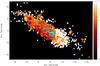Fig. 5 The ratio of 2-1 S(1)/1-0 S(1) H2 lines with the Brγ line map over plotted in contours. The white rectangles are the same regions as defined in Fig. 1. The color bar values represent the value of the ratio. The offset from the kinematic center at position $\mathrm{(}\mathit{\alpha ,\delta }{\mathrm{)}}_{\mathrm{2000}}\mathrm{=}\mathrm{(}{\mathrm{00}}^{\mathrm{h}}{\mathrm{47}}^{\mathrm{m}}\mathrm{33}\stackrel{\mathrm{s}}{.}\mathrm{14}\mathit{,}\mathrm{-}{\mathrm{25}}^{\mathrm{◦}}\mathrm{17}\prime \mathrm{17}\stackrel{\mathrm{″}}{.}\mathrm{52}\mathrm{)}$ is given on each axis. Ratio values where the line flux of either transition is below 10% of the maximum flux of that line are masked.

5.1. Shocks vs. fluorescence

In Fig. 5, we present a map of the 2-1 S(1)/1-0 S(1) ratio with the contours of the Brγ line map and the rectangular regions from Fig. 1 overlaid. The 2-1 S(1) line is significantly weaker than the 1-0 S(1) transition thus this image has less signal-to-noise. We have therefore applied a mask to the map, filtering out values lower than 10% of the maximum flux for both line transitions. The values of the 2-1 S(1)/1-0 S(1) ratio range continuously from 0 to 0.5, showing that we have both thermalized and fluorescently excited gas in the galaxy. Both the mean H₂ ratio for each region and the ratio of the integratred 2-1 S(1) and 1-0 S(1) line fluxes is listed in Table 3. The discrepency in these two values is due to the fact that in the left column, we find the mean value of the H₂ ratio at each pixel for each region, whereas in the right column we first integrate the flux in each region for the two lines, and then divide the fluxes. The latter method is more sensitive to high surface brightness quantities, and shocks excited material has higher surface brightness than that of fluorescent excitation (Shull & Hollenbach 1978). Therefore, the values in the right column are weighted towards shock excitation, and thus show lower ratios for each region. Averaging the ratio on a pixel-by-pixel basis, as done in the left column, does not present such a bias. In regions with very high ratios ( ≥ 0.3) we can confidently conclude that the molecular hydrogen is being excited by UV photons from O and B stars. Similarly, there are a few regions where the ratio is distinctly lower than the average value of  ~ 0.2. These regions are region 2, 6, and 7 from Fig. 5. It is interesting to note that these bright regions all correlate with an H₂ clump or luminosity peak. In these regions we cannot determine whether the low H₂ line ratio is indicating excitation by shocks, or a very dense clump being excited by UV photons. However, we can place an upper limit on the amount of shocked gas. Assuming that all gas with a 2-1 S(1)/1-0 S(1) ratio lower than 0.2 is shock excited, we see that 48% of the total 1-0 S(1) H₂ flux may be from “shocked” gas. However, this percentage is including all regions with a ratio lower than 0.2, including regions of high density where the gas is fluorescently excited but thermalized. We can at least partially separate this effect by filtering out the pixels with the highest Brγ flux ( ≥ 1 × 10^-16 erg s^-1 cm^-2), since these regions are dense regions of known fluorescent excitation. As seen in the Brγ contours in Fig. 5, this affects Regions 2, 3, and 4. Excluding these regions and any pixel with high Brγ flux, no more than 29% of all H₂ is shock excited, and the actual amount may be less.

5.2. Tracers of fluorescence

If strong shocks dominate the excitation of H₂ in NGC 253, we would expect to see a good correlation between H₂ and [FeII], which we do not. If fluorescence is the dominant mechanism, we would expect the Brγ morphology to share more similarities with that of the H₂. We also see no correlation between H₂ and Brγ emission. However, Brγ only traces the most massive and young stars, predominately the O stars. In order to excite Brγ, the star must emitting Lyman continuum photons (λ < 912   Å, 13.6 eV), yet H₂ can be excited by lower energy photons as well (λ < 1100   Å, 11.2 eV).

Similarly to H₂, polycyclic aromatic hydrocarbons (PAHs) have a lower excitation energy than HI (λ ~ 4200   Å for N_C > 50 where N_C > 50 is the number of carbon atoms; Bakes & Tielens 1994) and thus are excited not only by O stars but also by slightly less massive, B-type stars. Therefore, the PAH emission traces the more general fluorescently excited population, including excitation by both O and B stars. By comparing the morphology of the H₂ to that of PAH emission, we can determine if it is indeed the B stars that are predominately responsible for exciting the H₂ regions, and why neither the Brγ, [FeII] or K band continuum matches its morphology.

In Fig. 6, we present an ISAAC continuum subtracted PAH map at 3.21 μm. The left panel is overlaid with H₂ 1-0 S(1) contours, the middle panel is overlaid with Brγ contours, and the right panel is overlaid with [FeII]_1.64 contours. The two maps were centred with respect to one another by matching the K band continuum peak of the SINFONI maps to the 3.21 continuum peak of the ISAAC continuum maps.

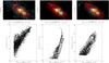Fig. 6 Top panels: PAH 3.28 μm continuum subtracted image from ISAAC. Left panel has H2 1-0 S(1) contours, middle panel has Brγ contours, right panel has [FeII]1.64 contours. The offset from the kinematic center at position $\mathrm{(}\mathit{\alpha ,\delta }{\mathrm{)}}_{\mathrm{2000}}\mathrm{=}\mathrm{(}{\mathrm{00}}^{\mathrm{h}}{\mathrm{47}}^{\mathrm{m}}\mathrm{33}\stackrel{\mathrm{s}}{.}\mathrm{14}\mathit{,}\mathrm{-}{\mathrm{25}}^{\mathrm{◦}}{\mathrm{17}}^{\mathrm{\prime }}\mathrm{17}\stackrel{\mathrm{″}}{.}\mathrm{52}\mathrm{)}$ is given on each axis. The kinematic center is from Müller-Sánchez et al. (2010). Bottom panels: pixel-pixel plots of PAH flux vs. H2 flux (left), Brγ flux (center), and [FeII] flux (right). The pixels of the ISAAC PAH observations were rebinned to match those of the SINFONI observations.

From these images, the morphology of the PAH emission matches the H₂ emission, better than both the Brγ and [FeII]. The Brγ peak is coincident with secondary PAH peak, meaning that in this region, there are many O stars producing photons E > 13.6   eV. However, there is little Brγ emission coincident with the primary PAH peak, showing that these regions are mainly excited by B stars. The [FeII] peak shows little similarity to the PAH emission. However, the H₂ peaks are coincident with both the primary and secondary PAH peaks and shares a generally similar morphology in the diffuse PAH emission. It is interesting to note that the elongated feature seen in the K Continuum, [FeII] and Brγ maps in Fig. 2, is also present in the PAH map, but not in the H₂. Since we still have a high amount of diffuse emission in this region, it is most likely that there is H₂ emission originating from this feature, but it is just relatively dimmer than the nearby H₂ peaks, which therefore overshadow it.

In order to test this correlation in a more quantitative sense, we can perform a pixel-pixel analysis of the correlation of our line maps to that of the PAH 3.21 μm emission. After re-binning the ISAAC PAH map to match the pixel size of SINFONI, we plot the flux of H₂, Brγ and [FeII] as compared to the PAH flux. Figure 6 depicts these correlation plots, which show how well H₂, Brγ and [FeII] correlate with the PAH flux. The Brγ vs. PAH plot shows an interesting morphology, in which the emission seems to be coming from two different areas. First, there is an approximately linear correlation for lower Brγ fluxes. This correlation is most likely due to the diffuse Brγ emission caused by the same photons exciting the PAHs. However, there is a second, non-linear, nearly vertical component of extremely high Brγ flux and medium strength PAH flux. These points correspond to the location of the super star cluster, which is only the secondary flux peak for PAH, but the dominating source of Brγ flux. The [FeII] also seems to correlate with PAH flux with a large, but constant spread, suggesting that these tracers originate in the same general region but without a direct physical correlation, emphasized by the displacement of the [FeII] peak and the PAH peak. The H₂ also shows a linear correlation with the PAH flux. However, this correlation has a very large spread at low fluxes and gets continually tighter as both H₂ and PAH fluxes increase. We can see this same trend in the morphologies as well. There is a strong correlation, both spatially and numerically for the peaks of the H₂ and PAH linemaps, however in the diffuse regions the correlation no longer holds.

The strong, linear correlation between H₂ and PAH morphology in the central region of NGC 253 gives added confidence that most of the central emission in NGC 253 (Regions 2, 3, and 4) is fluorescently excited. In addition, the correlation between the PAH morphology and H₂ morphology indicates that the H₂ in this area, is being excited by the same stars that are exciting the PAHs, mainly B-type stars.

6. PDR and shock models

Although the morphological correlation of H₂ to fluorescently excited PAHs is a strong indicator that this is the dominant mechanism in NGC 253, we can also compare the H₂ line ratios in each region to the predicted values from both shock and PDR models for a more quantitative analysis. In Fig. 5, the ratio is lower than predicted for pure UV excitation, although the correlation to the PAH maps indicates that UV fluorescence is the dominant mechanism. In order to study this further, we present a diagnostic excitation level diagram. This diagram can be seen in Fig. 8 and plots the upper energy level (E/k) against the column density distribution (N) divided by degeneracy (g) where: $\frac{{\mathit{N}}_{\mathrm{obs}}\mathrm{\left(}\mathit{v,J}\mathrm{\right)}}{{\mathit{g}}_{\mathit{J}}}\mathrm{=}\frac{\mathrm{4}\mathit{\pi \lambda }}{\mathit{hc}}\frac{{\mathit{I}}_{\mathrm{obs}}\mathrm{\left(}\mathit{v,}{\mathit{v}}^{\mathrm{\prime }}\mathit{,J,}{\mathit{J}}^{\mathrm{\prime }}\mathrm{\right)}}{\mathit{A}\mathrm{\left(}\mathit{v,}{\mathit{v}}^{\mathrm{\prime }}\mathit{,J,}{\mathit{J}}^{\mathrm{\prime }}\mathrm{\right)}}\mathrm{·}$(1)Here, N_obs(v,J) is the observed column density of a specific upper electronic energy level (v,J), g_J is the degeneracy of this level, A(v,v′,J,J′) is the Einstein-A radiative transition probability from Wolniewicz et al. (1998), and I_obs is the observed line flux for each transition. The column density is normalized by the 1-0 S(1) column density divided by its degeneracy (g_J). In addition, we can plot the best fit Maxwell-Boltzmann distribution to the v = 1 transitions. The slope of this line tells us the excitation temperature in the region.

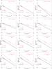Fig. 7 Excitation diagrams of shock and PDR model-predicted H2 line column density distributions as a function of upper energy level. The column density is normalized to the 1-0 S(1) H2 transition. Diamonds represent lines from v = 1 while the asterisks represent points from v > 1. The solid line is a best fit of the Boltzmann distribution to the v = 1 points, the slope represents the excitation temperature, Tex. Predictions of shock models from Shull & Hollenbach (1978) with shock speeds 6 km s-1 (top row) and 14 km s-1 (second row) and densities nH = 103 cm-3 (left), 104 cm-3 (middle), and 105 cm-3 (right). Predictions of PDR models from Black & van Dishoeck (1987) with Iuv = 100 − 104 and densities nH = 103 cm-3, 104 cm-3, and 105 cm-3, and are labeled with BvD.

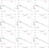Fig. 8 Excitation diagrams of observed H2 line column density distribution as a function of upper energy level. The column density is normalized to the 1-0 S(1) H2 transition. Diamonds represent lines from v = 1 while the asterisks represent points from v > 1. The solid line is a best fit of the Boltzmann distribution to the v = 1 points, the slope represents the excitation temperature, Tex. Each panel represents a different region, corresponding to the regions in Fig. 5. The error bars represent a standard deviation from the column density.

In order to directly compare the observed line ratios in NGC 253 to model predictions, we can use predicted line intensities for shock and PDR models and plot them on this diagnostic energy level diagram. Figure 7 presents the results from the Shull & Hollenbach (1978) shock models. These models calculate line intensities for shocks moving at 6, 10, and 14 km s^-1 for densities of 10³, 10⁴, 3   ×   10⁵ cm^-3. In most of the shock models of Fig. 7, the v > 1 lines (depicted as triangles) lie on or below the thermal distribution indicating subthermal excitation of the higher levels. The exceptions to this case are the higher velocity (10 − 14 km s^-1) shocks in very dense environments (n_H = 10⁵). However, the v > 1 lines have a shallower slope than the thermal distribution as shown by the dotted red line, indicating a higher excitation temperature for these transitions. In these high velocity, high density shocks, there are two different gas components (temperature slopes).

The bottom 6 panels of Fig. 7 displays the predicted line intensities from Sternberg & Dalgarno (1989), who model fluorescent excitation of H₂ in environments with n_H = 10³ − 10⁶ and χ = 10² and Black & van Dishoeck (1987) who model pure fluorescent excitation for a large range of the parameter space. We have chosen models 4, 6, 9, 17,19, and 20 spanning densities of n_H = 10² − 10⁴ cm^-3 and radiation intensities of χ = 10⁰ − 10⁴. In contrast to the shock models, the PDR models show the v > 1 lines lying high above the thermal distribution in almost all cases, since UV fluorescence populates levels from the top down, the highest energy levels get populated with higher probability compared to the thermalized case. In addition, the lines belonging to the v = 2 level share the same excitation temperature (same slope) as the v = 1 lines, only offset due to their higher upper energy level, unlike the shock models where there are two distinct excitation temperatures. This is the same for each v level, as shown in Black & van Dishoeck (1987). A general feature of the UV-excited models is that the rotational temperatures (i.e., the excitation temperature determined between different rotational levels within the same vibrational level) are the same in the various vibrational levels. In contrast, the vibrational temperature (i.e., the excitation temperature determined between different vibrational levels) is higher than the rotational temperature. The only exception to this pattern is the top-right panel of Fig. 9, showing a model with low radiation field but very high density. However, this density is only relevant for very dense clumps and the the bulk of the molecular gas in NGC 253 is at much lower densities.

Now that we have presented the shock and PDR models, we can compare them to the observational results seen in Fig. 8. In these plots, only the ( ≥ 2σ) H₂ line detections are included. Each panel of the figure represents the different regions shown in Fig. 1. In each region, Fig. 8 reveals the thermalized v = 1 lines of varying excitation temperatures. In addition, in all regions where v > 1 lines are detected, they lie above the thermal distribution. However, the case becomes ambiguous in regions where we cannot detect v > 1 lines, such as Regions 8 and 9. It is possible that in these regions shocks dominate and therefore the higher transitions are not being populated, or that in these regions, we lack the signal to noise to detect the lines above 2σ.

In both Region 1 and Region 3, the kinematic center, we detect two v = 2 lines and one v = 3 line. Although we only have two v = 2 lines, it is clear that they have a similar excitation temperature (slope) to the thermal distribution and do not represent a second hotter gas component. Thus, these lines clearly follow a PDR distribution. In addition, the v > 2 lines cannot be excited through shocks, so the presence of the 3-2 S(3) line also suggests fluorescent excitation. Using these criteria and the shock/PDR models as a guide, we can conclude that there is fluorescent excitation in Regions 1, 3, and 4 and most likely in Regions 2, 5 and 6. Since the signal-to-noise is too low in Regions 7 and 8, we cannot determine whether shock excitation or fluorescent excitation is the dominant heating mechanism in these regions. However, based on the integrated spectrum and Regions 1, 2, 3, and 4, it is clear that UV excitation in PDRs is the dominant mechanism for this galaxy, although shocks may dominate in some isolated areas.

7. Conclusion

From SINFONI observations, we determine the nature of the excitation of hot H₂ gas in NGC 253 using diagnostic emission lines. Specifically, we use the K band continuum as a tracer of the older stellar population, Brγ as a tracer of high-mass, young (O-type) star formation, [FeII] as a tracer of shocks, and PAHs as a tracer of slightly lower mass (B-type) star formation. Based on the Brγ and [FeII] emission line maps, we can interpret the H₂ excitation. We find that in most regions of NGC 253, excitation by UV photons in PDRs is the dominant mechanism. There are 3 regions where shock excitation may dominate, but these are small relatively isolated regions. Throughout the entire nuclear region of the galaxy, H₂ is being fluorescently excited.

We also present a diagnostic energy level diagram which robustly differentiates between shock and fluorescent excitation. By comparing the observed column densities of each line to the proposed PDR and shock models, it is clear that the NGC 253 H₂ is dominated by fluorescent excitation. A few of the bright H₂ regions may lack the signal-to-noise to resolve the higher energy transitions, or it is possible that in these isolated regions, shocks are the dominant mechanism. In addition, the PAH emission follows the same morphology as the H₂, adding further confidence that through NGC 253, the gas is undergoing fluoresce.

We determine that a maximum of 29% of the hot molecular gas is excited by shocks. Since we are only sensitive to the hottest H₂ gas, we are probing the surfaces of molecular clouds. Within the molecular clouds, where the bulk of the molecular gas is, the gas can have a different excitation mechanism.

Acknowledgments

We thank Lowell Tacconi-Garman for making his ISAAC 3.21 and 3.28 mu images available to us, and Susanne Brown for determining the calibration factors of these images.

References

All Tables

All Figures

Fig. 1 K band continuum map and H2 1-0 S(1) line map of NGC 253. The offset from the kinematic center at position $\mathrm{(}\mathit{\alpha ,\delta }{\mathrm{)}}_{\mathrm{2000}}\mathrm{=}\mathrm{(}{\mathrm{00}}^{\mathrm{h}}{\mathrm{47}}^{\mathrm{m}}\mathrm{33}\stackrel{\mathrm{s}}{.}\mathrm{14}\mathit{,}\mathrm{-}{\mathrm{25}}^{\mathrm{◦}}{\mathrm{17}}^{\mathrm{\prime }}\mathrm{17}\stackrel{\mathrm{″}}{.}\mathrm{52}\mathrm{)}$ is given on each axis. The contours represent 13 equally spaced levels with a maximum flux of 1.3 × 10-11 erg s-1 cm-2  μm-1 arcsec-2 and 5.4 × 10-15 erg s-1 cm-2 arcsec-2, for the K band continuum and H2 respectively. The white rectangular regions are H2 flux peaks, with the exception of Region 3, which is centered on the kinematic center. The blue “+” represents the kinematic center, the blue triangle represents X-1 and the blue diamond represents TH2.

In the text

Fig. 2 Brγ and [FeII]1.64 emission line map of NGC 253. The offset from the kinematic center at position $\mathrm{(}\mathit{\alpha ,\delta }{\mathrm{)}}_{\mathrm{2000}}\mathrm{=}\mathrm{(}{\mathrm{00}}^{\mathrm{h}}{\mathrm{47}}^{\mathrm{m}}\mathrm{33}\stackrel{\mathrm{s}}{.}\mathrm{14}\mathit{,}\mathrm{-}{\mathrm{25}}^{\mathrm{◦}}{\mathrm{17}}^{\mathrm{\prime }}\mathrm{17}\stackrel{\mathrm{″}}{.}\mathrm{52}\mathrm{)}$ is given on each axis. The contours represent 13 equally spaced levels with a maximum flux of 4.5 × 10-14 and 2.8 × 10-14 erg s-1 cm-2 arcsec-2 for Brγ and [FeII] respectively. The white rectangular regions are areas of concentrated H2 flux, with the exception of Region 3, which is centered on the kinematic center.

In the text

Fig. 3 K band spectra of H2 bright clumps. The integrated K band spectra, in the rest frame, integrated over the regions shown in Fig. 1. Vertical dotted lines are used to show dominant emission lines. The strongest OH lines have been marked in the spectrum of Region 1 with the red dot-dash line. The 12CO absorption bands are also visible at 2.294, 2.323, and 2.353 μm respectively. Region 2 is the K Continuum peak and hot spot, Region 3 is the kinematic nucleus, and Region 4 is the H2 emission peak.

In the text

Fig. 4 Stellar velocity field (left) with H2 1-0 S(1) velocity contours and H2 1-0 S(1) velocity map with contours (right). The contour levels are  − 75, − 50, − 30, − 10,0,10,30,50,75 km s-1. The color bar describes the H2 and stellar velocity in km s-1. On the right panel, the red circle represents the 3σ uncertainty for the center defined by Müller-Sánchez et al. (2010). The plus sign is the center of this circle, and the kinematic center. The diamond is TH2, the radio peak. The triangle is X-1, the X-ray peak. The square is the point of highest symmetry.

In the text

Fig. 5 The ratio of 2-1 S(1)/1-0 S(1) H2 lines with the Brγ line map over plotted in contours. The white rectangles are the same regions as defined in Fig. 1. The color bar values represent the value of the ratio. The offset from the kinematic center at position $\mathrm{(}\mathit{\alpha ,\delta }{\mathrm{)}}_{\mathrm{2000}}\mathrm{=}\mathrm{(}{\mathrm{00}}^{\mathrm{h}}{\mathrm{47}}^{\mathrm{m}}\mathrm{33}\stackrel{\mathrm{s}}{.}\mathrm{14}\mathit{,}\mathrm{-}{\mathrm{25}}^{\mathrm{◦}}\mathrm{17}\prime \mathrm{17}\stackrel{\mathrm{″}}{.}\mathrm{52}\mathrm{)}$ is given on each axis. Ratio values where the line flux of either transition is below 10% of the maximum flux of that line are masked.

In the text

Fig. 6 Top panels: PAH 3.28 μm continuum subtracted image from ISAAC. Left panel has H2 1-0 S(1) contours, middle panel has Brγ contours, right panel has [FeII]1.64 contours. The offset from the kinematic center at position $\mathrm{(}\mathit{\alpha ,\delta }{\mathrm{)}}_{\mathrm{2000}}\mathrm{=}\mathrm{(}{\mathrm{00}}^{\mathrm{h}}{\mathrm{47}}^{\mathrm{m}}\mathrm{33}\stackrel{\mathrm{s}}{.}\mathrm{14}\mathit{,}\mathrm{-}{\mathrm{25}}^{\mathrm{◦}}{\mathrm{17}}^{\mathrm{\prime }}\mathrm{17}\stackrel{\mathrm{″}}{.}\mathrm{52}\mathrm{)}$ is given on each axis. The kinematic center is from Müller-Sánchez et al. (2010). Bottom panels: pixel-pixel plots of PAH flux vs. H2 flux (left), Brγ flux (center), and [FeII] flux (right). The pixels of the ISAAC PAH observations were rebinned to match those of the SINFONI observations.

In the text

Fig. 7 Excitation diagrams of shock and PDR model-predicted H2 line column density distributions as a function of upper energy level. The column density is normalized to the 1-0 S(1) H2 transition. Diamonds represent lines from v = 1 while the asterisks represent points from v > 1. The solid line is a best fit of the Boltzmann distribution to the v = 1 points, the slope represents the excitation temperature, Tex. Predictions of shock models from Shull & Hollenbach (1978) with shock speeds 6 km s-1 (top row) and 14 km s-1 (second row) and densities nH = 103 cm-3 (left), 104 cm-3 (middle), and 105 cm-3 (right). Predictions of PDR models from Black & van Dishoeck (1987) with Iuv = 100 − 104 and densities nH = 103 cm-3, 104 cm-3, and 105 cm-3, and are labeled with BvD.

In the text

Fig. 8 Excitation diagrams of observed H2 line column density distribution as a function of upper energy level. The column density is normalized to the 1-0 S(1) H2 transition. Diamonds represent lines from v = 1 while the asterisks represent points from v > 1. The solid line is a best fit of the Boltzmann distribution to the v = 1 points, the slope represents the excitation temperature, Tex. Each panel represents a different region, corresponding to the regions in Fig. 5. The error bars represent a standard deviation from the column density.

In the text

References

- Alonso-Herrero, A., Rieke, G. H., Rieke, M. J., & Kelly, D. M. 2003, AJ, 125, 1210 [NASA ADS] [CrossRef] [Google Scholar]
- Bakes, E. L. O., & Tielens, A. G. G. M. 1994, ApJ, 427, 822 [NASA ADS] [CrossRef] [Google Scholar]
- Black, J. H., & van Dishoeck, E. F. 1987, ApJ, 322, 412 [NASA ADS] [CrossRef] [Google Scholar]
- Cappellari, M., & Copin, Y. 2003, MNRAS, 342, 345 [NASA ADS] [CrossRef] [Google Scholar]
- Cappellari, M., & Emsellem, E. 2004, PASP, 116, 138 [NASA ADS] [CrossRef] [Google Scholar]
- Demoulin, M. H., & Burbidge, E. M. 1970, ApJ, 159, 799 [NASA ADS] [CrossRef] [Google Scholar]
- Engelbracht, C. W., Rieke, M. J., Rieke, G. H., Kelly, D. M., & Achtermann, J. M. 1998, ApJ, 505, 639 [NASA ADS] [CrossRef] [Google Scholar]
- Fabbiano, G., & Trinchieri, G. 1984, ApJ, 286, 491 [NASA ADS] [CrossRef] [Google Scholar]
- Fernández-Ontiveros, J. A., Prieto, M. A., & Acosta-Pulido, J. A. 2009, MNRAS, 392, L16 [NASA ADS] [CrossRef] [Google Scholar]
- Forbes, D. A., Ward, M. J., & Depoy, D. L. 1991, ApJ, 380, L63 [NASA ADS] [CrossRef] [Google Scholar]
- Forbes, D. A., Ward, M. J., Rotaciuc, V., et al. 1993, ApJ, 406, L11 [NASA ADS] [CrossRef] [Google Scholar]
- Forbes, D. A., Polehampton, E., Stevens, I. R., Brodie, J. P., & Ward, M. J. 2000, MNRAS, 312, 689 [NASA ADS] [CrossRef] [Google Scholar]
- García-Burillo, S., Martín-Pintado, J., Fuente, A., & Neri, R. 2000, A&A, 355, 499 [NASA ADS] [Google Scholar]
- Grimm, H.-J., Gilfanov, M., & Sunyaev, R. 2003, MNRAS, 339, 793 [NASA ADS] [CrossRef] [Google Scholar]
- Harrison, A., Puxley, P., Russell, A., & Brand, P. 1998, MNRAS, 297, 624 [NASA ADS] [CrossRef] [Google Scholar]
- Israel, F. P., Hawarden, T. G., Wade, R., Geballe, T. R., & van Dishoeck, E. F. 1989, MNRAS, 236, 89 [NASA ADS] [Google Scholar]
- Jones, A. P., Tielens, A. G. G. M., Hollenbach, D. J., & McKee, C. F. 1994, ApJ, 433, 797 [NASA ADS] [CrossRef] [Google Scholar]
- Kornei, K. A., & McCrady, N. 2009, ApJ, 697, 1180 [NASA ADS] [CrossRef] [Google Scholar]
- Luhman, M. L., Jaffe, D. T., Keller, L. D., & Pak, S. 1994, ApJ, 436, L185 [NASA ADS] [CrossRef] [Google Scholar]
- Martín, S., Mauersberger, R., Martín-Pintado, J., Henkel, C., & García-Burillo, S. 2006, ApJS, 164, 450 [NASA ADS] [CrossRef] [Google Scholar]
- Martín, S., Martín-Pintado, J., & Mauersberger, R. 2009a, ApJ, 694, 610 [NASA ADS] [CrossRef] [Google Scholar]
- Martín, S., Martín-Pintado, J., & Viti, S. 2009b, ApJ, 706, 1323 [NASA ADS] [CrossRef] [Google Scholar]
- McCarthy, P. J., van Breugel, W., & Heckman, T. 1987, AJ, 93, 264 [NASA ADS] [CrossRef] [Google Scholar]
- Mouri, H., Kawara, K., & Taniguchi, Y. 2000, ApJ, 528, 186 [NASA ADS] [CrossRef] [Google Scholar]
- Müller-Sánchez, F., González-Martín, O., Fernández-Ontiveros, J. A., Acosta-Pulido, J. A., & Prieto, M. A. 2010, ApJ, 716, 1166 [NASA ADS] [CrossRef] [Google Scholar]
- Rekola, R., Richer, M. G., McCall, M. L., et al. 2005, MNRAS, 361, 330 [NASA ADS] [CrossRef] [Google Scholar]
- Rieke, G. H., Lebofsky, M. J., Thompson, R. I., Low, F. J., & Tokunaga, A. T. 1980, ApJ, 238, 24 [NASA ADS] [CrossRef] [Google Scholar]
- Rieke, G. H., Lebofsky, M. J., & Walker, C. E. 1988, ApJ, 325, 679 [NASA ADS] [CrossRef] [Google Scholar]
- Rosenberg, M. J. F., van der Werf, P. P., & Israel, F. P. 2012, A&A, 540, A116 [NASA ADS] [CrossRef] [EDP Sciences] [Google Scholar]
- Sakamoto, K., Mao, R.-Q., Matsushita, S., et al. 2011, ApJ, 735, 19 [NASA ADS] [CrossRef] [Google Scholar]
- Shull, J. M., & Hollenbach, D. J. 1978, ApJ, 220, 525 [NASA ADS] [CrossRef] [Google Scholar]
- Sternberg, A., & Dalgarno, A. 1989, ApJ, 338, 197 [NASA ADS] [CrossRef] [Google Scholar]
- Turner, J. L., & Ho, P. T. P. 1985, ApJ, 299, L77 [NASA ADS] [CrossRef] [Google Scholar]
- Ulrich, M.-H. 1978, ApJ, 219, 424 [NASA ADS] [CrossRef] [Google Scholar]
- Ulvestad, J. S., & Antonucci, R. R. J. 1997, ApJ, 488, 621 [NASA ADS] [CrossRef] [Google Scholar]
- Watson, A. M., Gallagher, III, J. S., Holtzman, J. A., et al. 1996, AJ, 112, 534 [NASA ADS] [CrossRef] [Google Scholar]
- Weaver, K. A., Heckman, T. M., Strickland, D. K., & Dahlem, M. 2002, ApJ, 576, L19 [NASA ADS] [CrossRef] [Google Scholar]
- Westmoquette, M. S., Smith, L. J., & Gallagher, III, J. S. 2011, MNRAS, 414, 3719 [NASA ADS] [CrossRef] [Google Scholar]
- Wolniewicz, L., Simbotin, I., & Dalgarno, A. 1998, ApJS, 115, 293 [NASA ADS] [CrossRef] [Google Scholar]
All Tables
Integrated fluxes for selected regions and over the full map of all detected H2 transitions.
Calculated supernova rates for each region and the integrated galaxy based on [FeII] luminosity.