| Issue |
A&A
Volume 550, February 2013
|
|
|---|---|---|
| Article Number | A120 | |
| Number of page(s) | 20 | |
| Section | Catalogs and data | |
| DOI | https://doi.org/10.1051/0004-6361/201220184 | |
| Published online | 05 February 2013 | |
Improved variability classification of CoRoT targets with Giraffe spectra⋆,⋆⋆
1 Dpt. de Inteligencia Artificial, UNED, Juan del Rosal, 16, 28040 Madrid, Spain
e-mail: This email address is being protected from spambots. You need JavaScript enabled to view it.
2 Instituut voor Sterrenkunde, KU Leuven, Celestijnenlaan 200D, 3001 Leuven, Belgium
e-mail: This email address is being protected from spambots. You need JavaScript enabled to view it.
3 LESIA, UMR 8109 du CNRS, Observatoire de Paris, UPMC, Univ. Paris Diderot, 5 place Jules Janssen, 92195 Meudon Cedex, France
4 Dept. of Construction and Industrial Manufacturing, University of Oviedo, 33203 Gijón, Spain
5 Department of Mechanical Engineering, University of La Rioja, c/ Luis de Ulloa, 20, 26004 Logroño, Spain
6 PMQ Research Team; ETSII; Universidad Politécnica de Madrid, José Gutiérrez Abascal 2, 28016 Madrid, Spain
e-mail: This email address is being protected from spambots. You need JavaScript enabled to view it.
7 Department of Astrophysics, IMAPP, Radboud University Nijmegen, PO Box 9010, 6500 GL Nijmegen, The Netherlands
Received: 7 August 2012
Accepted: 16 December 2012
Abstract
Aims. We present an improved method for automated stellar variability classification, using fundamental parameters derived from high resolution spectra, with the goal to improve the variability classification obtained using information derived from CoRoT light curves only. Although we focus on Giraffe spectra and CoRoT light curves in this work, the methods are much more widely applicable.
Methods. In order to improve the variability classification obtained from the photometric time series, only rough estimates of the stellar physical parameters (Teff and log (g)) are needed because most variability types that overlap in the space of time series parameters, are well separated in the space of physical parameters (e.g. γ Dor/SPB or δ Sct/β Cep). In this work, several state-of-the-art machine learning techniques are combined to estimate these fundamental parameters from high resolution Giraffe spectra. Next, these parameters are used in a multi-stage Gaussian-Mixture classifier to perform an improved supervised variability classification of CoRoT light curves. The variability classifier can be used independently of the regression module that estimates the physical parameters, so that non-spectroscopic estimates derived e.g. from photometric colour indices can be used instead.
Results. Teff and log (g) are derived from Giraffe spectra, for 6832 CoRoT targets. The use of those parameters in addition to information extracted from the CoRoT light curves, significantly improves the results of our previous automated stellar variability classification. Several new pulsating stars are identified with high confidence levels, including hot pulsators such as SPB and β Cep, and several γ Dor-δ Sct hybrids. From our samples of new γ Dor and δ Sct stars, we find strong indications that the instability domains for both types of pulsators are larger than previously thought.
Key words: stars: variables: general / stars: oscillations / techniques: spectroscopic / stars: fundamental parameters / methods: statistical / methods: data analysis
The CoRoT space mission, launched on 27 December 2006, has been developed and is operated by CNES, with the contribution of Austria, Belgium, Brazil, ESA (RSSD and Science Programmes), Germany, and Spain.
Full Table 2 is only available in electronic form at the CDS via anonymous ftp to cdsarc.u-strasbg.fr (130.79.128.5) or via http://cdsarc.u-strasbg.fr/viz-bin/qcat?J/A+A/550/A120
© ESO, 2013
1. Introduction
The CoRoT space mission (Auvergne et al. 2009) has been delivering stellar light curves of excellent quality in the past 5 years for thousands of faint (11 < V < 16.5) stars, as a by-product of the search for exoplanets using the occultation method. The majority of the observed targets has not been studied before, implying that amongst the thousands of targets, plenty of new variable stars are present. Identifying them in the CoRoT database requires the use of automated light curve analysis and classification methods, given the very large number of objects. In Debosscher et al. (2009), an automated supervised classification (CVC: CoRoT variability classifier) was described, using classification attributes derived from the CoRoT light curves only. While the methods allowed the efficient detection of members of several known stellar variability classes, using classification information derived from light curves in a single passband is not sufficient to distinguish all variability types. In this paper, we describe the use of high resolution spectra obtained with the Giraffe spectrograph installed at the VLT in Chile, to improve our variability classification.
The advent of automated spectral surveys (e.g. the Sloan Digital Sky Survey (Eisenstein et al. 2011), RAVE (Siebert et al. 2011), or the Gaia-ESO survey Gilmore et al. 2012) has raised the necessity of automated methods for the inference of physical parameters from spectra. This has been tackled in the past with a variety of methods, including machine learning techniques like artificial neural networks (Bailer-Jones 2000; Allende Prieto et al. 2000) or oblique k-d decision trees (Kordopatis et al. 2011), maximum likelihood techniques (Soubiran et al. 1998;Lee et al. 2008; Jofré et al. 2010), or statistical modelling techniques (Recio-Blanco et al. 2006; Bailer-Jones 2010). A recent contextual survey of existing techniques can be found in Bijaoui et al. (2010). These works were mostly optimised for specific temperature or spectral type ranges and for various resolutions and spectral ranges not exactly matching the needs posed by the Giraffe spectra of CoRoT targets treated here. All of them can be modified and adapted for these needs, but we prefered to explore alternatives to the forementioned approaches as part of a broader study of parameter estimation of stellar atmospheres. In this work, we analyse the performance of a projection scheme based on independent component analysis (ICA) combined with support vector machines, and compare the results obtained by training the models with synthetic spectra, with those obtained from empirical spectral libraries. However, it is not the purpose of this work to focus on the problem of stellar parameter estimation and the evaluation of the various alternatives, but to advance in the improvement of the classification of variability, and in the understanding of the main characteristics of multiperiodic variability types.
In Sect. 2, we describe the target selection procedure we used, and provide information on the Giraffe observations. Sections 3 describes the derivation of fundamental astrophysical parameters Teff and log (g) from the obtained spectra, using a combination of machine learning techniques, including an evaluation of the quality of the predictions thus obtained. Next, the inclusion of the derived parameters as complementary attributes in the supervised classification methods is described in Sect. 4, as well as the results of the application to the subsample of 6832 stars of the CoRoT database for which we obtained Giraffe spectra. A comparison is made between the old (without spectral information) and new classifications, in terms of numbers of good candidate pulsators for the relevant classes. We present some new candidate pulsating stars (δ Sct, γ Dor, slowly pulsating B (SPB)-stars, β Cep and hybrid δ Sct-γ Dor), which are now much more confidently classified. For the samples of new δ Sct and γ Dor candidates, we investigated correlations between light curve parameters, log (g) and Teff, and made a comparison with results from the Kepler space mission (Sect. 5). Finally, we end with our conclusions in Sect. 6 and give outlines for future work and improvements.
2. Giraffe observations and target selection
We obtained observations with the Giraffe multi-object spectrograph installed at VLT at ESO in Chile (Run ID 082.D-0839, 083.D-0479, 085.D-0829 and 086.D-0212; PI Neiner). We used two low resolution MEDUSA settings: LR2 and LR6. LR2 is centered at 4272 Å and covers the wavelength range from 3964 to 4567 Å; LR6 is centered at 6822 Å and covers the range from 6438 to 7184 Å. These settings correspond to a spectral resolving power of 6400 and 8600, respectively.
We observed variable targets of the IR1, LRA1, LRC1, LRC2 and LRA2 CoRoT fields in about 82 hours of telescope acquisition time (54.5 h in LR2 and 27.3 h in LR6). This corresponds to the observation of 216 Giraffe fields of about 125 stars each, i.e. about 27000 observed spectra of 8062 different stars. We also pointed about 5 fibers per observed Giraffe field on sky regions. Only 6832 of these stars have spectra in the LR2 setting. The derivation of stellar parameters described in Sect. 3 and the subsequent analysis of variability described in Sect. 4 apply only to this set of 6832 CoRoT targets.
Standard calibrations were obtained together with the stellar observations. The data were reduced using the ESO Giraffe reduction pipeline and EsoRex scripts with parameters tuned to extract the data in the best way on average for all targets. Considering that the observed fields contain at the same time hot and cool stars of various magnitudes, these parameters are not necessarily optimized for all targets.
The CVC was applied to all lightcurves obtained in the exoplanet fields of CoRoT to obtain a first classification of the stars and their level of variability. The most variable targets were then selected from this list to be observed with Giraffe. These targets were prioritized according to their variability (the higher the variability level, the higher the priority) and to their rarety (e.g. RR Lyrae stars are rather rare and were thus given a higher priority ranking).
Each 1.3 deg2 CoRoT CCD can be covered by 9 circular 25 arcmin Giraffe fields. Stars falling between the circular Giraffe fields could not be observed. In each Giraffe field, one VLT guide star has to be selected and is used to first point the telescope, for accurate tracking, and for the active control of the telescope mirrors. The VLT arm to this guide star blocks part of the Giraffe field and forbids the allocation of Giraffe fibers to the targets behind this arm. To limit the impact of the arm, guide stars were chosen as close to the edge of the field as possible. In addition, Giraffe fibers have a diameter of 1.2 arcsec and should be separated by at least 11 arcsec from one another. Therefore, when two stars were closer than 12.2 arcsec from each other, only one of them could be observed. Finally, the positioning of the Giraffe fibers by the positioner robot is restricted (e.g. by the fiber length or too much fiber crossing), which also led us to discard some targets. In this complete fiber allocation procedure, the targets with highest ranking were always given priority.
3. Determination of the astrophysical parameters of CoRoT targets
In the following, we will describe the regression models developed in order to complement the time series attributes used in Debosscher et al. (2009) for the classification of stars into variability types. Our main objective here is to provide a temperature estimate in order to separate variability types that overlap in the space of attributes used previously for the classification of CoRoT time series. In this sense, the temperature predictions need not be extremely precise because the temperature domains of these overlapping classes are well separated (see Sect. 4).
Using effective temperatures to improve the classifier has the advantage that the improved classification model can be applied even if no spectrum is available, as long as we have a Teff estimate. These estimates can be available from the fitting of photometric spectral energy distributions (SEDs), or from narrow band multi-colour photometry.
We construct the regression models using synthetic spectral libraries covering a wide range of temperatures and gravities. In particular, we use the Kurucz models as provided by the BLUERED library (Bertone et al. 2008) and the TLUSTY grids of models (Hubeny & Lanz 1995)1 with metallicities Z/Z⊙ = 0.5, 1, and 2.
In order to check the validity of the regression models, we use two empirical datasets. The ELODIE library (Prugniel & Soubiran 2001, 2004) contains 1962 spectra, and effective temperatures, surface gravities, and metallicities for 1388 stars. In the validation of the regression models with ELODIE spectra we use the R = 10 000 versions of the spectra where available or else, we degrade the resolution down to this value. Also, we use the PASTEL dataset (Soubiran et al. 2010) to compare the distribution of predictions in the Teff – log (g) space by our regression models with that of an independent sample.
3.1. Data pre-processing and dimensionality reduction
The first stage in the analysis of regression models for the determination of the effective temperatures and gravities of CoRoT targets is the homogenisation of the spectra. This involves sky subtraction, the correction for potential Doppler shifts, the trimming and interpolation of the spectra to introduce a constant wavelength scale, cosmic ray elimination, continuum subtraction and normalisation.
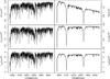 |
Fig. 1 Giraffe spectra of the first two CoRoT targets in the catalog (top). In the middle row, we show the same spectra after continuum subtraction (Fcs(λ)), and the lower row shows the spectra after rescaling (subtraction of the minimum flux and normalisation to unit area; Fscl(λ)). |
The sky was removed from each spectrum by subtracting averaged sky exposures for each Giraffe field separately, taking the observing times into account. Sky correction is especially important for some fainter targets, observed during the presence of moonlight. In fact, for the faintest targets, the contribution of the flux originating from the sky can be as high as the stellar flux. Not correcting for this, these targets would all appear to be of solar spectral type and be assigned the wrong Teff and log (g) values. This would then translate into degraded classification performance when combining both light curve and spectral information.
The next stage in the pre-processing consists of the correction of Doppler shifts of the Giraffe spectra. We do not interpolate the spectra and thus, correct for Doppler shifts only up to the spectral precision of one pixel (0.2 Å or 15 km s-1). An estimate of the radial velocity of the star was obtained by cross-correlating the spectrum with a series of theoretical templates downgraded to the LR2 spectral resolution and sampling. No binary mask was used in the cross-correlation.
After correcting the observed spectra for potential Doppler shifts, all the spectra (i.e. both synthetic and empirical) are interpolated to a common wavelength scale. In order to do so, we look for the interval of wavelengths covered by all observed spectra after the Doppler corrections. This way no extrapolation is needed outside of the observed spectral range. The final range of wavelengths used in the regression starts at 396.02 and ends at 456.40 nm. We have tested the LR2 and LR6 spectra separately and in conjunction. The results indicate that the LR6 spectra do not add significant information to that already contained in the LR2 data (as shown further below).
A flux value is flagged as being affected by a cosmic ray if it exceeds 5 median absolute deviations with respect to the median computed from 50 adjacent values on each side. Cosmic rays are masked and interpolated using a polynomial of order 3 from the neighbouring regions of the spectrum.
The observed spectra are then continuum subtracted using a unique third order polynomial fitted to the flux values between the 80-th and 90-th percentiles of the flux distribution. In the calculation of the percentiles we remove the following wavelength ranges with potentially deep absorption lines: 396.02−401.0, 406.02−416.0, 426.02−442.0, and 456.02−456.4 nm. This effectively avoids most prominent absorption lines. In the case of the synthetic spectra, the polynomial is fitted using the same intervals but percentiles 90 and 100.
Finally, the spectra (both synthetic and empirical) are rescaled such that the area under the spectrum equals unity, and the minimum value is zero. The results of the continuum subtraction and subsequent rescaling are shown in Fig. 1 for the first two CoRoT spectra in the catalog.
Rescaling or standarisation of the input variables is common practice in statistical learning (see for example the classical text book by Bishop 1995). There are many ways in which an input vector can be normalised/rescaled. It is not the aim of this work to assess the relative merits of the various alternatives. We have selected areal normalisation to avoid division by small numbers in low signal-to-noise ratio spectra.
Instrumental signatures can be of two types: additive or multiplicative. Both should be removed in the reduction process, but for obvious reasons there could remain residual signatures. Our normalisation methods result in the same normalised spectrum when applied to data without these residual signatures, to data affected by additive biases, and by multiplicative biases that do not depend on wavelength. Wavelength dependent multiplicative biases are not removed by our normalisation process and thus, the resulting normalised spectrum differs from that of the unbiased spectrum. On the other hand, the classical division by the continuum removes multiplicative biases of any kind, but the normalised spectrum is not invariant under additive biases, regardless of whether they are wavelength dependent or not.
As a result of the previous homogenisation process, the spectra or input patterns consist of 3036 variables (the flux measurements at each wavelength), while the number of patterns (spectra) available for training the regression models is much lower (see Fig. 2). The high dimensionality of the space of independent variables (also known as feature space dimensionality, equal to 3036) implies a need for correspondingly large training sets to ensure the availability of examples sufficiently close to the input pattern. The number of examples needed to maintain a constant density of examples per unit of hyper-volume in the feature space increases exponentially with the dimensionality of this space. This is the so-called curse of dimensionality problem in statistical learning. In order to overcome this difficulty, a reduction of dimensionality was performed as a way to identify global features and trends present in the pattern sets (Marshall 2002). There are many possibilities for doing this (Fodor & Kamath 2002). In this work we have preferred to tackle the problem by projecting the original spectra in the space of independent components using independent component analysis (ICA, Cao et al. 2003) because this results in features which are mutually statistically independent, and not only uncorrelated features as in the case of Principal Components Analysis (PCA). Statistical independence makes ICA a powerful and robust projection technique in the analysis of spectra in several areas of research (Daszykowski 2007; Suzuki & Sugillama 2011).
The dimensionality of the projection space is determined using the cross-validation technique, whereby the full dataset is divided into n blocks, and (n − 1) are used for the determination of the independent components, and the remaining spectra are used for the evaluation of the results. By repeating this procedure with the n blocks that can be chosen for evaluation, we can compute an estimate of the reconstruction error that will be obtained when all the spectra are used to define the independent components. In this analysis we have adopted the value n = 10 in the application of the cross-validation method for the determination of the independent components from the synthetic spectra.
We assess the reconstruction error projecting the original synthetic spectra in the Kurucz and TLUSTY libraries into the new basis of independent components, retaining the contribution of the first 20 components, and transforming back into the original space of spectra. We subsequently compare the original and recovered spectra, and compute the reconstruction error as the ratio of the root-mean-square error (RMSE) of the reconstruction to the sum of flux values in the original. In practice, we find that the median reconstruction error computed from n = 10 blocks is as low as 8.5% with only 2 independent components and decreases to 3.5% for 20 independent components. The standard deviation of this estimate (obtained from the sample of 10 median errors corresponding to the ten blocks used for evaluation) is consistently around 0.5% for data compressions above 5 independent components. Therefore, the final accuracy of the reconstruction error can be estimated as 3.5 ± 0.5% for the adopted 20 independent components. Anyhow, it is convenient to keep in mind that low reconstruction errors are desirable in any data compression approach that aims to alleviate the dimensionality problem, but it is in principle possible to find problems where a very small number of independent components characterised by large reconstruction errors are sufficient for optimal classification/regression if these components preserve the essential information needed for these tasks.
In the following we will describe the regression models based on Support Vector Machines (Vapnik 1995; Cortes & Vapnik 1995) applied to the ICA projection of the observed spectra. Two alternative approximations to the regression problem were tested for comparison: Kernel Partial Least Squares (Rosipal et al. 2001) and k-nearest neighbours (Cover & Hart 1967). The three alternatives were tested in combination with ICA, PCA (Principal Component Analysis) and Diffusion Maps (Coifman & Lafon 2006). Here we only report on the final choice made based on the internal prediction errors and the external validation with ELODIE and PASTEL data.
Global validation errors (mean absolute and root mean square error) for the ELODIE dataset obtained by predicting the values of Teff and log (g) using only the LR2 range, only the LR6 range, and the combination of the LR2 and LR6 wavelength ranges.
3.2. Determination of the effective temperature
It is important to remark that regression models are sensitive to the density of examples in the different regions of parameter space. In our case, the two synthetic libraries (Kurucz and TLUSTY) show very different densities of examples per effective temperature bin as shown in Fig. 2 and this results in the so-called “imbalanced learning problem”.
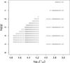 |
Fig. 2 Coverage in parameter space of the training sets used to construct the regression models. Crosses correspond to the Kurucz models and circles to the TLUSTY grid of models. |
Extensive analysis of the prediction accuracy in a wide range of settings resulted in the proposal of a multi-stage regression approach with specialised modules trained with sets of examples that are homogeneous in the space of parameters (Japkowicz & Stephen 2002). The forementioned analysis comprised the study of the prediction errors of regression modules specialised in different temperature and gravity ranges, assessed both with 10-fold cross-validation experiments and with the external validation made possible by the ELODIE collection of spectra. The cross-validation experiments consist in training the regression model with a certain fraction of the training set (e.g., a fraction of the complete set of the Kurucz+TLUSTY synthetic spectra), and assessing the model validity with the remaining fraction. External validation consists in training the regression model with a given training set (e.g., the complete set of Kurucz+TLUSTY synthetic spectra) and validating the model with an entirely independent dataset, for example the ELODIE dataset.
In the proposed multi-stage approach, we first classify Giraffe spectra into three broad categories: stars with Teff below 10 000 K, with Teff between 10 000 and 15 000 K, and finally, stars with Teff above 15 000 K. Depending on the category assigned in this initial pre-classification stage, a specialised Support Vector Machine (SVM) regression module is applied, trained only with models in that temperature range. The pre-classification is carried out with a boosting combination of artificial neural networks (ANN) and random forests (RF) trained with the entire set of synthetic spectra (Kurucz and TLUSTY). For a given Giraffe input spectrum, we obtain two temperature range predictions from the neural network (a multi-layer perceptron with three layers, 12 neurons in the hidden layer, and three binary output neurons, one for each temperature range) and the random forest (independent trees built from 500 bootstrap samples; each tree is trained with a subset of the complete set of fluxes (Ntot) of size  ). In addition to the two classifiers, we use a unique SVM model trained with spectra from the Kurucz model grid with Teff ≤ 10 000 K, and from the entire TLUSTY model grid. This SVM model predicts Teff and not only the temperature range. The temperature range assigned is deduced from the outcome of the three models (the ANN and RF classifiers and the SVM Teff prediction). If two out of the three predictions assign the first or third temperature ranges (below 10 000 K and above 15 000 K respectively), the category is straightforwardly assigned. Otherwise, the intermediate temperature range (between 10 000 and 15 000 K) is assumed.
Once the spectrum has been categorised, we apply i) an SVM model trained only with Kurucz synthetic spectra of effective temperatures below 10 000 K to stars in the first group; or ii) an SVM model trained with TLUSTY spectra of temperatures above 15 000 K to stars in the third category. Otherwise, we assign a weighted average of the predictions produced by both classifiers to stars in the intermediate range of temperatures. The average is weighted by the inverse distance of the two Teff predictions to the nearest interval boundary (10 000 or 15 000 K). The SVM models parameters (kernel size and noise contribution) are derived by minimising the Teff estimation errors for a validation set made up of ELODIE spectra in the corresponding temperature range. In the following, we will refer to this multi-stage model trained with synthetic spectra as the KT model (Kurucz-TLUSTY model).
This multi-stage approach implicitly assumes that the Kurucz family of models is a valid approximation to stellar spectra below 10 000 K and that the TLUSTY grid is valid above 15 000 K. There is no region of parameter space where the two families are used simultaneously to define the mapping between spectra and physical parameters via the training set. In the intermediate region between 10 000 and 15 000 K, an implicit interpolation is used between the mappings in the boundary regions. This is the best solution found, as evaluated from the validation with cross-validation experiments and the independent ELODIE dataset. Unfortunately, it is far from optimal. The ideal case would be a unique model family with a validity range spanning the entire range of expected physical parameters.
Table 1 shows a summary of the prediction errors for the spectra in the ELODIE catalog obtained using only the LR2 spectra, only the LR6 spectra or the combination of both. Since according to it, using only the LR2 spectra results in smaller errors, in the following we will concentrate on the results obtained with the LR2 spectra. The use of the ELODIE dataset as independent validation set in the generation of Table 1 implicitly gives a higher weight to the parameter ranges with overdensities in the ELODIE parameter space (i.e., Main Sequence stars between 5000 and 8000 K). The values included in Table 1 are global average errors, not restricted to examples in any temperature or gravity range.
The RMSE of the KT model predictions for the ELODIE dataset are 410 K for stars with Teff< 10 000 K and 4157 K for ELODIE stars with Teff> 15 000 K. The factor ten difference in the RMSEs of the two temperature regimes is mainly due to the very low density of examples per Teff interval above 10 000 K, and to the intrinsic degeneracy in the mapping, that translates very similar spectra into largely different effective temperatures in the high temperature regime. Figure 3 shows these degeneracies for four values of the stellar parameters. It represents the coverage of the parameter space conveyed by the ELODIE database. The colour code represents the difference between the reference spectrum (described by the values of Teff and log (g) included in each panel) and the rest of spectra in the ELODIE database as the area of the (absolute value of the) difference spectrum (it has to be recalled that the area of the spectra have been normalised to 1 as described above).
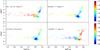 |
Fig. 3 Differences between four selected ELODIE spectra (indexed by the stellar parameters shown in each panel) and the ELODIE spectral collection. The panels show an approximation to the expected degeneracies in the mapping between spectra and physical parameters. The colour code represents the area of the (absolute value of the) difference between two pairs of spectra, where each spectrum has been normalised to area 1, as described in the text. |
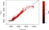 |
Fig. 4 Comparison of the effective temperatures assigned in the ELODIE spectral compilation and those predicted for the ELODIE dataset with Teff< 10 000 K by the non linear SVM model trained with Kurucz spectra with Teff< 10 000 K. The colour code reflects the log (g) value assigned in the ELODIE catalog. |
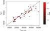 |
Fig. 5 Comparison of the effective temperatures assigned in the ELODIE spectral compilation and those predicted for the ELODIE dataset with Teff> 15 000 K by the non-linear SVM model trained with TLUSTY models. The colour code reflects the log (g) value assigned in the ELODIE catalog. |
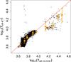 |
Fig. 6 Comparison of the Teff predictions by the ELODIE model (x axis) and the KT model (y axis). The median values in bins 0.1 dex wide defined in the x axis are shown in orange, and the median absolute deviations (MAD) are also shown as error bars. |
Figures 4, 5 show the distribution of errors when the KT module is applied to ELODIE spectra in the corresponding domains of applicability. We see how there is a systematic trend to overestimate Teff around 8000 K and to underestimate it above 9000 K. This trend is absent from the internal validation of the models (i.e., the assessment of the errors with Kurucz-TLUSTY spectra not used for training), and therefore we interpret this bias as the result of systematic differences between synthetic and observed spectra. We have found ways to correct for this bias, including a combination of models specialised in subdivisions of the full range of temperatures below 10 000 K or above 15 000 K. Unfortunately, these specialised models require additional preclassification stages to decide to what temperature sub-range a given spectrum pertains, and induce unwanted gaps in the distribution of Teff predictions for the CoRoT spectra.
We have checked for the dependence of error estimates with the signal-to-noise ratio of the ELODIE spectra. We find no systematic trend down to the lowest value of the signal-to-noise ratio in the ELODIE dataset (35, measured at 5500 Å and R = 42 000).
In all comparisons between ELODIE values of the physical parameters and the predictions from our regression models shown in this paper, it should be kept in mind that the ELODIE spectra cover a much wider spectral range (400−680 nm) than our observations and thus, have many more spectral lines available for diagnosing Teff and log (g).
The values of the RMSE quoted above may be slightly overfitted because the SVM kernel parameters (kernel size and noise contribution) were determined by minimising the prediction error for the ELODIE dataset. In any case, this is to be preferred to the internal cross-validation determination of these parameters based only on the Kurucz or TLUSTY datasets. The RMSEs obtained in the internal cross-validation of the models can be as low as a few Kelvin below 10 000 K, and a few tens of Kelvin for hotter stars, but these overfitted models result in very poor performances when applied to real collections of spectra such as the ELODIE dataset.
An analysis of the relative benefits of the various approaches to handling varying signal-to-noise ratios (like the noisification of the training set or the denoisification of the spectra) will be addressed in a subsequent paper.
For the sake of comparison, we constructed a multi-stage module (hereafter, the ELODIE model) entirely equivalent to the one described in the previous paragraphs but trained with ELODIE spectra in the same temperature ranges defined above. That is, one pre-classifier based on a combination of neural networks, random forests and SVMs, trained with all ELODIE spectra, and two specific regression modules based on SVMs and trained with ELODIE spectra with temperatures below 10 000 K and above 15 000 K respectively. In this case, the SVM Gaussian kernel parameters were determined by minimising the prediction error of an SVM model trained on 2/3 of the ELODIE dataset (obtained through random sampling) when applied to a validation set consisting of the remaining 1/3 of stars.
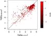 |
Fig. 7 Prediction accuracy of the regression model for gravity when applied to the ELODIE dataset. The y-axis represents the predictions from the regression model and the x-axis represents the log (g) values tabulated in the ELODIE catalog. The colour code represents the [Fe/H] values taken from the same catalog. |
We use both model predictions (KT and ELODIE) for the classification of CoRoT targets into variability types described in Sect. 4. In Fig. 6, we show a comparison of the prediction for the CoRoT dataset by the two regression models, with the values of the median and median absolute deviation (MAD) of the temperatures in (0.1 dex wide) bins of ELODIE effective temperatures (x-axis), superimposed as orange error bars. We see that below 10 000 K the difference between these median values is always below 0.03 dex, and the MAD reaches a maximum value of 0.05 around log (Teff) = 3.7.
There is a group of 139 spectra (1.3% of the total number of LR2 spectra) where the ELODIE model predictions are systematically above log (Teff) = 4.4 while the KT model predicts temperatures below log (Teff) = 3.9. We have visually inspected these spectra and the vast majority correspond to spectra of cool stars with low signal-to-noise ratios. Therefore, the KT model predictions for most of these spectra are correct. Therefore, we substitute the ELODIE model predictions in the catalog by the KT model predictions. Furthermore, there is a second group of approximately 100 spectra (1%) with a clear disagreement between the two model predictions (KT and ELODIE). Visual inspection of these spectra indicates that these fall in the range 3.9 < log (Teff) < 4.2, characterised by a large degeneracy in the mapping between spectra and effective temperatures. Neither the KT nor the ELODIE model predictions are systematically correct for this group. For these spectra we substituted (both in the catalog and in Fig. 6) the predictions from the multi-stage models with those of a single-stage model trained with the full ELODIE dataset, which shows better agreement with the estimates obtained by visual inspection. Points far off the diagonal correspond mostly to pure noise spectra.
We are fully aware that this heuristic combination of different models is far from elegant from an algorithmic point of view, but the main aim of this work was to produce a reliable set of the variability classes discussed in Sect. 5, and to analyse their physical properties, rather than the production of a systematic regression model for stellar parameters.
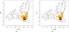 |
Fig. 8 Contour density plot of the Teff – log (g) predictions in the PASTEL catalogue (Soubiran et al. 2010) with our KT (left) and ELODIE (right) predictions for the CoRoT targets observed with the Giraffe spectrograph superimposed as orange dots. |
Excerpt from the full catalog of identifiers, stellar and time series parameters, and variability types for CoRoT targets with Giraffe spectra.
Ideally, an iterative approach could be implemented in which the results obtained from the regression models shown above would be used to improve the reduction stage with parameters optimised for each temperature range. In practice, this would imply a better signal-to-noise ratio. However, for the variability types considered here (see below) this improved ratio would not have a strong impact in the derived classification because variability types that overlap heavily in the parameter space defined by the time series, are characterised by very different temperature ranges (see below).
We measure the robustness of these temperature estimates to inaccuracies in the corrections for the Doppler effect by analysing the change in the model predictions for spectra differing from our corrections by plus/minus one pixel which corresponds to ± 0.2 Å or ± 15 km s-1 at the spectral dispersion of the data. This overestimates the typical errors of cross-correlation estimates of the Doppler shifts, and thus, provides an upper limit to the propagated errors in the derived physical parameters. As a result of the analysis, we find that the 1-σ interval radius for the predictions with a 1 pixel shift with respect to our Doppler corrections is typically 0.02 dex, and 0.24 dex in gravity. Since variability types that overlap in the space of time series parameters are separated by temperature differences far greater than this (see Sect. 4), uncertainties in the radial velocity corrections are not expected to affect the classification in any respect.
3.3. Determination of the gravity
The surface gravity prediction was performed in terms of log (g) using a regression model trained with the synthetic libraries (Kurucz and TLUSTY). In this case, the best model judged by estimating the prediction errors for the ELODIE (independent) dataset did not include sub-models specialised in different temperature or gravity ranges. These more complex models were built and tested, but none showed statistically significant differences in performance (judged again based on the classification errors when applied to ELODIE spectra) with respect to the simpler unique model. Therefore, in the absence of evidence in favour of the more complex models, the simpler model was used in the variability class predictions described in Sect. 4. As in the case of the effective temperature determination, we avoided the inclusion of examples from the two model families (Kurucz and TLUSTY) for the same physical parameters. Again, we used only Kurucz models for effective temperatures below 10 000 K and TLUSTY models above 15 000 K, and therefore, predicted values in the intermediate range are effectively interpolated from the mappings in the boundaries of validity.
The RMSE of this model is 0.3 dex for the test set of synthetic spectra not used for training (33% of the entire synthetic libraries, obtained through random sampling), and 0.6 dex for the independent test set of ELODIE spectra. Figure 7 shows the log (g) predictions as a function of the values tabulated in the ELODIE catalog. The colour code represents the metallicities taken also from the ELODIE catalog. The plot shows a tendency to overestimate the gravity in the low metallicity regime, and to underestimate it for metal-rich stars. We see in degeneracy plots, similar to those shown in Fig. 3, that gravity and metallicity have correlated effects in the spectra, in the same sense as suggested by Fig. 7. Thus, we interpret this systematic trend as a result of this degeneracy, and the decreased spectral information in metal-poor stellar spectra. The presence of anomalous metal abundances in our sample would not affect the classification results described in Sect. 4, but can result in inaccurate estimations of log (g) for these stars.
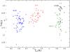 |
Fig. 9 Teff and log (g) values taken from the literature for confirmed δ Sct, β Cep, SPB and γ Dor stars. |
As a final check of the plausibility of the Teff – log (g) predictions we compared their distribution with that of a totally independent dataset not used in any of the training or testing steps taken to construct the regression models. Figure 8a shows the density distribution of values in the PASTEL catalogue with continuous contour lines, together with our KT predictions for the CoRoT targets observed with Giraffe superimposed in orange. Figure 8b shows the same plot using the ELODIE Teff predictions instead. In the computation of the contour lines we have not filtered the PASTEL database in any respect. Thus, we have used all parameter values, even if some correspond to various observations of the same star with different qualities.
The comparison between the PASTEL dataset distribution in parameter space and our predictions for CoRoT targets shows a good overall agreement. CoRoT target selection in the exo-planet fields results in an underabundance of evolved objects with respect to dwarf and sub-giant stars. This is visible as a steep decrease in the number of predictions in the region 2.5 < log (g) < 3 and a complete lack of predictions for lower gravities. The Teff predictions of the ELODIE regression model show less scatter than those of the KT model, and both models yield an overabundance of stars in two regions: red sub-giant stars with log (g) values below 3.1, and Main Sequence stars with temperatures 3.8 < log (Teff) < 4. In both cases, the overbundances follow the contour line shapes and slopes delineated by the PASTEL database, specially in the case of the ELODIE model. There is also a clear underabundance of dwarf stars with temperatures below approximately log (Teff) = 3.7, due to the exoplanet fields limiting magnitude of 16.
Dimensionality reduction techniques based on projection schemes such as those used here have often the drawback that the parameters derived from representations in the reduced space fall outside the convex hull defined by the examples in the training set. This is not the case with the CoRoT spectra analysed in this section, as can be deduced from the comparison of Figs. 2 and 8 (see below). It is not the case either for the ELODIE regression model, although in this case the training set is characterised by a very inhomogeneous coverage of the parameter space and we certainly have predicted parameters in regions with a low density of examples.
Table 2, a complete version of which is available at the CDS2, shows an excerpt of the catalogue obtained as a result of this work. It includes CoRoT identifiers, equatorial coordinates α and δ, variability classes assigned as described in the next Section, the corresponding class probability, the Mahalanobis distance to the center of the class, the first detected frequency, the KT-model and ELODIE-model Teff predictions, and the KT log (g) predictions. The full catalog at CDS also includes the CoRoT run in which the target was observed, the mean V magnitude, the second detected frequency, the amplitudes of the first Fourier terms of the first two detected frequencies, and the p-values (statistical significance) of the frequency detections.
4. Variability classification with temperatures and gravities
Using classification attributes derived from single-bandpass light curves is insufficient to obtain reliable separation of all stellar variability classes. As described in Debosscher et al. (2009), it is impossible to distinguish δ Sct stars from β Cep stars, and γ Dor stars from SPB stars without the use of at least some additional colour information. Given the importance of these pulsating stars for asteroseismological studies, we have extended our supervised classification method to include spectral attributes as well. Since we want to make the classifier as generally applicable as possible, it is important to use classification attributes that are not survey/instrument specific. We therefore chose to use parameters such as Teff and log (g), although they are model dependent, they are not survey dependent, as is the case for certain colour indices derived from observed medium-resolution spectra. Moreover, as shown in the previous section, these parameters can be derived with sufficient accuracy in an automated way, using observed spectra as a starting point.
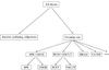 |
Fig. 10 Schematic view of the supervised classification tree. The spectral attributes Teff and log (g) are used in the lowest level, to distinguish δ Sct from β Cep and SPB from γ Dor stars. |
When using supervised classification methods, the classes need to be defined in advance (constituting the training set). To take the parameters Teff and log (g) into account in the classification process, ideally we should have those parameters available for all the objects in the existing training set used to derive the distributions of light curve parameters. This is not possible at this stage, since we do not have estimates available for those fundamental parameters for the majority of the targets in our training set. Luckily, some variability types can be identified reliably using only light curve information, so we actually do not need to extend the training set for all classes. Here, we focused on the separability of four classes of multiperiodic pulsators (δ Sct, β Cep, SPB and γ Dor), for which spectroscopic information is essential to distinguish them. For those classes, we constructed an extended training set, by using Teff and log (g) values taken from confirmed class members in the literature. For the β Cep and the SPB classes, we used the extensive tables compiled by P. De Cat3, for the δ Sct class, we used the catalogue by Rodríguez et al. (2000), and for the γ Dor class we used the lists presented in Cuypers et al. (2009), Aerts et al. (1998), and Handler (1999). The resulting samples are shown in Fig. 9. Clearly, δ Sct stars can be separated from β Cep stars and γ Dor stars from SPB stars in the Teff − log (g) plane. To include these spectral parameters in the classification process, we adapted the existing classification tree by first merging the classes δ Sct with β Cep, and SPB with γ Dor. A new stage was then added to refine the classification within these two subgroups, using the parameters Teff and log (g). Figure 10 represents the classification process in a schematic way. Similar to the methods described in Debosscher et al. (2007) and Blomme et al. (2011), we use a multistage approach, albeit with a simpler tree structure and different classification attributes (our classifier has been designed for application to high quality space-based data). The multistage approach has several advantages: dedicated classifiers can be designed for each split in the tree, each using an optimized set of attributes. Moreover, there is no need to have all classification attributes available for each object in the training set. For example, we only needed Teff and log (g) values for those training classes present in the branches of the tree using these classification attributes.
In the current version of the classifier, we treat Teff and log (g) as statistically independent from the other light curve attributes, since we do not have these parameters available for the training objects used to derive the light curve parameters. Future extensions of the training set should allow for a fully covariant Gaussian Mixture modelling of the distributions of all the classification attributes together.
Number of good candidate variability class members obtained without and with the use of additional spectral classification attributes.
The variability types obtained with the KT and ELODIE Teff predictions coincide in all cases except for three stars. CoRoT 100724564 is a δ Sct type variable with a KT model prediction in the correct temperature range, but the ELODIE model predicts 20 000 K and induces the wrong variability type (β Cep) for the given pulsation frequencies (above 7 cycles/day). On the other hand, the KT model predicts an effective temperature around 10 000 K for CoRoT 110840602 (frequencies above 3 cycles/day) while the ELODIE model predicts a temperature around 20 000 K. The signal-to-noise ratios of the spectrum and the time series are low, but it shows spectral characteristics of B8 stars. Therefore, the classification based on the ELODIE Teff value (β Cep) is to be prefered to the KT-based classification (δ Sct type). A similar situation is found for CoRoT 101486436 which, depending on the spectrum and regression module, maybe classified as δ Sct or β Cep. It is indeed a late B-type star with an ELODIE prediction around 15 500 K, and a KT prediction around 10 000 K. Therefore, the ELODIE Teff prediction is more accurate, and the β Cep class is to be prefered.
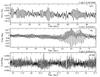 |
Fig. 11 Examples of CoRoT light curves of new candidate hot pulsating stars identified using the spectral classifier. From top to bottom: SPB candidate, Be candidate and β Cep candidate. |
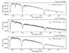 |
Fig. 12 Giraffe spectra in the blue wavelength range (LR2), for the candidate hot pulsating stars shown in Fig. 11, in the same order. |
 |
Fig. 13 Giraffe spectrum in the red wavelength range (LR6) for the Be star CoRoT 102686433, showing strong emission in the Hα line. |
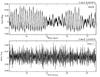 |
Fig. 14 Examples of CoRoT light curves of new candidate cool pulsating stars identified using the spectral classifier: a γ Dor candidate (top) and a δ Sct candidate (bottom). |
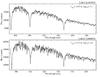 |
Fig. 15 Giraffe spectra in the blue wavelength range (LR2), for the candidate cool pulsating stars shown in Fig. 14, in the same order. Note that these spectra look noisier compared to those of the hot stars, but this is in fact because of the many spectral lines that are present. |
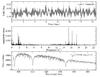 |
Fig. 16 CoRoT light curve, corresponding amplitude spectrum and Giraffe spectrum in the blue wavelength range of a candidate hybrid γ Dor-δ Sct pulsator. |
Table 3 compares the classification results using only light curve (LC) attributes with those obtained using additional spectral attributes. Clearly, the number of candidate SPB and β Cep pulsators drastically decreased by using the spectral attributes, in favour of the δ Sct and γ Dor classes. This is what we expect from the initial mass function: SPB and β Cep stars are more massive and thus rarer objects. We found similar results for the fields observed by the Kepler space mission, as described in Debosscher et al. (2011). In the latter work, we used 2MASS colour indices to distinguish SPB from γ Dor and δ Sct from β Cep after the initial light curve classification. Given their importance for asteroseismological studies and the fact that they are relatively rare, we are especially interested in identifying new members of those variability classes. We selected the best candidates based on the Mahalanobis distance (see Debosscher et al. 2009). The CoRoT light curves of some of the best SPB and β Cep candidates are shown in Fig. 11, their corresponding Giraffe spectra in the blue wavelength range are shown in Fig. 12. One of them actually shows Be-star characteristics in the light curves: sudden amplitude changes and trends. Visual inspection of the Giraffe spectra in the longer wavelength range (LR6) revealed it to be a Be star indeed, as evidenced by the Hydrogen emission (see Fig. 13). It is not surprising that these objects end up in the SPB class, given their similar pulsation characteristics and temperatures. In total, we identified 9 Be stars, 8 of which are classified as SPB, and one as β Cep (those are not included in the numbers of SPB and β Cep candidates in Table 3). They all show clear Hydrogen emission in the Giraffe spectra, and their light curves show amplitude variability in combination with trends. The number of Be stars we find is quite high, compared to the number of other pulsating B-stars (SPB and β Cep). It is expected that about 12−17% of all B stars are Be stars (see e.g. Porter & Rivinius 2003). The fraction we find is very different, but based on a small sample only. The fraction of pulsating B stars amongst all B stars is poorly known, making it hard to judge how significant these differences are at this stage.
Figure 14 shows two examples of new candidate cool pulsators identified using the spectral classifier: a γ Dor candidate and a δ Sct candidate. The γ Dor candidate was previously classified (without spectral attributes) as SPB, while the δ Sct candidate was already classified as such, but could now be classified much more confidently. Figure 15 shows their corresponding Giraffe spectra in the blue wavelength range.
Within our samples of γ Dor and δ Sct pulsators, we could also identify 28 good candidate hybrid pulsators, having pulsation frequencies in both the g-mode and p-mode regimes. These objects are very important for asteroseismic studies, since the presence of both pulsation modes allows us to probe the stellar interior in greater detail. Our current classifier does not have a separate category for these “mixed” pulsators, but we can detect them by inspecting the pulsation frequencies we derived from the CoRoT light curves.
With the current quality of light curves measured from space, the third frequency can provide useful information, especially for multi-periodic targets with mixed types of variability such as hybrid pulsators. We used it here to select hybrids amongst the γ Dor and δ Sct candidates in a manual way, after initial automated classification including only two frequencies. Hybrids have pulsation frequencies in both the p-mode and g-mode regimes, so at least two frequencies are necessary to detect them. Considering more frequencies increases the detection chance, e.g. in the case where the two most dominant modes are g-modes, and the third one a p-mode, or vice versa. The first discordant frequency (i.e., the first frequency of a pulsating mode, p- or g-, different from the first one) can appear in any position from the second one onward (up to hundreds of frequencies). Thus, the number of frequencies analysed is somehow arbitrary, and as a consequence, the distinctions between δ Sct/hybrid and γ Dor/hybrid may change. We plan to extend our classifiers to detect hybrids in an automated way in the future.
Recent results from the even longer time series of Kepler data (Grigahcène et al. 2010) suggest that most γ Dor and δ Sct pulsators might in fact be hybrids. Extending the sample for such stars is essential to investigate the link between both types of pulsators (both observational and theoretical), given their overlap in pulsational instability domains. Most of the hybrids (23) in our sample have dominant pulsation frequencies in the p-mode regime (roughly above 5 d-1), similar to what Grigahcène et al. (2010) found, although the ratio is more extreme in our case.
Figure 16 shows the CoRoT light curve (detrended with a third-order polynomial), the corresponding amplitude spectrum and the Giraffe spectrum in the blue wavelength range (LR2) of one of the candidate hybrid pulsators. Note the occurrence of clear groups of pulsation frequencies around 2 d-1 (g-mode regime) and around 16 d-1 (p-mode regime) in the amplitude spectrum. The Giraffe spectrum is compatible with an early F spectral type, and the predicted temperature for this star is about 7300 K, typical for both γ Dor and δ Sct pulsators.
Similar to hybrid γ Dor-δ Sct pulsations, also hybrid SPB-β Cep pulsations are known, see e.g. Degroote et al. (2012) for an example in the CoRoT seismology data. We also checked our sample of candidate SPB and β Cep pulsators for the occurrence of both g and p-mode pulsations, but we found no convincing candidate hybrids.
Although we focus on the separability of four classes of pulsators using spectral attributes, Table 3 also lists the results for the other variability types we identified in the CoRoT sample. The classification results for these classes did not change after the inclusion of the spectral attributes Teff and log (g), since they only affect the relative class probabilities for the combinations of classes SPB/γ Dor and δ Sct/β Cep. No spectral information is needed for a reliable identification of these variability types, since the light curves are very characteristic. In some cases, such as for eclipsing/ellipsoidal binaries, spectral attributes will decrease the quality of the classification. For RR-Lyrae stars, even though they are located within a well defined region in the Teff − log (g) plane, light curve attributes derived from high quality space-based data always provide more reliable classification parameters, such as the phase differences between harmonics or the frequency ratio in the case of double-mode RR Lyrae (RRd) stars.
Compared to our CoRoT light curve classification results presented in Debosscher et al. (2009), our classifier can now also identify light curves with signs of rotational modulation (stellar spots). In Debosscher et al. (2011), we identified a large sample of these stars in the Kepler data and studied their location in 2MASS colour space. Similarly, we can evaluate the CoRoT sample of these stars in an independent way by using the derived Teff − log (g) values. Figure 17 plots the CoRoT sample of the best rotational modulation candidates (again using thresholds on the class probability and the Mahalanobis distance) in the Teff − log (g) plane. The CoRoT δ Sct sample is shown for comparison. The bulk of the candidates occupies a well defined region, corresponding to cool main sequence stars, similar to the Kepler results. This is indeed where we expect to find most of these stars. Even though Teff and log (g) are not used to identify those stars by the classifier, they are clearly separated from the pulsating stars, showing that the light curves contain sufficient information to identify them. Remarkably, we also find a few candidates at much higher temperatures. Figure 18 shows two examples of CoRoT light curves in the rotational modulation sample. The upper light curve corresponds to an object present near the center of the main group of cool stars, while the lower light curve corresponds to one of the few much hotter stars. Visual inspection of several other light curves revealed that many of the stars present in the main group show typical signs of rotational modulation, while the few hotter targets seem to have more periodic light curves, stable over a longer period of time. These hotter stars could be chemically peculiar stars, where the rotational variability in the light curve is caused by magnetic fields. Note that the CoRoT seismology programme revealed several more and even hotter cases of OB stars with rotational modulation, often in combination with stellar pulsation (see Degroote et al. 2011; Pápics et al. 2011).
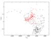 |
Fig. 17 Rotational modulation candidates in the Teff − log (g) plane (black circles), with the δ Sct sample shown for comparison (red squares). |
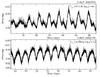 |
Fig. 18 Two examples of CoRoT light curves of rotational modulation candidates, from very different regions in the Teff − log (g) plane. |
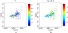 |
Fig. 19 δ Sct candidates in the Teff − log (g) plane. The frequency (measured in cycles per day; left) and the base-10 logarithm of the amplitude of the first term in its Fourier decomposition (right) are represented using the colour codes shown at the right of each plot, and circles of radii proportional to the value. |
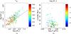 |
Fig. 20 Distribution of amplitudes in the category of δ Sct candidates. The left-hand plot shows the distribution of the amplitudes of the first two terms in the Fourier decomposition of the first frequency in logarithmic scale. The colour code and circles radii represent the effective temperature. The right-hand plot shows the distribution of amplitudes of the first Fourier component of the first frequency as a function of the position in the log 10(Teff)–ν1 plane. Black circles represent hybrid pulsators. |
5. Discussion
In what follows, we review the distribution of CoRoT targets in parameter space for the two variability types with a number of candidate stars that justifies a search for correlations, namely δ Sct and γ Dor stars. All figures in this Section are plot using the ELODIE Teff predictions. The general conclusions drawn from the plots hold both for KT and ELODIE Teff predictions, but ELODIE values show less scatter and the various samples are more localised in the Teff – log (g) plane.
Figure 19 shows the distribution of δ Sct candidates in the Teff – log (g) plane. The colour code reflects the value of the first frequency (in cycles per day, Fig. 19a) and the base-10 logarithm of the amplitude of the first term in its Fourier decomposition A11 (Fig. 19b). Black circles represent candidates of the category of hybrid pulsators discussed in the previous section. The two figures show a separation between less evolved stars, closer to the Main Sequence and characterised by slightly higher frequencies and lower amplitudes, and giant stars with lower frequencies and higher amplitudes.
We also find a separation between hotter and cooler δ Sct candidates in the space of harmonic amplitudes. Figure 20a shows the scatter plot of candidates in the log 10(A11)–log 10(A12) plane. Here, A12 refers to the second term in the Fourier decomposition of the first frequency component of the time series. The black line has a slope equal to one, and shows a tendency for the larger amplitude time series to deviate more from the sinusoidal shape (larger A12/A11 ratios). Again, black circles represent hybrid pulsators.
The Teff-ν1 plot (Fig. 20b) is qualitatively similar to previous studies (see e.g. Balona & Dziembowski 2011), except for the presence of high frequency (ν1 > 40 cycles/day) δ Sct stars down to log (Teff) = 3.85.
The analysis of the γ Dor candidates does not show clear indications of correlations. Figures 21a and b show the Teff – log (g) scatter plot, with frequencies (left) and amplitudes (right) reflected in the colour code and radii of the circles. Black circles represent hybrid pulsators as in the previous figures.
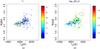 |
Fig. 21 γ Dor candidates in the Teff − log (g) plane. The frequency (left) and the amplitude of the first term in its Fourier decomposition (right) are represented using the colour codes shown at the right of each plot, and circles of radii proportional to the value. Frequencies are measured in cycles per day. Black circles represent hybrid pulsators. |
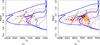 |
Fig. 22 δ Sct (red), γ Dor (orange), and hybrid (black) candidate stars in the Teff – log (g) plane. The left-hand diagram shows the distribution of Kepler candidates according to Uytterhoeven et al. (2011). We show only values derived from spectroscopy and with uncertainties in the effective temperatures below 100 K (filled circles) or below 240 K (empty symbols). The right-hand plot corresponds to our determination of the parameters for CoRoT candidates. Black continuous lines represent evolutionary tracks for stars with M/M⊙ = 2.5, 2.0, 1.5 and 1.0 and Z = 0.019 from Marigo et al. (2008). The thick straight lines represent the instability regions for δ Sct-type pulsation (red) from Rodríguez & Breger (2001) and for γ Dor-type pulsation (orange) from Handler & Shobbrook (2002). The blue thick lines represent isochrones from the same set of evolutionary tracks for ages log (t /yrs) = 8.5, 9.0, and 9.5 dex. |
In Fig. 22 we compare the distribution of both δ Sct and γ Dor stars in the CoRoT sample (right) with the Kepler sample (left) by Uytterhoeven et al. (2011). Whilst the physical parameters of the CoRoT sample stars were derived through a homogeneous procedure applied to ground-based spectra, those of the Kepler sample stars come from various sources, including values taken from the literature, fits to multi-colour Sloan or Strömgren photometry, and ground-based spectra of different spectral resolutions (see Uytterhoeven et al. (2011) for a more detailed description of the procedures). Figure 22 only shows Kepler targets with spectroscopic observations, and uncertainties in the temperature determinations below 240 K (empty symbols) or below 100 K (filled circles). None of them is associated to an eclipsing binary system. Selected evolutionary tracks (M/M⊙ = 2.5, 2.0, 1.5, and 1.0) and the observed instability regions (red for δ Sct and orange for γ Dor stars) are superimposed in the scatter plots. The thick blue lines represent isochrones for ages log (t /yrs) = 8.5, 9.0, and 9.5.
The comparison of the CoRoT and Kepler samples shows that the two agree in a picture where the previously accepted instability regions fail to account for the physical parameters of many targets. In particular, both samples of γ Dor candidates are characterised by lower gravities than predicted by the pulsation models. The effective temperatures of these stars mostly concentrate near and to the right of the red edge of the strip, although both samples also contain targets bluer (hotter) than the blue edge of the γ Dor strip. The samples of δ Sct hybrid pulsators also spread over a much wider region than predicted by the instability strips, both in mass and evolutionary state.
If we compare our log (g) predictions for the ELODIE dataset, with the values tabulated in the catalog (Fig. 7), we find that our regression models tend to predict values that are lower than the ELODIE catalog values by 0.05 dex (median value) in the range 3.5 < log (g) < 4.0, and 0.24 dex (also median value) between 4.0 and 4.5 dex. When this latter value is calculated from a sample of ELODIE stars restricted to the range 6500 K <Teff< 7500 K, it increases to 0.36 dex. Therefore, it cannot be discarded that the difference in average gravity between Kepler and CoRoT γ Dor candidates in the Teff – log (g) plane is mainly due to a bias induced by the fact that the two predictions (the ELODIE catalog and our predictions) are due to intrinsically different models. One is based on a compilation of heterogeneous bibliographic references and the other is based (in the realm of the γ Dor stars) on the Kurucz library. Therefore, it is not surprising if the two models disagree to some extent in their mapping between spectra and parameters.
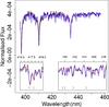 |
Fig. 23 Median spectrum of the CoRoT targets with effective temperatures between 6800 and 7200 K and gravities between 3.5 and 4.0 dex (black). We also show for comparison the Kurucz spectra for Teff = 7000 K and log (g) values equal to 3.0 (red), 4.0 (violet), and 5.0 dex (blue). The left inset box contains a close-up of the spectral range between 416 and 419 nm, around the luminosity-dependent double blend of Feii and Tiii lines at 417.2/417.8 nm. The right-hand inset shows a similar close-up between 441 and 448 nm, with similar blends at 439.5−440 nm, 441.7 nm, and 444.4 nm, and showing no luminosity dependence in the 3.0 ≤ log (g) ≤ 5.0 range. |
The shift towards lower gravities in the γ Dor CoRoT sample could also be explained as the result of the bias discussed in previous sections, in the sense that higher metal abundances can induce lower estimated surface gravities. However, we find it unlikely that these stars are all metal-rich stars compared to the Sun, especially because the Kepler parameters, estimated in an independent way, also show this displacement from the theoretical instability strip towards lower gravities. We have analysed the distribution of surface gravities as a function of apparent V magnitude in the samples of δ Sct and γ Dor stars separately for the center and anti-center fields, and found no significant trend, nor differences between the mean or median values per field. It cannot be discarded that stars in the CoRoT center field are more metal-rich than in the opposite direction, but if this is the case, it does not translate into lower gravities in our determinations. Therefore, we believe that we can discard a metallicity difference as the origin of the low gravities (as compared to the instability strip) in the γ Dor sample.
In order to confirm the plausibility of this shift in the typical surface gravities of γ Dor stars, we have analysed luminosity sensitive spectral lines in the LR2 wavelength range. Figure 23 shows the Kurucz spectra for Teff = 7000 K, and log (g) = 3.0 (red), 4.0 (violet), and 5.0 (blue). We also show the median spectrum of CoRoT targets in the γ Dor category with effective temperatures between 6800 and 7200 K, and gravities between 3.5 and 4.0 dex (black). The inset shows the region between 416 and 419 nm in greater detail. This wavelength range includes the luminosity-dependent double blend of Feii and Tiii at 417.2/417.8 nm. All four spectra have been continuum subtracted and normalised to yield an area under the spectrum equal to one. The plot shows that the best agreement between a Kurucz spectrum and the median spectrum of CoRoT targets is achieved by the Kurucz model with log (g) = 3.0, thus confirming that the log (g) values predicted by our regression model reflect the mapping between spectra and gravities that is inherent to the Kurucz library of spectra.
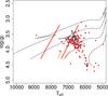 |
Fig. 24 Positions in the Teff – log (g) plane of the CoRoT γ Dor candidates in the center (grey) and anticenter (red) fields. The instability strips and evolutionary tracks are the same as those represented in Fig. 22. |
We interpret this as an indication that, at least in the stellar populations probed by the CoRoT and Kepler fields (i.e. near the Galactic disk), and in the light of the Kurucz library of models, the observed instability region for γ Dor-type pulsation extends to lower gravities, as in the case of the δ Sct instability region.
Figure 24 shows the distribution of γ Dor candidates separately for the center (grey) and anti-center (red) fields of the so-called CoRoT eyes (the regions of the sky accessible to CoRoT, in the intersections between the Galactic and equatorial planes; see Boisnard & Auvergne 2006). Overall, the anticenter direction provides 2.5 times as many γ Dor candidates as the center fields. In the region defined by Teff< 6500 K and log (g) > 4, there are 4.5 times as many. This may indicate that the anticenter direction is conveying an additional population of stars in the γ Dor category characterised by lower temperatures and higher gravities.
In general, we find strong indications that the instability regions for both δ Sct and γ Dor variability extend far beyond their previously observed edges. This extension however does not imply changes in the energy-efficiency diagram proposed in Uytterhoeven et al. (2011), that shows the same distribution as presented therein for Kepler targets (see Fig. 25). Energy there is defined as (Amaxζ)2, where Amax and ζ are the maximum amplitude and associated frequency observed in a pulsation mode of a given time series, and efficiency is defined as (Teff3log (g))− 2/3.
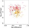 |
Fig. 25 Energy and efficiency of δ Sct (red) and γ Dor (orange) candidate stars according to the definitions by Uytterhoeven et al. (2011). Black circles represent hybrid stars. |
6. Summary
In this work we have presented an improved variability classification of a subset of CoRoT target stars in the exo-planet fields, consisting of 6832 variable stars observed with the Giraffe multi-object spectrograph. For this set of stars and using regression techniques based on Support Vector Machines, we derive Teff and log (g) estimates that allow us to refine and improve the variability class assignments provided in Debosscher et al. (2009). This is accomplished with a new variability classifier that makes use of the new information available (Teff and log (g)) to separate variability types that heavily overlap in the space of parameters derived only from single-band photometric time series (namely, the δ Sct–β Cep types, and the γ Dor-SPB types).
We estimate the Root Mean Squared Errors in the Teff estimates to be 400 K for the temperature range Teff< 10 000 K, and 4000 K for temperatures above 10 000 K. This accuracy is sufficient to separate the variability types mentioned in the previous paragraph. We provide this improved variability classification together with the stellar parameters in a catalog available from the CDS. It contains amongst others 330 γ Dor, 343 δ Sct, 8 SPB and 6 β Cep candidates.
The analysis of our CoRoT samples of γ Dor and δ Sct stars yields the following conclusions:
-
1.
We find hints of an evolution in the pulsational properties ofδ Sct stars across the HR diagram, in the sense that more evolved stars show lower frequencies and higher amplitudes than stars closer to the Main Sequence.
-
2.
The distributions of the CoRoT candidate δ Sct and γ Dor stars spread over a much wider area in both Teff and log (g) than previously observed.
-
3.
The largest concentration of γ Dor candidates in the Teff − log (g) planes occurs at surface gravities between 3.5 and 4.0 dex, in an extension of the previously observed instability region for this variability type.
-
4.
The number of candidate δ Sct and γ Dor pulsators we identified is significantly higher (a factor of two to three) in the galactic anticenter direction of the CoRoT observations compared to the center direction, even though we have more spectra available for the center direction.
This work concentrated on CoRoT stars observed in the LR2 setup of the Giraffe spectrograph. There is still a large number of stars (1230) that have only LR6 spectra available and, although not as informative as the LR2 wavelength range for the Teff estimation, can still provide sufficient approximations
for the variability classification. This will be the objective of a forthcoming paper.
Centre de Données astronomiques de Strasbourg, http://cdsweb.u-strasbg.fr/
Available at http://www.ster.kuleuven.be/~peter/Bstars/
Acknowledgments
This research was supported by the Spanish Ministry of Economy and Competitiveness through grants AyA2008-02156 and AyA2011-24052. The research leading to these results has received funding from the European Research Council under the European Community’s Seventh Framework Programme (FP7/2007–2013)/ERC grant agreement n°227224 (PROSPERITY), from the Research Council of K.U.Leuven (GOA/2008/04), and from the Belgian federal science policy office (C90309: CoRoT Data Exploitation).
References
- Aerts, C., Eyer, L., & Kestens, E. 1998, A&A, 337, 790 [NASA ADS] [Google Scholar]
- Allende Prieto, C., Rebolo, R., García López, R. J., et al. 2000, AJ, 120, 1516 [NASA ADS] [CrossRef] [Google Scholar]
- Auvergne, M., Bodin, P., Boisnard, L., et al. 2009, A&A, 506, 411 [NASA ADS] [CrossRef] [EDP Sciences] [Google Scholar]
- Bailer-Jones, C. A. L. 2000, A&A, 357, 197 [NASA ADS] [Google Scholar]
- Bailer-Jones, C. A. L. 2010, MNRAS, 403, 96 [NASA ADS] [CrossRef] [Google Scholar]
- Balona, L. A., & Dziembowski, W. A. 2011, MNRAS, 417, 591 [NASA ADS] [CrossRef] [Google Scholar]
- Bertone, E., Buzzoni, A., Chávez, M., & Rodríguez-Merino, L. H. 2008, A&A, 485, 823 [NASA ADS] [CrossRef] [EDP Sciences] [Google Scholar]
- Bijaoui, A., Recio-Blanco, A., de Laverny, P., & Ordenovic, C. 2010, in ADA 6 – Sixth Conference on Astronomical Data Analysis [Google Scholar]
- Bishop, C. M. 1995, Neural Networks for Pattern Recognition (New York, NY, USA: Oxford University Press, Inc.) [Google Scholar]
- Blomme, J., Sarro, L. M., O’Donovan, F. T., et al. 2011, MNRAS, 418, 96 [NASA ADS] [CrossRef] [Google Scholar]
- Boisnard, L., & Auvergne, M. 2006, in ESA SP 1306, eds. M. Fridlund, A. Baglin, J. Lochard, & L. Conroy, 19 [Google Scholar]
- Cao, L. J., Chua, K. S., Chong, W. K., Lee, H. P., & Gu, Q. M. 2003, Neurocomputing, 55, 321 [CrossRef] [Google Scholar]
- Coifman, R., & Lafon, S. 2006, Appl. Comput. Harmonic Analys., 21, 5 [Google Scholar]
- Cortes, C., & Vapnik, V. 1995, Machine Learning, 20, 273 [Google Scholar]
- Cover, T. M., & Hart, P. E. 1967, IEEE Transactions on Information Theory, 13, 21 [Google Scholar]
- Cuypers, J., Aerts, C., De Cat, P., et al. 2009, A&A, 499, 967 [NASA ADS] [CrossRef] [EDP Sciences] [Google Scholar]
- Daszykowski, M. 2007, J. Chemometrics, 21, 270 [CrossRef] [Google Scholar]
- Debosscher, J., Sarro, L. M., Aerts, C., et al. 2007, A&A, 475, 1159 [NASA ADS] [CrossRef] [EDP Sciences] [Google Scholar]
- Debosscher, J., Sarro, L. M., López, M., et al. 2009, A&A, 506, 519 [NASA ADS] [CrossRef] [EDP Sciences] [Google Scholar]
- Debosscher, J., Blomme, J., Aerts, C., & De Ridder, J. 2011, A&A, 529, A89 [NASA ADS] [CrossRef] [EDP Sciences] [Google Scholar]
- Degroote, P., Acke, B., Samadi, R., et al. 2011, A&A, 536, A82 [NASA ADS] [CrossRef] [EDP Sciences] [Google Scholar]
- Degroote, P., Aerts, C., Michel, E., et al. 2012, A&A, 542, A88 [NASA ADS] [CrossRef] [EDP Sciences] [Google Scholar]
- Eisenstein, D. J., Weinberg, D. H., Agol, E., et al. 2011, AJ, 142, 72 [Google Scholar]
- Fodor, I. K., & Kamath, C. 2002, Computat. Statist. Data Analys., 41, 91 [CrossRef] [Google Scholar]
- Gilmore, G., Randich, S., Asplund, M., et al. 2012, The Messenger, 147, 25 [NASA ADS] [Google Scholar]
- Grigahcène, A., Antoci, V., Balona, L., et al. 2010, ApJ, 713, L192 [NASA ADS] [CrossRef] [Google Scholar]
- Handler, G. 1999, MNRAS, 309, L19 [NASA ADS] [CrossRef] [Google Scholar]
- Handler, G., & Shobbrook, R. R. 2002, MNRAS, 333, 251 [NASA ADS] [CrossRef] [Google Scholar]
- Hubeny, I., & Lanz, T. 1995, ApJ, 439, 875 [Google Scholar]
- Japkowicz, N., & Stephen, S. 2002, Intell. Data Anal., 6, 429 [Google Scholar]
- Jofré, P., Panter, B., Hansen, C. J., & Weiss, A. 2010, A&A, 517, A57 [NASA ADS] [CrossRef] [EDP Sciences] [Google Scholar]
- Kordopatis, G., Recio-Blanco, A., de Laverny, P., et al. 2011, A&A, 535, A106 [NASA ADS] [CrossRef] [EDP Sciences] [Google Scholar]
- Lee, Y. S., Beers, T. C., Sivarani, T., et al. 2008, AJ, 136, 2022 [NASA ADS] [CrossRef] [Google Scholar]
- Marigo, P., Girardi, L., Bressan, A., et al. 2008, A&A, 482, 883 [NASA ADS] [CrossRef] [EDP Sciences] [Google Scholar]
- Marshall, R. 2002, Statistics in Medicine, 21, 1966 [CrossRef] [Google Scholar]
- Pápics, P. I., Briquet, M., Auvergne, M., et al. 2011, A&A, 528, A123 [NASA ADS] [CrossRef] [EDP Sciences] [Google Scholar]
- Porter, J. M., & Rivinius, T. 2003, PASP, 115, 1153 [NASA ADS] [CrossRef] [Google Scholar]
- Prugniel, P., & Soubiran, C. 2001, A&A, 369, 1048 [NASA ADS] [CrossRef] [EDP Sciences] [Google Scholar]
- Prugniel, P., & Soubiran, C. 2004 [arXiv:astro-ph/0409214] [Google Scholar]
- Recio-Blanco, A., Bijaoui, A., & de Laverny, P. 2006, MNRAS, 370, 141 [NASA ADS] [CrossRef] [Google Scholar]
- Rodríguez, E., & Breger, M. 2001, A&A, 366, 178 [NASA ADS] [CrossRef] [EDP Sciences] [Google Scholar]
- Rodríguez, E., López-González, M. J., & López de Coca, P. 2000, A&AS, 144, 469 [NASA ADS] [CrossRef] [EDP Sciences] [Google Scholar]
- Rosipal, R., Be, P. P., Trejo, L. J., et al. 2001, J. Machine Learning Res., 2, 97 [Google Scholar]
- Siebert, A., Williams, M. E. K., Siviero, A., et al. 2011, AJ, 141, 187 [NASA ADS] [CrossRef] [Google Scholar]
- Soubiran, C., Katz, D., & Cayrel, R. 1998, A&AS, 133, 221 [NASA ADS] [CrossRef] [EDP Sciences] [Google Scholar]
- Soubiran, C., Le Campion, J.-F., Cayrel de Strobel, G., & Caillo, A. 2010, A&A, 515, A111 [NASA ADS] [CrossRef] [EDP Sciences] [Google Scholar]
- Suzuki, T., & Sugillama, M. 2011, Neural Computation, 23, 284 [CrossRef] [Google Scholar]
- Uytterhoeven, K., Moya, A., Grigahcène, A., et al. 2011, A&A, 534, A125 [NASA ADS] [CrossRef] [EDP Sciences] [Google Scholar]
- Vapnik, V. N. 1995, The nature of statistical learning theory (New York: NY, USA: Springer-Verlag New York, Inc.) [Google Scholar]
All Tables
Global validation errors (mean absolute and root mean square error) for the ELODIE dataset obtained by predicting the values of Teff and log (g) using only the LR2 range, only the LR6 range, and the combination of the LR2 and LR6 wavelength ranges.
Excerpt from the full catalog of identifiers, stellar and time series parameters, and variability types for CoRoT targets with Giraffe spectra.
Number of good candidate variability class members obtained without and with the use of additional spectral classification attributes.
All Figures
|
Fig. 1 Giraffe spectra of the first two CoRoT targets in the catalog (top). In the middle row, we show the same spectra after continuum subtraction (Fcs(λ)), and the lower row shows the spectra after rescaling (subtraction of the minimum flux and normalisation to unit area; Fscl(λ)). |
| In the text | |
|
Fig. 2 Coverage in parameter space of the training sets used to construct the regression models. Crosses correspond to the Kurucz models and circles to the TLUSTY grid of models. |
| In the text | |
|
Fig. 3 Differences between four selected ELODIE spectra (indexed by the stellar parameters shown in each panel) and the ELODIE spectral collection. The panels show an approximation to the expected degeneracies in the mapping between spectra and physical parameters. The colour code represents the area of the (absolute value of the) difference between two pairs of spectra, where each spectrum has been normalised to area 1, as described in the text. |
| In the text | |
|
Fig. 4 Comparison of the effective temperatures assigned in the ELODIE spectral compilation and those predicted for the ELODIE dataset with Teff< 10 000 K by the non linear SVM model trained with Kurucz spectra with Teff< 10 000 K. The colour code reflects the log (g) value assigned in the ELODIE catalog. |
| In the text | |
|
Fig. 5 Comparison of the effective temperatures assigned in the ELODIE spectral compilation and those predicted for the ELODIE dataset with Teff> 15 000 K by the non-linear SVM model trained with TLUSTY models. The colour code reflects the log (g) value assigned in the ELODIE catalog. |
| In the text | |
|
Fig. 6 Comparison of the Teff predictions by the ELODIE model (x axis) and the KT model (y axis). The median values in bins 0.1 dex wide defined in the x axis are shown in orange, and the median absolute deviations (MAD) are also shown as error bars. |
| In the text | |
|
Fig. 7 Prediction accuracy of the regression model for gravity when applied to the ELODIE dataset. The y-axis represents the predictions from the regression model and the x-axis represents the log (g) values tabulated in the ELODIE catalog. The colour code represents the [Fe/H] values taken from the same catalog. |
| In the text | |
|
Fig. 8 Contour density plot of the Teff – log (g) predictions in the PASTEL catalogue (Soubiran et al. 2010) with our KT (left) and ELODIE (right) predictions for the CoRoT targets observed with the Giraffe spectrograph superimposed as orange dots. |
| In the text | |
|
Fig. 9 Teff and log (g) values taken from the literature for confirmed δ Sct, β Cep, SPB and γ Dor stars. |
| In the text | |
|
Fig. 10 Schematic view of the supervised classification tree. The spectral attributes Teff and log (g) are used in the lowest level, to distinguish δ Sct from β Cep and SPB from γ Dor stars. |
| In the text | |
|
Fig. 11 Examples of CoRoT light curves of new candidate hot pulsating stars identified using the spectral classifier. From top to bottom: SPB candidate, Be candidate and β Cep candidate. |
| In the text | |
|
Fig. 12 Giraffe spectra in the blue wavelength range (LR2), for the candidate hot pulsating stars shown in Fig. 11, in the same order. |
| In the text | |
|
Fig. 13 Giraffe spectrum in the red wavelength range (LR6) for the Be star CoRoT 102686433, showing strong emission in the Hα line. |
| In the text | |
|
Fig. 14 Examples of CoRoT light curves of new candidate cool pulsating stars identified using the spectral classifier: a γ Dor candidate (top) and a δ Sct candidate (bottom). |
| In the text | |
|
Fig. 15 Giraffe spectra in the blue wavelength range (LR2), for the candidate cool pulsating stars shown in Fig. 14, in the same order. Note that these spectra look noisier compared to those of the hot stars, but this is in fact because of the many spectral lines that are present. |
| In the text | |
|
Fig. 16 CoRoT light curve, corresponding amplitude spectrum and Giraffe spectrum in the blue wavelength range of a candidate hybrid γ Dor-δ Sct pulsator. |
| In the text | |
|
Fig. 17 Rotational modulation candidates in the Teff − log (g) plane (black circles), with the δ Sct sample shown for comparison (red squares). |
| In the text | |
|
Fig. 18 Two examples of CoRoT light curves of rotational modulation candidates, from very different regions in the Teff − log (g) plane. |
| In the text | |
|
Fig. 19 δ Sct candidates in the Teff − log (g) plane. The frequency (measured in cycles per day; left) and the base-10 logarithm of the amplitude of the first term in its Fourier decomposition (right) are represented using the colour codes shown at the right of each plot, and circles of radii proportional to the value. |
| In the text | |
|
Fig. 20 Distribution of amplitudes in the category of δ Sct candidates. The left-hand plot shows the distribution of the amplitudes of the first two terms in the Fourier decomposition of the first frequency in logarithmic scale. The colour code and circles radii represent the effective temperature. The right-hand plot shows the distribution of amplitudes of the first Fourier component of the first frequency as a function of the position in the log 10(Teff)–ν1 plane. Black circles represent hybrid pulsators. |
| In the text | |
|
Fig. 21 γ Dor candidates in the Teff − log (g) plane. The frequency (left) and the amplitude of the first term in its Fourier decomposition (right) are represented using the colour codes shown at the right of each plot, and circles of radii proportional to the value. Frequencies are measured in cycles per day. Black circles represent hybrid pulsators. |
| In the text | |
|
Fig. 22 δ Sct (red), γ Dor (orange), and hybrid (black) candidate stars in the Teff – log (g) plane. The left-hand diagram shows the distribution of Kepler candidates according to Uytterhoeven et al. (2011). We show only values derived from spectroscopy and with uncertainties in the effective temperatures below 100 K (filled circles) or below 240 K (empty symbols). The right-hand plot corresponds to our determination of the parameters for CoRoT candidates. Black continuous lines represent evolutionary tracks for stars with M/M⊙ = 2.5, 2.0, 1.5 and 1.0 and Z = 0.019 from Marigo et al. (2008). The thick straight lines represent the instability regions for δ Sct-type pulsation (red) from Rodríguez & Breger (2001) and for γ Dor-type pulsation (orange) from Handler & Shobbrook (2002). The blue thick lines represent isochrones from the same set of evolutionary tracks for ages log (t /yrs) = 8.5, 9.0, and 9.5 dex. |
| In the text | |
|
Fig. 23 Median spectrum of the CoRoT targets with effective temperatures between 6800 and 7200 K and gravities between 3.5 and 4.0 dex (black). We also show for comparison the Kurucz spectra for Teff = 7000 K and log (g) values equal to 3.0 (red), 4.0 (violet), and 5.0 dex (blue). The left inset box contains a close-up of the spectral range between 416 and 419 nm, around the luminosity-dependent double blend of Feii and Tiii lines at 417.2/417.8 nm. The right-hand inset shows a similar close-up between 441 and 448 nm, with similar blends at 439.5−440 nm, 441.7 nm, and 444.4 nm, and showing no luminosity dependence in the 3.0 ≤ log (g) ≤ 5.0 range. |
| In the text | |
|
Fig. 24 Positions in the Teff – log (g) plane of the CoRoT γ Dor candidates in the center (grey) and anticenter (red) fields. The instability strips and evolutionary tracks are the same as those represented in Fig. 22. |
| In the text | |
|
Fig. 25 Energy and efficiency of δ Sct (red) and γ Dor (orange) candidate stars according to the definitions by Uytterhoeven et al. (2011). Black circles represent hybrid stars. |
| In the text | |
Current usage metrics show cumulative count of Article Views (full-text article views including HTML views, PDF and ePub downloads, according to the available data) and Abstracts Views on Vision4Press platform.
Data correspond to usage on the plateform after 2015. The current usage metrics is available 48-96 hours after online publication and is updated daily on week days.
Initial download of the metrics may take a while.