| Issue |
A&A
Volume 550, February 2013
|
|
|---|---|---|
| Article Number | A56 | |
| Number of page(s) | 26 | |
| Section | Interstellar and circumstellar matter | |
| DOI | https://doi.org/10.1051/0004-6361/201220130 | |
| Published online | 24 January 2013 | |
Carbon fractionation in photo-dissociation regions⋆
I. Physikalisches Institut, Universität zu Köln, Zülpicher Str. 77, 50937 Köln, Germany
e-mail: roellig@ph1.uni-koeln.de
Received: 30 July 2012
Accepted: 14 November 2012
We upgraded the chemical network from the UMIST Database for Astrochemistry 2006 to include isotopes such as 13C and 18O. This includes all corresponding isotopologues, their chemical reactions and the properly scaled reaction rate coefficients. We study the fractionation behavior of astrochemically relevant species over a wide range of model parameters, relevant for modelling of photo-dissociation regions (PDRs). We separately analyze the fractionation of the local abundances, fractionation of the total column densities, and fractionation visible in the emission line ratios. We find that strong C+ fractionation is possible in cool C+ gas. Optical thickness as well as excitation effects produce intensity ratios between 40 and 400. The fractionation of CO in PDRs is significantly different from the diffuse interstellar medium. PDR model results never show a fractionation ratio of the CO column density larger than the elemental ratio. Isotope-selective photo-dissociation is always dominated by the isotope-selective chemistry in dense PDR gas. The fractionation of C, CH, CH+ and HCO+ is studied in detail, showing that the fractionation of C, CH and CH+ is dominated by the fractionation of their parental species. The light hydrides chemically derive from C+, and, consequently, their fractionation state is coupled to that of C+. The fractionation of C is a mixed case depending on whether formation from CO or HCO+ dominates. Ratios of the emission lines of [C ii], [C i], 13CO, and H13CO+ provide individual diagnostics to the fractionation status of C+, C, and CO.
Key words: astrochemistry / ISM: abundances / ISM: structure / ISM: clouds / photon-dominated region (PDR)
Appendices are available in electronic form at http://www.aanda.org
© ESO, 2013
1. Introduction
Astronomical observations of molecules and their respective isotopologues reveal, that abundance ratios of the main species to their respective isotopologues may differ significantly from e.g. solar system isotope ratios. While isotopic fractionation in the interstellar medium is widely discussed in the framework of deuterium chemistry, its relevance for the 12C/13C ratio in various species usually gains much less attention. In this paper we investigate chemical fractionation in the context of models of photo-dissociation regions (PDR) with the focus on effects that result from introducing 13C into the applied chemical network.
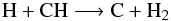
The most important fractionation reaction is
 (C 1)(see Woods & Willacy 2009, and references therein). At high temperature back and forth reaction are equally probable and no apparent deviation from the elemental isotope ratio takes place. The lower the temperature gets, the less probable the back reaction becomes, resulting in a one-way channel shifting 13C into 13CO and decreasing the abundance ratio of 12CO/13CO. At the same time the abundance ratio of 12C+/13C+ is shifted oppositely. Langer et al. (1984) performed numerical calculations of a time-dependant chemical network for a variety of physical parameter and given kinetic temperatures concluding that chemical fractionation of carbon bearing species is of increasing significance the lower the temperate is, confirming the relevance of zero-point energy differences of a few ten K at low temperatures. In dark cloud models, where radiation is usually neglected, the kinetic temperature is the major parameter in opening and closing reaction channels. For a given density, the chemical network only depends on the temperature and the cosmic ray ionization rate ζCR (and history in case of time-dependant calculations).
Carbon fractionation in molecular and diffuse clouds has been discussed systematically by Keene et al. (1998) and Liszt (2007). Following Wakelam & Herbst (2008) we assume a standard elemental abundance of 13C/12C of 67 in the solar neighbourhood. Observing 13[C i] and 13C18O in the Orion Bar Keene et al. (1998) found little evidence for chemical fractionation. Their observations showed a slight enhancement of C18O/13C18O = 75 and no enhancement of [13Ci]/[Ci] relative to the standard elemental abundance while the chemical models predicted the opposite. The systematic study of the C18O/13C18O by Langer & Penzias (1990, 1993) showed a systematic gradient with Galactocentric radius, i.e. significantly higher 13C abundances in the inner Milky Way, but also variations between 57 and 78 at the solar circle. Wouterloot & Brand (1996) showed that the trend continues to the outer Galaxy with ratios above 100 in WB89-437. Optical spectroscopy of 13CH+ in diffuse clouds has shown that the 13CH+/CH+ ratio matches the elemental abundance ratio in the solar vicinity very closely (see e.g. Centurion et al. 1995). Liszt (2007) showed that the fractionation reaction (C 1) is even the dominating CO destruction process for high and moderate densities. They also report fractionation ratios of the CO column density between 15 and 170 with a tendency for the ratio to drop with increasing column density. Their analysis is based on observation of diffuse clouds and covers a CO column density range up to N(12CO) ≈ 2 × 1016 cm-2 and densities ≲ 100 cm-3. Here we complement this study by concentrating on PDRs with higher densities (n ≥ 103 cm-3).
This paper is organized as follows: in Sect. 2 we will briefly overview the KOSMA-τ PDR model which has been used to perform the model computations. The updated isotope chemistry is described in detail in Sect. 2.2. In Sect. 3 we will present results from our model calculations. In a second paper (Ossenkopf et al. 2013, Paper II) we present observations of the [C ii]/[13C ii] ratio in various PDRs and investigate the fractionation ratio of C+ in more detail.
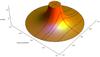 |
Fig. 1 Radial density profile of a model clump. The dashed lines show the density profile along various lines of sight (for different impact parameters p). |
2. The KOSMA-τ PDR model
A large number of numerical PDR codes is presently in use and an overview of many established PDR models is presented in Röllig et al. (2007)1. We use the KOSMA-τ PDR code (Störzer et al. 1996; Röllig et al. 2006)2 to numerically solve the coupled equations of energy balance (heating and cooling), chemical equilibrium, and radiative transfer. The main features of the KOSMA-τ PDR model are: a) spherical model symmetry, i.e finite model clouds; b) modular chemistry, which means, that chemical species can easily be added or removed from the network and the network will rebuild dynamically; c) isotope chemistry including 13C and 18O; and d) optimization toward large model grids in parameter space, allowing for example to build up any composition of individual clouds in order to simulate clumpy material (for details see Cubick et al. 2008). The KOSMA-τ results can be accessed on-line at: http://www.astro.uni-koeln.de/~pdr.
2.1. Model physics
Individual PDR-clumps are characterized by the total gas density n at the cloud surface, the clump mass M in units of the solar mass, the incident, isotropic far ultraviolet (FUV: 6 eV ≤ E ≤ 13.6 eV) intensity χ, given in units of the mean interstellar radiation field of Draine (1978), and the metallicity Z. We assume a density power-law profile n(r) = n0(r/Rtot) − α for Rcore ≤ r ≤ Rtot, and n(r) = const. for 0 ≤ r ≤ Rcore. The standard parameters are: α = 1.5, Rcore = 0.2 Rtot, roughly approximating the structure of Bonnor-Ebert spheres. Figure 1 shows the applied density structure. In Appendix D we describe how to compute mean column densities for spherical model results.
Excitation of the H2 molecule is computed by collapsing all rotational levels with the same vibrational quantum number into a corresponding, virtual v level. We then solve the detailed population problem accounting for 15 ground-state levels (v = 0 − 14) and 24 levels from the Lyman band as well as 10 Werner band levels. We assume that chemical reactions with the population of vibrationally excited H2 have no activation energy barrier to overcome. This is especially important for species such as CH (Röllig et al. 2007) and CH+ (Agúndez et al. 2010). The heating by collisional de-excitation of vibrationally excited H2 is calculated from the detailed level population. Photo-electric heating is calculated according to Bakes & Tielens (1994). Overall, we account for 20 heating and cooling processes. For a detailed description see Röllig et al. (2006) and Röllig et al. (2007). All model results in this paper are for single-clump models without contribution from interclump gas and without clump superposition.
2.2. Model chemistry
In KOSMA-τ we solve pure gas-phase steady-state chemistry with the exception of H2 forming on grains (Sternberg & Dalgarno 1995). It relies on the availability of comprehensive databases of chemical reaction rate coefficients. Today a few databases are publicly available, such as UDfA3 (Woodall et al. 2007), the Ohio database OSU4, and the NIST Chemistry Webbook5. There are also efforts to pool all available reaction data into a unified database (KIDA: KInetic Database for Astrochemistry)6.
In the following we use UDfA06. Retrieved at the 09/29/2009 the database consists of 4556 reaction rates, involving 421 chemical species (420 species + electrons). 34 of these reactions are present with 2 or 3 entries, valid in different temperature ranges (Röllig 2011). All species in UDfA06 are composed of the main isotopes only.
2.2.1. Isotopization
In order to calculate chemical reactions involving different isotopologues, i.e. molecules that differ only by their isotopic composition, it is necessary to extend the chemical reaction set. For example, reaction 1 in UDfA06:
 becomes
 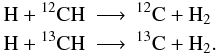 We developed a software routine to automatically implement isotopic reactions into a given reaction set7. A similar automatic procedure was used by Le Bourlot et al. (1993); Le Petit et al. (2006). We applied our routine to the UDfA06 reaction set, but it can be applied to any given set of chemical reactions. The routine features are:
-
inclusion of a single 13C and a single 18O isotope (multipleisotopizations are neglected in this study);
-
UDfA often does not give structural information, for instance C2H3 does not distinguish between linear and circular configurations (l-C2H3 and c-C2H3). In such cases we consider all carbon atoms (denoted by Cn) as indistinguishable. However, if structure information is provided we account for each possible isotopologue individually:
-
molecular symmetries are preserved, i.e. NC13CN = N13CCN, but HC18OOH ≠ HCO18OH;
-
functional groups like CHn are preserved (see also Woods & Willacy 2009);
-
when the above assumptions are in conflict to each other we assume minimal scrambling, i.e. we choose reactions such, that the fewest possible number of particles switch partners;
-
we favor proton/H transfer over transfer of heavier atoms;
-
we favor destruction of weaker bonds.
In Appendix A we describe in detail how isotopologues were introduced into the chemical network. The rescaling of the newly introduced reaction rates is described in Appendix B8.
2.2.2. Choice of the chemical data set
Some data sets, e.g. OSU, are more relevant for the cold ISM while others, for instance by including reactions with higher activation energy barriers, are better suited to describe the warm ISM. Consequently, the results of chemical model calculations may differ significantly depending on the applied chemical data set. Reactions that can be found in different chemical sets can have significantly different rate coefficients among the various sets. Even very prominent reactions, such as the photo-dissociation of CO (from now on we will omit the isotopic superscript when denoting the main isotope) are listed with very different rate coefficients: UDfA06 gives an unshielded rate coefficient of 2 × 10⁻¹⁰ s-1, OSU and KIDA give 3.1 × 10⁻¹¹ s-1. This is a huge difference and will lead to a significantly different chemical structure of a model PDR. It is not the purpose of this paper to perform a detailed analysis of how the choice of a chemical data set affects PDR model results. However, we show in Appendix C how the (isotope-free) chemistry of the main species discussed later in this paper changes for three different chemical sets. For a similar discussion see also Wakelam et al. (2012).
2.2.3. Isotope exchange reactions
In this frame reaction (C 1) turns into two reactions, one for the forward, one for the back reaction, where both have the value of α (the rate coefficient for reaction (C 1) is k(C 1 →) = 4.42 × 10⁻¹⁰(T/300 K)-0.29), but where the back reaction is suppressed by the factor exp(−γ/T) with γ = 35 K. Watson et al. (1976) proposed that carbon isotope transfer between interstellar species can occur as a result of reaction (C 1). At low temperatures, reaction (C 1) transfers 13C isotopes from 13C + −→ 13CO, enhancing the abundances of 13CO and 12C+. This reaction needs three main ingredients: sufficient amounts of 13C+ and CO and temperatures well below 100 K. In the PDR context, reaction (C 1) is especially interesting, because in the outer transition regions, where CO is still strongly dissociated, the 13C+ abundance is very large while 13CO is very rare. Even small numbers of 13CO products from reaction (C 1) will have a significant influence on the total 13CO abundance and thus on the [CO]/[13CO] ratio. Vice versa, 13C+ will be depleted strongly, increasing [C+]/[13C+]. Smith & Adams (1980) measured another isotope-exchange reaction:
 (C 2)with less effect on the hotter parts of the PDR, due to the low differences in back and forward reaction rates at higher temperatures. Langer et al. (1984) tabulated reaction rates and reaction enthalpies for the various isotopic variants of reactions (C 1) and (C 2) and we use their values in our calculations. Slightly different reaction rate coefficients are also given by Liszt (2007) and Woods & Willacy (2009) but the differences are small.
3. Application
3.1. Model parameter grid
We test the outcome of the isotopic network under various conditions by computing a large grid of models spanning the possible parameter space. Our chemical network consists of 198 species, involved in a total of 3250 reactions. We did not include 18O into the chemistry here.
We separate the model parameters into two sets: fixed and variable. The fixed parameters determine the fundamental physical and chemical conditions for the model clouds, e.g. gas density profile parameters α and Rcore/Rtot, cosmic ray ionization rate ζCR of molecular hydrogen elemental abundances Xi, metallicity, and dust composition. The variable parameters compose the final model parameter grid. A common set of variable parameters is: total surface gas density n0 = n(Rtot) = nH + 2nH2, cloud mass M, and ambient FUV field strength χ in units of the Draine field (Draine 1978). For a given density law, α and fc = Rcore/Rtot, the total cloud radius ![\hbox{$R_\mathrm{tot}=5.3\times 10^{18} \sqrt[3]{M/n}$}](/articles/aa/full_html/2013/02/aa20130-12/aa20130-12-eq50.png) cm and the maximum (radial) column density Nmax = 4.7nR cm-2 (see also Appendix D).
cm and the maximum (radial) column density Nmax = 4.7nR cm-2 (see also Appendix D).
Overview of the most important model parameter.
For the present study we varied the clump parameters n0, M, χ and kept all other parameters constant. Table 1 gives an overview over the used parameters. We assume a dust composition according to Weingartner & Draine (2001) (entry 7 in their Table 1, which is equivalent to RV = AV/EB − V = 3.1). From the extinction cross section of each dust component we compute an average, effective FUV dust cross section per H σD. For a given total gas column density Ntot, then follows: τFUV = NtotσD, and AV = σDNtot1.086/3.08. The term in the denominator corrects from visual to FUV extinction. Note, that the elemental abundances of carbon show an elemental ratio (ER) of 67, close to the average ratio in the local ISM (Sheffer et al. 2007). We computed 168 models. The computation times per model range from 36 to 930 min with a median of 100 min9.
3.2. Structure of the C+/C/CO transition
The chemical stratification of C+–C–CO, the carbon transition (CT), is a well known signature of PDR chemistry (e.g. Hollenbach & Tielens 1999). The stratification is the result of a number of competing formation and destruction processes like photo-dissociation, dissociative recombination, and others. Photo-dissociation of CO by FUV photons is a line absorption process, and as such subject to shielding effects (van Dishoeck & Black 1988). Numerically, this can be described by shielding factors that depend on the column densities of dust and of all species that absorb at the frequency of the line. The shielding factor multiplicatively enters the photo-dissociation rate, i.e. describes the reduction of the photo-dissociation through the line absorption. In the case of carbon monoxide the shielding depends on the columns of H2 and CO (e.g. van Dishoeck & Black 1988; Lee et al. 1996; Warin et al. 1996; Visser et al. 2009)10. The self-shielding of the CO leads to stronger photo-dissociation of the rarer isotopologues at a given AV11. This is also shown in Fig. 2. Because of the lower column density of 13CO, with respect to the main isotopologue, it takes a larger cloud depth for 13CO to become optically thick than it takes for CO. From Fig. 2 it can be seen that photo-dissociation of 13CO is still strong at AV ≈ 0.3 where CO is already optically thick.
The physical conditions, such as density structure and FUV illumination, determine where the CT is situated. For the purpose of this paper we define CT as the position in a cloud where n(C + ) = n(CO). The details of the C+–C–CO structure are changed by various effects. C+ remains the least affected species. At the outside of the cloud photo-ionization turns basically all carbon into C+. The strength of the FUV field and the attenuation by dust determine the depth where recombination dominates over ionization and the C+ abundances decreases. Carbon now becomes distributed between numerous species, but once shielding of CO becomes effective, usually at AV ≳ 1, the large majority of all carbon atoms is bound into carbon monoxide. Both species, C+ and CO, are quite insensitive to changes in the chemistry or the temperature structure, at least in cloud regions where they dominate the carbon population. However, in regions where they represent only a minor fraction of all carbon species, their chemical structure may depend sensitively on details of the cloud chemistry and physics. For example, increasing the H2 formation efficiency on hot dust grains, i.e. at low AV, increases the corresponding H2 formation heating efficiency, leading to higher gas temperatures in these cloud parts. This can produce an increase of the CO population in the hot gas and consequently produce strong emission of high-J emission (Le Bourlot et al. 2012; Röllig et al. 2013). The same effect can also positively affect the abundance of light hydrates, such as CH+ and CH, which are primarily formed in these regions.
Atomic carbon is the species that is probably most affected by changes in the chemistry and physics, because it is involved in the chemistry of C+ as well as CO and chemically constitutes a transitional species. It is the major carbon species, that is least understood. Observations and model predictions of the spatial distribution of C show big differences. The classical C+ − C − CO stratification, with C being sandwiched between its two big brothers is hardly observed at all. Instead, atomic carbon shows a widespread distribution that remains to be understood (e.g. Kramer et al. 2004, 2008; Mookerjea et al. 2006, 2012; Röllig et al. 2011).
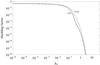 |
Fig. 2 CO shielding factors12 of a model clump with the following model parameters: n0 = 105 cm-3, M = 100 M⊙, χ = 10 (CO: solid line, 13CO: dashed line). |
3.3. Cloud fractionation structure
Unfortunately it is impossible to discuss the fractionation for all species from our chemical dataset so that we focus on a few molecules of particular astronomical interest. A complete coverage of the fractionation ratio (FR) for the selected species in our model grid is presented in Appendix E.
3.3.1. C+ and CO
Figure 3 shows the chemical structure of the main carbon species in the model clump. Solid lines show the main isotopologues, dashed lines the 13C variants.In the outer parts of the clump, most of the carbon is in the form of C+. The CT for the model shown in Fig. 3 is at AV ≈ 0.2 where the CO photo-dissociation rate has dropped sufficiently in order to build large quantities of CO, which leads to a steep decline in n(C + ) and n(C). In Fig. 4 we show the corresponding FR of the species from Fig. 3. We note a number of features:
- 1.
the FR of C+ is always larger than or equal to the ER., i.e. 13C+ is always under-abundant with respect to C+;
- 2.
the FR of C+ equals the ER at low AV;
- 3.
the FR of C+ increases significantly at large AV;
- 4.
the FR of CO is always smaller or equal to the ER except for conditions described in Sect. 3.3.2;
- 5.
the FR of CO deviates the strongest from the ER at low AV and equals the ER at large AV;
- 6.
the FR of C and HCO+ show mixed behavior.
 and destruction via the fractionation reaction. Dominance of reaction (C 1) automatically leads to fractionation, in this case to C+ enrichment relative to 13C+. The absolute magnitude of the FR is controlled by the He+ abundance which is a direct result of the cosmic ray ionization rate. In Fig. 4 this can be seen by the roughly constant FR of C+ deep inside the cloud. The same qualitative behavior is visible for all other model parameters in our model grid. Only the particular position, width and height of the FR peak of C+ varies with density and FUV field strength. Woods & Willacy (2009) find the same fractionation behavior in their protoplanetary disk model calculations. At the surface C+ is not fractionated while at large depths they find FR > ER.
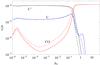 |
Fig. 3 Chemical structure of a model clump with the following model parameters: n0 = 105 cm-3, M = 100 M⊙, χ = 10. (main isotopologue: solid line, 13C isotopologue multiplied by ER = 67: dashed line). |
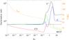 |
Fig. 4 Fractionation structure of the same model clump as shown in Fig. 3 (solid lines: fractionation ratios n(X)/n(13X), dashed line: kinetic gas temperature (right axis). |
The fractionation of CO is different because a second isotope-selective process is at work, the shielding of CO and 13CO from FUV photons. We would expect that if photo-dissociation was the dominant process, i.e. if 13CO photo-dissociation was relatively stronger than the photo-dissociation of the main isotopologue, then this would result in FR(CO) > ER. This is not the case for any model clump in our calculations. It happens in thinner clouds with n < 102 cm-3 as discussed by Liszt (2007). All models show a FR(CO) < ER indicating that the FR is dominated by the chemistry. I.e. by reaction (C 1) which can only produce FR < ER. Exceptions to this behavior are discussed in Sect. 3.3.2.
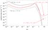 |
Fig. 5 Reaction rates for the same model clump as shown in Fig. 3 (photo-dissociation of CO: black, solid; 13CO: black, dashed; back and forth reaction rates in reaction (C 1): red). |
This is also visible from Fig. 5, where the destruction of CO (black, solid line) and 13CO (black, dashed line) via photo-dissociation is compared to the respective formation via reaction (C 1) (red lines). For CO photo-dissociation is the major destruction process until AV > 0.1. Then chemical destruction by the fractionation reaction takes over. Formation via the fractionation reaction is not the dominant formation channel of CO for most of the clump. Only for the small AV range of 0.1 ≤ AV ≤ 0.6 CO formation is dominated by the fractionation reaction. This is different for 13CO where destruction via photo-dissociation is weaker than formation by reaction (C 1) throughout the clump. Both, formation and destruction of 13CO is governed by reaction (C 1) (both red lines in Fig. 5). At AV > 2 electron recombination with H13CO+ becomes the main formation channel. Hence, for the whole low AV part of the clump, the 13CO abundance is controlled by the chemical fractionation reaction and accordingly, 13CO is significantly enriched relative to CO.
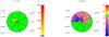 |
Fig. 6 Fractionation structure as function of relative clump radius r/Rtot for n = 103 cm-3 and M = 1 M⊙. Each sector corresponds to a different χ value. The FR is color coded, ratios within ± 10% of the ER are shown in green. Left panel: FR of C+, the color scale goes from 0 to 2000. Right panel: FR of CO, the color scale goes from 0 to 100. |
Figure 6 compares the FR of C+ (left panel) and CO (right panel) for n = 103 cm-3 and M = 1 M⊙. Each sector in the figure corresponds to a different FUV intensity χ. The FR, as function of the relative clump radius r/Rtot, is color coded, ratios within ± 10% of the ER are shown in green. Figure 6 gives a visual summary of the analysis above. The pie chart representation visualizes the relative contribution of the abundance profile at different radii of our spherical clumps to the integrated clump ratio. At n = 103 cm-3, fractionation of C+ only occurs deep inside the clump, while CO shows most fractionation further out. However, we also note, that for higher values of χ, the cloud is so hot that no fractionation occurs any more. The stronger the FUV intensity the deeper the dominance of the photo-dissociation of CO. No shielding or selective photo-dissociation can yet take place and the FR equals the ER. However, in case of n = 103 cm-3 and χ ≥ 102, CO can not be shielded efficiently and most of the carbon is locked in its ionized form. This is different for higher densities.
The situation at higher gas density is presented in Fig. 7. The fractionation of C+ is much more prominent and dominates a much larger clump volume compared to lower densities. As explained above, cold (T < 100 K) C+ is always fractionated with FR ≫ ER. This is true for the entire parameter grid. CO on the other hand, requires CO and sufficient 13C+ to become fractionated. These conditions are only met in a limited radius range, that is pushed to larger depths if χ increases. Deeper inside and further outside, the FR of CO equals the ER.
The effect of different clump masses is easier to understand. Adding mass is effectively equivalent to adding shielded, cold material to the clump, since it approximately requires a constant column of gas to attenuate the FUV radiation. Once this column is reached any additional material will be shielded and therefore located in the center of the clump. The appendix gives sector plots such as Figs. 6 and 7 for the full parameter grid.
As an additional effect, the 13CO recombination occurs at lower values of AV than the recombination of the main isotopologues, despite the lower shielding capabilities of 13CO compared to CO. This is true for all models in our parameter grid. Across our parameter grid, the CT of the main isotopologue occurs at a log (NCO) = 15.8 ± 0.4, while for the 13C variant (13CT) log (NCO) = 15.4 ± 0.4. The difference between both is smallest for models where photo-dissociation is more important, i.e. for larger values of χ. The comparison of the CO column density at the CTs of CO and 13CO for all models in our parameter grid is shown in Fig. 8. The colors of the data points represent the FUV field strength χ of the respective model.
The resulting impact on the column densities is shown in Fig. 9. Each symbol represents the column density ⟨ N(CO) ⟩ / ⟨ N(13CO) ⟩ of a model clump with given density n, mass M, and FUV irradiation χ (clump column densities are defined in Appendix D). Clumps with low CO column densities deviate most from the ER. Measurements of the column density ratio N(CO)/N(13CO) are usually performed on diffuse or translucent clouds and thus naturally confined to a low N(CO) regime.
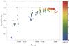 |
Fig. 8 Comparison of the AV,12CT and AV,13CT, i.e. the AV, where n(C + ) = n(CO) and |
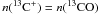
The low column density region of Fig. 9 is roughly consistent with UV absorption-line observations by Sonnentrucker et al. (2007). For translucent clouds they found an anti-correlation of ⟨ N(CO) ⟩ / ⟨ N(13CO) ⟩ with ⟨ N(CO) ⟩ in the range of 1014 cm-2 ≤ ⟨ N(CO) ⟩ ≤ 1016.5 cm-2. Liszt (2007) found 15 < N(CO)/N(13CO) < 170 with a tendency for the ratio to decline for higher column densities and a total CO column densities of a few 1016 cm-2 from Galactic CO absorption and emission at 1.3 and 2.1 mm wavelengths for clouds with a total CO column density N(CO) ≤ 1016 cm-2. Sheffer et al. (2007) showed, that UV data toward diffuse/translucent lines of sight can give 0.5 ≤ FR(CO)/ER ≤ 2.
Clumps with stronger FUV fields show almost no fractionation, either because the molecular inner parts are so small that the gas temperatures throughout the clump are too high or because fractionation only affects the CO at the outer clump regions but not the bulk of the CO gas. For sufficiently large CO column densities, the column density ratio of CO/13CO turns out to be a relatively good tracer of the elemental abundance ratio of a given cloud.
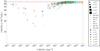 |
Fig. 9 Scatter plot of the mean column density fractionation ratio vs. the mean column density of the main isotopologue of CO/13CO of the whole parameter space. The model parameters n, M, and χ, are coded as size, shape, and color of the respective symbols. The red line denotes the model elemental abundance [12C]/[13C] = 67. |
The fractionation of the column density ratio of C+ is shown in Fig. 10. The lower FUV models show the largest FR while the models with very large FUV fields have a FR = ER. Models with low density show a much weaker fractionation (see also Fig. E.1) because the molecular part of the low density clouds contributes less to the total C+ column density. Increasing the model density (larger symbols in the figure) for given model mass and FUV illumination moves the models in Fig. 10 to the top left because larger densities lead to a stronger shielding of the gas from the FUV and therefore a CT closer to the clump surface. Consequently, the total C+ column density is decreased. On the other hand, the larger amount of cold CO gas acts in favor of the stronger C+ fractionation. However, these strongly fractionated model clumps show the lowest C+ column density making observations difficult. Observability will be further discussed in Sect. 3.4.
As an additional consequence, when keeping density and FUV constant, the FR of C+ is proportional to the clump mass. Increasing the clump mass leads to an increased FR, moving model points, visible as different symbols in Fig. 10, to the top right.
3.3.2. High density conditions with FR(CO) > ER
For typical molecular cloud conditions isotope-selective photo-dissociation is never strong enough to keep 13CO photo-dissociated while CO is already recombined. If isotope-selective photo-dissociation was dominating the CO chemistry one would obtain FR > ER, like it is found e.g. in diffuse clouds Liszt (2007). For special conditions, particularly for densities of n ≥ 106 and sufficient FUV illumination, FR > ER is still possible across a limited AV range. Figures 11 and 12 show the density and fractionation structure of such a clump. CO shows a first, relatively strong abundance peak at AV = 0.6, before the CT. The gas temperature at this AV is around 600 K. At this part of the clump, the FR of CO is higher than the ER. Closer examination of the parameter reveals that similar behavior can be found for models with n ≥ 106 and χ ≥ 104 (compare Fig. E.3).
Detailed chemical analysis of these models shows that FR > ER occurs at significantly lower cloud depth than the CT (see Fig. 11). The already mentioned CO abundance peak results from dissociative recombination of HCO+, which is effective in hot gas (Sternberg & Dalgarno 1989) and gives rise to the CO peak before the CT. At these cloud depths HCO+ itself is primarily formed by collisions of HOC+ and CO+ with H2 (CO+ forms through C+ + OH −→ CO+ + H and HOC+ has two main formation reactions: C + + H2O −→ HOC + + H and CO+ + H2 −→ HOC+ + H).
The maximum CO abundance in this peak strongly increases with the total gas density. Even so, we have not yet reached the CT, the total CO column density from the cloud’s edge to that peak position can already reach values ≳ 1015 cm-2, which is sufficient for self-shielding (van Dishoeck & Black 1988). Any CO self-shielding will be stronger for the main isotopologue than for 13CO and if photo-dissociation is the main destruction process for both isotopologues than the stronger shielding of CO can give rise to FR > ER. If the destruction of 13CO is controlled by reaction (C 1) than FR ≤ ER.
To understand which conditions can lead to FR > ER we balance the main formation and destruction processes of 13CO. We already noted that formation via dissociative recombination of HCO+ is a general requirement, otherwise CO self-shielding will not be effective. A second possible formation route is by the isotope exchange reaction (C 1). Destruction can be either via the back reaction (C 1) or by photo-dissociation. The gas temperatures are high enough to neglect the energy barrier of the back reaction and assume k(C 1 →) ≈ k(C 1 ←). The rate coefficient for dissociative recombination of HCO+ is k(DR) = 2.4 × 10⁻⁷(T/300 K)-0.29 s-1 cm3, and ζ13 is the photo-dissociation rate of 13CO. Hence 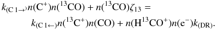 (1)With n(CO) = FR × n(13CO), n(e − ) ≈ n(C + ) ≈ 1.2 × 10⁻⁴ntot, and
  follows
 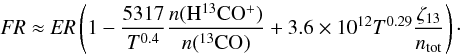 (2)The last two terms in parentheses compete in changing the FR relative to ER. In the relevant cloud regime, each term lies between ≈ 0.1 − 10, depending on the detailed conditions, and FR(CO) can increase to ≈ 80 − 100.
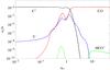 |
Fig. 11 Fractionation structure of the very dense model clump. The model parameters are n = 107 cm-3,M = 0.01 M⊙,χ = 105. (Main isotopologue: solid lines, 13C isotopologue multiplied by ER = 67: dashed lines.) |
We emphasize, that this behavior is not just a simple competition between chemistry and photo-dissociation as Liszt (2007) described for diffuse clouds. A FR > ER in PDRs is the result of a local, chemically induced, dominance of the photo-dissociation of 13CO over its chemical destruction. Only for 106 ≤ n ≤ 107 cm-3 and 104 ≤ nχ ≤ 106 are the conditions such that in a narrow AV range isotope-selective photo-dissociation leads to FR > ER.
3.3.3. C
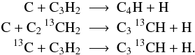
From Figs. 4 and 13 we see that the FR of C has a small regime at low AV and low FUV intensities where FR < ER, while under all other conditions the FR ≥ ER. The FR(C) starts to peak at the rise of FR(C+) followed by a dip where CO turns to the ER and by a second peak at the declining flank of FR(C+). Until AV < 5 − 10 atomic carbon is dominantly formed through one of the following reactions: 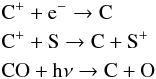 while destruction occurs mainly via photo-ionization. As discussed, the FR of CO and C+ behave oppositely in distinct cloud depths; FR(CO) ≤ ER, mainly in outer layers, while FR(C+) ≥ ER, somewhat deeper in.
At low AV both isotopic variants of atomic carbon will be dominantly formed from the recombination of their ionized forms and C will share the FR of C+. This is visible as first peak in FR(C). The weaker shielding of 13CO and the strong fractionation of C+ makes photo-dissociation of 13CO the major formation reaction for 13C for AV > 0.2. The isotope-selective shielding drives the FR of C toward lower values and gives rise to the dip in the curve in Fig. 13. The magnitude of this diminishment depends on the differences in the shielding of 12CO and 13CO and the cloud depth where the shielding is still weak. If this difference is still significant when FR(C) reaches its first peak it can push the FR to values smaller than the ER.
For AV > 0.2, until FUV shielding becomes strong, 13CO + hν will be one order of magnitude faster than any of the other formation reactions while photo-dissociation of 12CO will never be the dominant formation reaction. At AV > 1, FR(CO) = ER and the FR(C) will increase again. Charge transfer between C+ and S becomes the major formation reaction and consequently, C will share the FR of C+. At very large cloud depths cosmic-ray-induced photo-dissociation of CO becomes a main formation reaction together with charge transfer between C+ and SO for C and charge transfer between N+ and 13CO for 13C. As a result, the FR(C) will slowly decrease with increasing AV.
3.3.4. CH+ and CH
Figure 14 summarizes the dominant formation and destruction channels of the discussed hydrocarbons. The arrows denote the primary reaction channels for CH+, CH , and CH
 (left panel) and for CH (right panel) across the model clumps. Figure 15 shows the FR of C+, CH+, CH, CH, and CH and Fig. 18 shows the abundance profile of hydrocarbons and their respective isotopologues.
The reaction C + + H2 + ΔE −→ CH + + H requires an activation energy of ΔE = 4600 K, but collisions with vibrationally excited  allow to overcome the barrier (Röllig et al. 2007; Agúndez et al. 2010). At the edge of the cloud, CH+ is primarily produced from C+ colliding with excited, molecular hydrogen. At AV ~ 10-3, the proton exchange reaction C + + CH −→ CH + + C together with ionization of CH become the main formation reactions. In those two regimes, the FR is controlled by C+ (see also Fig. 15). At AV ~ 1 the main formation occurs via collisions of C with HCO+ or H.
Under very high density and very low χ conditions, C+ will be less abundant than C throughout the clump. As a result the dip between the two peaks visible in the FR(CH+) in Fig. 15 becomes much more prominent and can reach values below ER. This is visible in Fig. E.6.
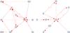 |
Fig. 14 Chemical network of the dominant formation and destruction channels for: left panel: CH+, CH |
The formation of CH originates at C+. Successive collisions with H2 form the chain:  At the end of the reaction chain dissociative recombination leads to CH and CH2. At low AV, CH can also be formed from C, at high AV it forms via dissociative recombination of HCS+. The reaction paths to CH (in order of cloud depths where they dominate) then are:
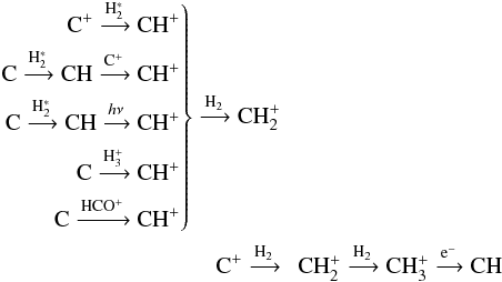
 From Fig. 15 and from the above chain of reactions it is obvious, that the fractionation ratio of C+ will be handed down through the chain, unless other carbon species become involved. This is the case for CH. At very low AV where the formation via
  is most important, and the FR is closely related to C which mostly equals the ER under these conditions. Once the FR of C+ starts increase, it will affect the fractionation of all the related
  and consequently that of CH.
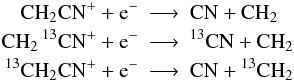
Deeper in the cloud the same happens along a different chemical track. Recombination of CH and of HCS+ (once AV > 3) are the main formation reactions for CH. The chemical chain C+, C2N+, C2, CS+, HCS+, CH shares a common behavior of the FR (see also Fig. 15). As a side remark we would like to emphasize this chain as a good example of how the chemical networks of different elements, sulphur and nitrogen in this case, are mixed. Consequently it is important to include both networks to correctly compute the carbon chemistry.
 |
Fig. 15 Fractionation structure of light hydrocarbons for n0 = 105 cm-3, M = 100 M⊙, χ = 10 (green: FR(C), red ER). |
In Figs. 16 and 17 we show the FR of CH+ and CH respectively. The FR(C+) deviates from the ER only at larger values of AV and column densities of species whose FR depends on FR(C+) will only be affected if these deeper cloud regions contribute significantly to their total column density. For CH+ this is the case for the same parameters where also C+ is fractionated and Fig. 16 shows their close chemical relationship. Deviations from the ER occur only for the low χ models with sufficient total column densities, similar to C+ (see Fig. 10).
The weak deviations of the FR(CH+) from the ER is consistent with observations. Centurion et al. (1995) found a mean value of the CH+/13CH+ column density ratio of 67 ± 3 for five lines of sight, very close to the interstellar ER. Casassus et al. (2005) report an average ratio of 78 ± 2 from measurements along 9 lines of sight. Recent absorption-line observations by Ritchey et al. (2011) along 13 lines of sight through diffuse molecular clouds confirm a FR(CH+) close to the ambient ER. They report total column densities of CH+ of a few 1013 cm-2.
CH remains abundant approximately until AV approaches unity. As a consequence, a larger fraction of its total column density will be affected be the fractionation. This is visible in Fig. 17. Above a mean column density of 1013 cm-2, all models show an enhanced FR. Because of the strong coupling to FR(C+), weaker FUV models tend to have the strongest fractionation. Therefore, CH promises to be a good observational fractionation tracer as it combines enhanced FR with high column densities.
3.3.5. HCO+
The fractionation of HCO+ is special because it is affected by two processes acting in opposite directions. At very low AV HCO+ is formed by H2 collision with HOC+ and CO+. Both precursors are not fractionated, thus FR(HCO+) ≈ ER (see Sect. 3.3.2). A little deeper into the clump, the main formation reaction changes to CH + O −→ HCO + + e − , thus its fractionation indirectly depends on reaction (C 1). CH is strongly fractionated with FR > ER and passes down the fractionation to HCO+. This fractionation peak is seen in Figs. 4 and 19. With growing χ the peak is pushed to larger cloud depths. Once CO is sufficiently abundant, the reaction  takes over as dominant formation reaction and the FR approaches that of CO (compare with Fig. 7, right panel). At even higher values of AV the gas temperature becomes very low (T ≤ 10 K) and reaction (C 2) starts to dominate formation and destruction of HCO+ and pushes the FR significantly below the ER. In the appendix we show the FR of HCO+ over a significant portion of our model grid. The central cloud regime with FR < ER is visible in all clumps that are sufficiently shielded from the external FUV radiation.
In Fig. 20 we show the column density fractionation ratio of HCO+. Fractionation of HCO+ is strongest for clumps with large columns of cold gas, where reaction (C 2) can contribute strongly to the total H13CO+ abundance. Low mass and low density models have a FR equal to the ER or slightly higher. For a given density, the FR is largely independent of the model mass, which is consistent with the HCO+ and H13CO+ density profiles shown in Fig. 18 which show an increase for large AV and a roughly constant FR (see also Fig. 4). Hence, the FR of HCO+ is only marginally affected if the clump mass is increased. The model results show a strong correlation of the column density ratio with χ.
3.4. Emission line ratios
Even though column densities are no direct observables, they have to be derived from measured line strengths resulting from the full radiative transfer, including effects of a variable temperature of exciting collision partners and optical depths. However, the derivation of intensities requires numerous additional assumptions, such as collision rates, details of the geometry, assumptions on chemical and radiative pumping, and so on. Consequently, from a modellers perspective intensities have larger uncertainties than column densities. Therefore we only compute intensities for a selected subset of commonly observed species and transitions. Here, we directly compare the isotopic ratio of clump averaged line intensities (for definition see Röllig et al. 2006) which can be compared directly to observations. We always assume unity beam filling factor. The large number of possible line combinations prohibits a complete presentation. We give just a few examples to demonstrate that line ratios between various isotopologues can differ from the corresponding column density ratios.
Figure 21 shows the ratio of Tmb( [CII] )/Tmb( [13CII] ) with  (For 13C+ we summed over all hyperfine components.). While the column density ratio is larger than the ER for all model clumps the same is not true for the intensity ratio (IR). All models with χ > 100 show a IR < ER down to values of 38. Only models with very low χ and large densities have a IR > ER. For a given density and mass, the IR decreases with increasing χ, because of the larger optical thickness of C+ relative to 13C+. [13CII] observations of the Orion nebula by Stacey et al. (1991) show a very similar behavior and are consistent with our model predictions. They report line ratios between 36 and 122 with the highest optical depths
  belonging to the lowest line ratio of 36 ± 9 and low optical depths where ratios are high. Boreiko & Betz (1996) derive an intensity ratio of 46 in M42, consistent with an intrinsic ER of
  and an optical depth of [CII] of 1.3. For a given χ, the IR drops with decreasing density and increasing mass. Increasing the mass for a given χ and n will add cool, molecular mass. Provided that C+ is fractionated this will increase the FR as long as the [12CII] line remains optically thin and decrease the FR once it becomes optically thick (compare Fig. 21).
In the previous section we showed, that the column density ratio of CO/13CO is close to the ER of the clump for most of the parameter space. CO emission lines suffer much more from optical thickness effects than most other species. This is also shown in Fig. 22 where we plot the ratio of the integrated intensities of CO(1−0)/13CO(1−0). For most of the models, this ratio is between 1 and 10, much smaller than the ER. Quite a few models have intensities of the rarer isotopologue comparable to those of the main species.
The low mass, high density models show an increasing IR with χ, opposite to the high mass, low density models. This is a result of the CO abundance structure of these model (see Fig. 11). The lowest IR is shown at the highest model mass model (IR ≤ 2) while the highest IR belongs to models with the lowest mass. Both can be explained as optical depth effect. Models with n ≥ 107 cm-3 have an increasing Tmb(CO(1 − 0)) with χ and the IR increases for the lower mass models and decreases for the higher mass models. The latter results from high optical thicknesses while the former results from the emission of of very hot, strongly excited CO gas in the primarily ionized fraction of the clump.
In Fig. 23 we plot the intensity ratio of CO lines Tmb(CO(J → J − 1))/Tmb(13CO(J → J − 1)) as a function of J for models with M = 10 M⊙ and line intensities > 0.01 K km s-1. For the lowest transition, the ratio lies between 1 and 10 and approaches ER for high values of J, when both lines become optically thin. The J where the ratio reaches the ER increases with n and χ. For instance, models with n = 107 cm-3 and χ = 106 have a ratio of close to unity, until J > 10 and reaches ER at J ≳ 25, while models with the same density and χ = 103 reach ER already at J = 15. We find that either the CO lines are optically thick so that the IR is lowered below the ER or the 13CO is too weak to be detectable. Only in dense clouds the ER is observable. The CO IR is therefore not a good diagnostics of carbon fractionation.
3.5. Diagnostics
Finally, we studied several line ratios with respect to their diagnostic value for the local FR of CO and C+ as well as to the local ER. We already concluded that CH and HCO+ appear to be sensitive tracers of the FR. Lacking collision rate coefficients for CH we only calculated HCO+ (and H13CO+) intensities for our model clouds.
We selected transitions that are observable from the ground or through SOFIA (Stratospheric Observatory For Infrared Astronomy) and show at most moderate optical depths of a few. Figure 24 demonstrates how the emission line ratio Tmb( [CII] )/Tmb(H13CO + (1 − 0)) traces the column density FR of C+, C and CO. The figure reproduces the general trend of the FR as discussed in the previous sections. We find a clear dependence of the emission line ratios on the column density FR of C and C+, but not of CO. However, it is only partially applicable to observational data. All ratios above ~ 30 000 are practically not observable as they correspond to H13CO+ intensities below 10 mK km s-1. If we exclude models with line intensities < 0.01 K km s-1 the column density ratios of CO and C+ show much weaker variations so that the emission line ratio only traces the fractionation of atomic carbon in the observable intensity range. We have repeated this exercise for many other line ratios that are available through ground based and satellite observatories, and that are strong enough to be observable13. All three panels in Fig. 24 show a transition around an emission ratio of 102 − 103. This ratio corresponds to models with the highest Tmb(H13CO + (1 − 0)) ≈ 1 − 2 K km s-1 and FR(C) slightly below the ER. It requires χ = 104 − 105 and densities of n = 107 to reach these high values. Toward lower intensities, the models split into two branches: very high density models with n = 107 cm-3 and decreasing FR(C), and models with n = 106 cm-3, χ ≥ 100 and increasing FR(C). This parameter regime corresponds to model clumps with the highest [CII] emission, increasing with n and χ. Accordingly, the [CII]/H13CO+ intensity ratio can increase to very high values if the density and the FUV field are high enough, albeit with the visible transition.
 |
Fig. 23 Emission line ratio Tmb(CO(J → J − 1))/Tmb(13CO(J → J − 1)) vs. J for all models with M = 10 M⊙. Models with line intensities < 0.01 K km s-1 have been omitted. |
Figure 25 shows the result for the three ratios that seem to be suitable to trace the column density FR of C+, C, and CO individually. The left panel shows Tmb(13CO(2 − 1))/Tmb( [CI] 610 μm) on the x-axis and the CO column density ratio on the y-axis. The level energy of 13CO (2 − 1) is 16 K, while the [CI] line requires 24 K for excitation. Looking at the plot, we note, that any line ratio < 1 signals significantly fractionated CO column densities. Any emission line ratio higher than a few reflects a normal FR in the CO gas. All models with an emission line ratio smaller than ≈ 1 have n ≤ 104 cm-3 and will consequently host a small 13CO population but significant amounts of atomic carbon.
The middle panel plots the column density fractionation ratio of atomic carbon versus Tmb( [CII] )/Tmb(H13CO + (1 − 0)) (same as in Fig. 24, but excluding all model lines too weak to be detectable). The model results show a strong correlation between the FR and the emission line ratio. The black line in the plot corresponds to a least-squares-fit f = 51x0.043 with the emission line ratio x. The [CII] emission is strongest for low to intermediate densities while HCO+ is a typical density tracer. Both lines are typical PDR tracers, sensitive to significant FUV illumination. Consequently, a line ratio higher than 103 signals FR > ER. The corresponding points in the plot belong to models with n ≈ 106 cm-3 and χ ≥ 104. The points with a FR < ER correspond to models with even higher densities and somewhat lower χ.
The panel on the right side shows the C+ column density ratio plotted against Tmb(13CO(1 − 0))/Tmb( [CII] ). All models with a line ratio higher than 2 contain fractionated C+. We saw in Fig. 10 that the FR(C+) is strongest for low UV models with high densities. These models have weak C+ emission, usually smaller than a few K km s-1, while these conditions favor 13CO emission resulting in large line ratios.
 |
Fig. 24 Column density fractionation ratios plotted against the emission line ratio Tmb( [CII] )/Tmb(H13CO + (1 − 0)) for all models from our parameter space (blue: ER, red: ER ± 10%, dashed: ER ± 20%). The symbols follow the coding from Fig. 9. The gray areas denote the regime below a sensitivity limit of Tmb < 0.01 K km s-1. Left panel: N(CO)/N(13CO), middle panel: N(C)/N(13C), right panel: |

 |
Fig. 25 Column density fractionation ratios plotted against emission line ratios for all models from our parameter space. (blue: ER, red: ER ± 10 %, dashed: ER ± 20%). Models with line intensities < 0.01 K km s-1 have been omitted. The symbols follow the coding from Fig. 9. Left panel: N(CO)/N(13CO) vs. Tmb(13CO(2 − 1))/Tmb( [CI] 610 μm), middle panel: N(C)/N(13C) vs. Tmb( [CII] )/Tmb(H13CO + (1 − 0)), right panel: |
4. Summary
We present an update of the isotope chemistry used in our PDR model code KOSMA-τ. An automated routine was created to allow for the inclusion of isotope reactions into the chemical database files that are used in numerical PDR computations. This is combined with a proper rescaling of the new isotope reactions. We computed a large parameter grid of spherical PDR model clumps and investigated the effect of the isotope chemistry, particularly that of the isotope exchange reaction (C 1), on the chemical structure of the model clumps as well as on their emission characteristics.
In the transition from ionized carbon to carbon monoxide the fractionation ratio of C+ is always larger than the elemental ratio in the gas. Strong C+ fractionation is possible in cool C+ gas. However, this is only partly visible in the corresponding intensity ratios of the model clumps. Optical thickness and excitation effects produce intensity ratios between 40 and 400, strongly dependant on the model parameters.
In the dense (n ≥ 103 cm-3) gas, CO behaves differently and is never found with a fractionation ratio larger than the element ratio with the exception of a very limited AV range under very special parameter conditions. In the diffuse gas Liszt (2007) found qualitatively different behavior for n < 102 cm-3 and M > 103 M⊙. It turns out that isotope-selective photo-dissociation, the major process able to produce a FR>ER, is always dominated by the chemistry in the denser PDR gas. This also affects the depth at which the transition from C+ to CO occurs. The formation and destruction of 13CO is much stronger controlled by reaction (C 1). A direct consequence is that in all models in our grid 13CO is formed at smaller AV than CO despite the weaker shielding capabilities of the rarer isotopologue.
The fractionation of other species can be understood in terms of their formation history. If their major formation channel originates from C+ their FR is related to FR(C+). This is the case for many light hydrides, especially CH, CH, and CH. If the FR of the parental species is controlled by other reactions than (C 1) the behavior might change. Atomic carbon is a mixed case with a regime at lower AV where formation occurs mainly via recombination of C+ and a regime where it is chemically derived from CO and HCO+. Consequently, the FR(C) exhibits a mixture of both cases. At particular depths, CH+ might be formed from C. If that is the case the relation of its FR to FR(C+) breaks down until formation via a C+ route takes over again.
Our computations have shown that CH and HCO+ may be very sensitive tracers for chemical fractionation in PDRs. CH amplifies the FR of C+ and HCO+ amplifies the FR from CO in the CT. Both are abundant in the region where chemical fractionation plays a big role and suffer less from optical depth effects than their chemical progenitors.
We demonstrated that fractionation of the local densities not necessarily transforms into a fractionated column density. C+ is a prominent example. Fractionation of ionized carbon only takes part in cool C+ gas which in most clouds only makes up a small fraction of the total gas column. Only low FUV models are able to produce larger columns of cool C+ and will have a fractionated column density. CO behaves oppositely in that it requires warm CO in order to become fractionated. Again, this affects the column density only under certain conditions.
Finally, we provide diagnostics for the fractionation status of C+, C and CO through suitable emission line ratios. We showed that a line ratio of Tmb(13CO(2 − 1))/Tmb( [CI] 610 μm) < 1 signals a significant fractionation of the CO column density. The line ratio of Tmb( [CI] 610 μm)/Tmb(H13CO + (1 − 0)) has a power law dependence on the fractionation ratio of the column density of atomic carbon. The column density fractionation of ionized carbon is reflected in Tmb(13CO(1 − 0))/Tmb( [CII] ) > 2.
Online material
Appendix A: Isotopization rules
Usually, only the main isotopes are considered in astrochemical databases, despite the fact that many isotopologues have been detected in astronomical observations so far. We will describe here our efforts to include 13C and 18O isotopes into the chemical database. However, in this paper we will only discuss the scientific implications of carbon fractionation not going into the details of the 18O chemistry.
Usually, in a reaction formula like H + O2 −→ OH + O it is not possible to identify which oxygen atom binds with hydrogen. Both atoms in O2 are indistinguishable. This changes by including an isotope into a molecule. Now both atoms in O18O are distinguishable and we get:  Unfortunately, this becomes more complicated if the isotope can be placed in more than one spot. The main isotope reaction
  splits into 5 isotopic reactions
 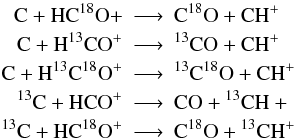 taking into account that the C=O binding is preserved (again we omit the isotopic superscript when denoting the main isotope). For more complex species the above scheme becomes much more complicated. Furthermore, the number of additional reactions is so large that it becomes difficult to perform the isotopization by hand, especially if one plans to update the chemical network regularly and manual isotopization is quite error-prone. We developed a software routine to automatically implement isotopic reactions into a given reaction set14. The routine features are:
-
inclusion of a single 13C and a single 18O isotope (multiple isotopizations are neglected in this study);
UDfA often does not give structural information, for instance C2H3 does not distinguish between linear and circular configurations (l-C2H3 and c-C2H3). In such cases we consider all carbon atoms (denoted by Cn) as indistinguishable15, i.e.
 However, if structure information is provided we account for each possible isotopologue individually:
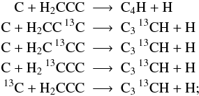
-
molecular symmetries are preserved, i.e. NC13CN = N13CCN, but HC18OOH ≠ HCO18OH;
functional groups like CHn are preserved (see also Woods & Willacy 2009), e.g.:
 but not:
-
when the above assumptions are in conflict to each other we assume minimal scrambling, i.e. we choose reactions such, that the fewest possible number of particles switch partners. For example:
 but not
  which would preserve the 13C=O bond but would require 5 particles to switch partners;
 we favor proton/H transfer over transfer of heavier atoms;

Appendix B: Rescaling of reaction rates
By introducing isotopologues into the chemistry we introduce many new reaction channels and we need to make sure that reaction rates are properly scaled. Unfortunately, not only the reaction rates for isotopologue reactions are unknown, we neither have information on branching ratios for reactions with several possible product channels. Thus, we assume equal probabilities for all branches, i.e. all isotopologue reactions possessing the same reactants but different products have their rate coefficient divided by the number of different product branches. For example:  with α being the fit coefficient from UDfA06 at T = 300 K and the number in parentheses indicates the decimal power. Introducing 13C and 18O into this reactions opens up additional channels:
  Assuming equal probabilities for different reaction branches is a strong assumption and the reader should keep in mind, that many of the introduced reactions might have different reaction rate coefficients with potentially strong impact on the solution of the chemical network. The isotope exchange reactions discussed in the following are a notable exception from this.
Appendix C: Influence of chemical data sets
To illustrate how the choice of the chemical data set affects the outcome of our astrochemical calculations we calculate our reference model for three different chemical sets: UDfA06 (Woodall et al. 2007), OSU (version osu_01_2009), and KIDA (version kida.uva.2011, Wakelam et al. 2012). To allow a consistent computation it was necessary to slightly alter the original data sets:
-
The formation of H2 on grain surfaces is calculated separately in KOSMA-τ and we removed the reaction H + H −→ H2 from OSU.
-
The same holds for the photo-dissociation of H2, we removed the reaction H2 + hν −→ H + H. KOSMA-τ explicitly calculates the H2 formation rate from the population of the (vibrational) v-levels (all rotational levels of one vibrational state summed, ground state v = 0 − 14, Lyman band 24 level + Werner band 10 level)
-
The unshielded CO photo-dissociation rate coefficient differs significantly among the three sets. We recomputed the unshielded photo-dissociation rate for a standard Draine FUV field using absorption cross sections available from http://home.strw.leidenuniv.nl/~ewine/photo/ and can confirm the value of 2 × 10⁻¹⁰ s-1 (van Dishoeck et al. 2006) from UDfA06. We replaced the corresponding α values in OSU and KIDA. For a discussion on differing photo-reaction rates see e.g. van Hemert & van Dishoeck (2008) and Röllig et al. (2013).
-
We replaced reactions with very large negative rate coefficients γ with a refitted expressions according to Röllig (2011).
-
KIDA uses the Su-Chesnavich capture approach to compute rate coefficients for unmeasured reactions between ions and neutral species with a dipole moment (Woon & Herbst 2009). Their formalism is incompatible with KOSMA-τ and we replace the corresponding 1877 reaction rate coefficients with a new set of rate coefficients α,β, and γ, suitable for the Arrhenius-Kooij formula α(T/300K)βexp(−γT), which are fitted such that they approximate the original rates between 10 and 1000 K.
-
For species where KOSMA-τ does not distinguish between linear and cyclic isomeric forms we consider all species only in terms of their molecular formula, e.g. C3H instead of l−C3H and c−C3H.
In Fig. C.1 we show the relative abundances of C+, C, and CO for model calculations with n = 105 cm-3, M = 1000 M⊙, and χ = 10 using different chemical data sets: UDfA06 (solid lines), OSU (dashed lines), KIDA (dotted lines) and the resulting range of gas temperatures. All three sets give the same chemical structure but with slight variations in the abundance profiles. The biggest difference is a higher CO abundance of OSU and KIDA at very low values of AV (factor 2 − 3 at AV = 0.01). This also leads to a carbon transition from C+ to CO at slightly lower values of AV compared to UDfA. Overall, the chemical structure of the main carbon species is comparable, particularly the effect on the total column density is small. The similar chemical structure and the almost identical gas temperatures around the carbon transition will result in a consistent fractionation behavior of the three species across all three chemical sets.
 |
Fig. C.1 Chemical structure of a model clump with the following model parameters: n0 = 105 cm-3, M = 100 M⊙, χ = 10 (UDfA06 (solid), OSU (dashed), KIDA (dotted). The gray shaded area shows the gas temperature spanned by the three models calculations. |
Figure C.2 shows how the different chemical sets influence the chemistry of HCO+, CH, and CH+. The differences are larger than those in Fig. C.1. UDfA06 produces a significantly higher CH abundance in the outer layer of the cloud, at some positions by a factor of 10 higher than OSU. However, we discussed earlier that fractionation of CH is the result of C+ fractionation. We do not expect any significant deviations in the fractionation ratio (FR) of C+) for the three chemical sets, hence the effect on the FR(CH) should be weak. The same should be the case for CH+ which shows even smaller differences for the three chemical sets. HCO+shows the same abundance in the cloud center, but some significant differences for AV < 1. This could lead to different fractionation behavior at these parts of the cloud when using different chemical sets. It is unlikely that this leads to observable effects because of the 100 times lower HCO+ abundance with respect to the center of the cloud and the respective weak influence on the total column density.
Appendix D: Spherical model context
D.1. Cloud radius
The model primarily computes radius dependent quantities. For a given density law, i.e., values α and fc = Rcore/Rtot, the total cloud radius Rtot (in cm) can be calculated from n0 (in cm-3) and M (in M⊙) using ![\appendix \setcounter{section}{4} \begin{equation} \label{rtot} R_\mathrm{tot}=6.57\times 10^{18} \sqrt[3]{-\frac{(\alpha -3) M f_c^{\alpha }}{n_0 \left(3 f_c^{\alpha }-\alpha f_c^3\right)}}\,\mathrm{cm}. \end{equation}](/articles/aa/full_html/2013/02/aa20130-12/aa20130-12-eq263.png) (D.1)For α = 3/2 and fc = 0.2 this reduces to cm.
(D.1)For α = 3/2 and fc = 0.2 this reduces to cm.
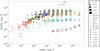 |
Fig. C.3 Mean CH column density versus H2 column density (color/shape coding same as Fig. 9). Observational results are plotted as colored points (red: Sheffer et al. 2008; green: Rachford et al. 2002; olive: Magnani et al. 2005; black: Qin et al. 2010; brown: Magnani et al. 2006; orange Gerin et al. 2010; blue Suutarinen et al. 2011). The two lines are the CH − H2 relations from Mattila (1986) (red) and Qin et al. (2010) (black). |
D.2. Column density
The general expression for the maximum (radial) column density16 is  (D.2)that is Nmax = 4.7nR cm-2 for α = 3/2 and fc = 0.2.
However, they are not observables. Observations always yield an projected, beam-convolved figure. We describe them in terms of measurable column densities.
In the framework of spherical model clouds, column densities differ depending on where we look at. To get a position-independent measure for the column density of a given species i, we calculate the average column density for the whole clump  (D.3)When referring to model column densities we always mean a clump averaged column density according to Eq. (D.3). This definition assumes that observations always cover whole clumps. This is equivalent to the traditional description of beam-filling factors for the observation of spatially unresolved clumps, i.e. we assume that we have (typically many) unresolved clumps within the telescope beam. In that sense, the fractionation of the column density is always the result of a convolution of the fractionation structure with the absolute abundance profile.
D.3. CH column densities
Modelling the formation of the light hydrides, such as CH+ and CH, still poses a challenge to chemical models. In Fig. C.3 we plot the mean CH column density versus the total mean column density of the respective clump. The colored dots are observations from absorption and emission line measurements. The red and black lines are simple parametrized models to describe the column density (Mattila 1986; Qin et al. 2010). We note, that the column density splits into two distinct regimes with significantly different behavior. Diffuse clouds with total column densities below 1021 cm-2 show a steeper slope than denser clouds, where the CH column density appears to approach a limit of about 1015 cm-2. This behavior is approximately reproduced by the model calculations. The column densities in our model are consistent with values for TMC-1 given by Suutarinen et al. (2011) as well as with diffuse cloud observations presented by Gerin et al. (2010) which give N(CH) ≈ 1 − 26 × 1013 cm-2 for total H2 columns between 1021 − 1022 cm-2.
Sheffer et al. (2008) present column densities along 42 diffuse molecular Galactic sight lines. They find total columns between 1012 and 1014 cm-2 and a very strong correlation between column densities of CH and H2. Mattila (1986) confirms this trend for dark clouds. Magnani et al. (2005) derived CH column densities from 3335 MHz observations in the Galactic plane and used the linear relation given by Mattila (1986) to derive corresponding H2 column densities. They find 1013 ≤ N(CH) < 1015 cm-2.
Magnani et al. (2006) observed the CH2 Π1/2,J = 1/2,F = 1 − 1 transition toward the Galactic center. They find N(CH) ≈ 3 − 7 × 1015 cm-2. In addition to determining N(H2) from its linear correlation to N(CH) they also used a factor 1.8 × 10²⁰ to derive N(H2) from integrated CO(1-0) line emission.
Qin et al. (2010) presented recent Herschel/HIFI observations against Sgr B2(M) which revealed that the linear relationship between CH and H2 flattens at higher visual extinctions. They give a log-log slope of 0.38 ± 0.07 for N(H2) ≥ 1021 cm-2. In Fig. C.3 we show our model results for N(CH) versus N(H2) together with the observational data (Rachford et al. 2002; Magnani et al. 2005, 2006; Sheffer et al. 2008; Qin et al. 2010; Gerin et al. 2010; Suutarinen et al. 2011).
We cannot reproduce the large column densities derived by Magnani et al. (2006). Their data is derived from emission line measurements, while all other studies used absorption lines, and consequently suffers from higher uncertainties due to its dependence on the assumed excitation temperature. To our knowledge 13CH has not yet been detected. The lack of 13CH observations makes it difficult to assess the model results. The total CH column densities that we find in our model results stay below 1015 cm-2. Nevertheless, the general behavior is well reproduced.
Appendix E: Fractionation plots of selected species
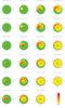 |
Fig. E.1 C+ fractionation structure as function of relative clump radius r/Rtot for different values of n and M. Each sector corresponds to a different χ value. The FR is color coded, ratios within ± 10% of the ER are shown in green. Blue and violet denotes FR < ER, yellow and red denotes FR > ER. |
Here we show fractionation plots of selected species over a large portion of our model parameter space. We left out models with M = 103 M⊙ because they show very similar results as models with M = 102 M⊙. The fractionation plots are also available for download: http://www.astro.uni-koeln.de/kosma-tau.
The comparison results and code descriptions are available at http://www.astro.uni-koeln.de/pdr-comparison
We recently updated KOSMA-τ to self-consistently account for various dust compositions and dust size distributions including wavelength-dependent continuum radiative transfer, dust temperature computation and photo-electric heating. For details see Röllig et al. (2013). However, the update was not fully available when we started this study, so we do not fully use the updated code capabilities here.
The isotopized chemical data set as well as the isotopization routine are available online: http://www.astro.uni-koeln.de/kosma-tau
The most recent set of shielding rates is predicted by Visser et al. (2009). In this work we still used the rates from van Dishoeck & Black (1988). Under most parameter conditions the model results differ only marginally (~10%) when switching to the new shielding rates.
12CO could also shield its less abundant relatives, if their absorption lines are sufficiently close together. However, only very few of the efficiently dissociating lines overlap, too few for mutual shielding to be important (Warin et al. 1996).
Acknowledgments
We acknowledge the use of OSU (http://www.physics.ohio-state.edu/~eric/research.html), KIDA (KInetic Database for Astrochemistry (http://kida.obs.u-bordeaux1.fr), and UDFA (http://www.udfa.net/) chemical reaction data bases. This work was supported by the German Deutsche Forschungsgemeinschaft, DFG project number Os 177/1–1 as well as within the Collaborative Research Council 956, sub-project C1, funded by the DFG.
References
- Agúndez, M., Goicoechea, J. R., Cernicharo, J., Faure, A., & Roueff, E. 2010, ApJ, 713, 662 [NASA ADS] [CrossRef] [Google Scholar]
- Asplund, M., Grevesse, N., & Sauval, A. J. 2005, in Cosmic Abundances as Records of Stellar Evolution and Nucleosynthesis, eds. T. G. Barnes, III, & F. N. Bash, ASP Conf. Ser., 336, 25 [Google Scholar]
- Bakes, E. L. O., & Tielens, A. G. G. M. 1994, ApJ, 427, 822 [NASA ADS] [CrossRef] [Google Scholar]
- Boreiko, R. T., & Betz, A. L. 1996, ApJ, 467, L113 [NASA ADS] [CrossRef] [Google Scholar]
- Casassus, S., Stahl, O., & Wilson, T. L. 2005, A&A, 441, 181 [NASA ADS] [CrossRef] [EDP Sciences] [Google Scholar]
- Centurion, M., Cassola, C., & Vladilo, G. 1995, A&A, 302, 243 [NASA ADS] [Google Scholar]
- Cubick, M., Stutzki, J., Ossenkopf, V., Kramer, C., & Röllig, M. 2008, A&A, 488, 623 [NASA ADS] [CrossRef] [EDP Sciences] [Google Scholar]
- Draine, B. T. 1978, ApJS, 36, 595 [NASA ADS] [CrossRef] [Google Scholar]
- Gerin, M., de Luca, M., Goicoechea, J. R., et al. 2010, A&A, 521, L16 [Google Scholar]
- Goicoechea, J. R., Pety, J., Gerin, M., et al. 2006, A&A, 456, 565 [NASA ADS] [CrossRef] [EDP Sciences] [Google Scholar]
- Hollenbach, D. J., & Tielens, A. G. G. M. 1999, Rev. Mod. Phys., 71, 173 [Google Scholar]
- Keene, J., Schilke, P., Kooi, J., et al. 1998, ApJ, 494, L107 [NASA ADS] [CrossRef] [Google Scholar]
- Kramer, C., Cubick, M., Röllig, M., et al. 2008, A&A, 477, 547 [NASA ADS] [CrossRef] [EDP Sciences] [Google Scholar]
- Kramer, C., Jakob, H., Mookerjea, B., et al. 2004, A&A, 424, 887 [NASA ADS] [CrossRef] [EDP Sciences] [Google Scholar]
- Langer, W. D., Graedel, T. E., Frerking, M. A., & Armentrout, P. B. 1984, ApJ, 277, 581 [NASA ADS] [CrossRef] [Google Scholar]
- Langer, W. D., & Penzias, A. A. 1990, ApJ, 357, 477 [NASA ADS] [CrossRef] [Google Scholar]
- Langer, W. D., & Penzias, A. A. 1993, ApJ, 408, 539 [NASA ADS] [CrossRef] [Google Scholar]
- Le Bourlot, J., Pineau Des Forets, G., Roueff, E., & Flower, D. R. 1993, A&A, 267, 233 [NASA ADS] [Google Scholar]
- Le Bourlot, J., Le Petit, F., Pinto, C., Roueff, E., & Roy, F. 2012, A&A, 541, A76 [NASA ADS] [CrossRef] [EDP Sciences] [Google Scholar]
- Le Petit, F., Nehmé, C., Le Bourlot, J., & Roueff, E. 2006, ApJS, 164, 506 [NASA ADS] [CrossRef] [EDP Sciences] [Google Scholar]
- Lee, H.-H., Herbst, E., Pineau des Forets, G., Roueff, E., & LeBourlot, J. 1996, A&A, 311, 690 [NASA ADS] [Google Scholar]
- Liszt, H. S. 2007, A&A, 476, 291 [NASA ADS] [CrossRef] [EDP Sciences] [Google Scholar]
- Magnani, L., Lugo, S., & Dame, T. M. 2005, AJ, 130, 2725 [NASA ADS] [CrossRef] [Google Scholar]
- Magnani, L., Zelenik, S., Dame, T. M., & Engebreth, B. 2006, ApJ, 636, 267 [NASA ADS] [CrossRef] [Google Scholar]
- Mattila, K. 1986, A&A, 160, 157 [NASA ADS] [Google Scholar]
- Mookerjea, B., Kramer, C., Röllig, M., & Masur, M. 2006, A&A, 456, 235 [NASA ADS] [CrossRef] [EDP Sciences] [Google Scholar]
- Mookerjea, B., Ossenkopf, V., Ricken, O., et al. 2012, A&A, 542, L17 [NASA ADS] [CrossRef] [EDP Sciences] [Google Scholar]
- Ossenkopf, V., Röllig, M., Neufeld, D., et al. 2013, A&A, 550, A57 (Paper II) [NASA ADS] [CrossRef] [EDP Sciences] [Google Scholar]
- Qin, S.-L., Schilke, P., Comito, C., et al. 2010, A&A, 521, L14 [NASA ADS] [CrossRef] [EDP Sciences] [Google Scholar]
- Rachford, B. L., Snow, T. P., Tumlinson, J., et al. 2002, ApJ, 577, 221 [NASA ADS] [CrossRef] [Google Scholar]
- Ritchey, A. M., Federman, S. R., & Lambert, D. L. 2011, ApJ, 728, 36 [NASA ADS] [CrossRef] [Google Scholar]
- Röllig, M. 2011, A&A, 530, A9 [NASA ADS] [CrossRef] [EDP Sciences] [Google Scholar]
- Röllig, M., Ossenkopf, V., Jeyakumar, S., Stutzki, J., & Sternberg, A. 2006, A&A, 451, 917 [NASA ADS] [CrossRef] [EDP Sciences] [Google Scholar]
- Röllig, M., Abel, N. P., Bell, T., et al. 2007, A&A, 467, 187 [NASA ADS] [CrossRef] [EDP Sciences] [Google Scholar]
- Röllig, M., Kramer, C., Rajbahak, C., et al. 2011, A&A, 525, A8 [Google Scholar]
- Röllig, M., Szczerba, R., Ossenkopf, V., & Glück, C. 2013, A&A, 549, A85 [NASA ADS] [CrossRef] [EDP Sciences] [Google Scholar]
- Sheffer, Y., Rogers, M., Federman, S. R., Lambert, D. L., & Gredel, R. 2007, ApJ, 667, 1002 [NASA ADS] [CrossRef] [Google Scholar]
- Sheffer, Y., Rogers, M., Federman, S. R., et al. 2008, ApJ, 687, 1075 [NASA ADS] [CrossRef] [Google Scholar]
- Smith, D., & Adams, N. G. 1980, ApJ, 242, 424 [NASA ADS] [CrossRef] [Google Scholar]
- Sonnentrucker, P., Welty, D. E., Thorburn, J. A., & York, D. G. 2007, ApJS, 168, 58 [NASA ADS] [CrossRef] [Google Scholar]
- Stacey, G. J., Townes, C. H., Geis, N., et al. 1991, ApJ, 382, L37 [NASA ADS] [CrossRef] [Google Scholar]
- Sternberg, A., & Dalgarno, A. 1989, ApJ, 338, 197 [NASA ADS] [CrossRef] [Google Scholar]
- Sternberg, A., & Dalgarno, A. 1995, ApJS, 99, 565 [NASA ADS] [CrossRef] [Google Scholar]
- Störzer, H., Stutzki, J., & Sternberg, A. 1996, A&A, 310, 592 [NASA ADS] [Google Scholar]
- Suutarinen, A., Geppert, W. D., Harju, J., et al. 2011, A&A, 531, A121 [NASA ADS] [CrossRef] [EDP Sciences] [Google Scholar]
- van Dishoeck, E. F., & Black, J. H. 1988, ApJ, 334, 771 [NASA ADS] [CrossRef] [Google Scholar]
- van Dishoeck, E. F., Jonkheid, B., & van Hemert, M. C. 2006, Faraday Discussions, 133, 231 [NASA ADS] [CrossRef] [PubMed] [Google Scholar]
- van Hemert, M. C., & van Dishoeck, E. F. 2008, Chem. Phys., 343, 292 [NASA ADS] [CrossRef] [Google Scholar]
- Visser, R., van Dishoeck, E. F., & Black, J. H. 2009, A&A, 503, 323 [NASA ADS] [CrossRef] [EDP Sciences] [Google Scholar]
- Wakelam, V., & Herbst, E. 2008, ApJ, 680, 371 [NASA ADS] [CrossRef] [Google Scholar]
- Wakelam, V., Herbst, E., Loison, J.-C., et al. 2012, ApJS, 199, 21 [NASA ADS] [CrossRef] [Google Scholar]
- Warin, S., Benayoun, J. J., & Viala, Y. P. 1996, A&A, 308, 535 [NASA ADS] [Google Scholar]
- Watson, W. D., Anicich, V. G., & Huntress, Jr., W. T. 1976, ApJ, 205, L165 [NASA ADS] [CrossRef] [Google Scholar]
- Weingartner, J. C., & Draine, B. T. 2001, ApJ, 548, 296 [NASA ADS] [CrossRef] [Google Scholar]
- Woodall, J., Agúndez, M., Markwick-Kemper, A. J., & Millar, T. J. 2007, A&A, 466, 1197 [NASA ADS] [CrossRef] [EDP Sciences] [Google Scholar]
- Woods, P. M., & Willacy, K. 2009, ApJ, 693, 1360 [NASA ADS] [CrossRef] [Google Scholar]
- Woon, D. E., & Herbst, E. 2009, ApJS, 185, 273 [NASA ADS] [CrossRef] [Google Scholar]
- Wouterloot, J. G. A., & Brand, J. 1996, A&AS, 119, 439 [NASA ADS] [CrossRef] [EDP Sciences] [Google Scholar]
All Tables
All Figures
|
Fig. 1 Radial density profile of a model clump. The dashed lines show the density profile along various lines of sight (for different impact parameters p). |
| In the text | |
|
Fig. 2 CO shielding factors12 of a model clump with the following model parameters: n0 = 105 cm-3, M = 100 M⊙, χ = 10 (CO: solid line, 13CO: dashed line). |
| In the text | |
|
Fig. 3 Chemical structure of a model clump with the following model parameters: n0 = 105 cm-3, M = 100 M⊙, χ = 10. (main isotopologue: solid line, 13C isotopologue multiplied by ER = 67: dashed line). |
| In the text | |
|
Fig. 4 Fractionation structure of the same model clump as shown in Fig. 3 (solid lines: fractionation ratios n(X)/n(13X), dashed line: kinetic gas temperature (right axis). |
| In the text | |
|
Fig. 5 Reaction rates for the same model clump as shown in Fig. 3 (photo-dissociation of CO: black, solid; 13CO: black, dashed; back and forth reaction rates in reaction (C 1): red). |
| In the text | |
|
Fig. 6 Fractionation structure as function of relative clump radius r/Rtot for n = 103 cm-3 and M = 1 M⊙. Each sector corresponds to a different χ value. The FR is color coded, ratios within ± 10% of the ER are shown in green. Left panel: FR of C+, the color scale goes from 0 to 2000. Right panel: FR of CO, the color scale goes from 0 to 100. |
| In the text | |
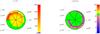 |
Fig. 7 Same as Fig. 6 for n = 105 cm-3 and M = 1 M⊙. |
| In the text | |
|
Fig. 8 Comparison of the AV,12CT and AV,13CT, i.e. the AV, where n(C + ) = n(CO) and |
| In the text | |
|
Fig. 9 Scatter plot of the mean column density fractionation ratio vs. the mean column density of the main isotopologue of CO/13CO of the whole parameter space. The model parameters n, M, and χ, are coded as size, shape, and color of the respective symbols. The red line denotes the model elemental abundance [12C]/[13C] = 67. |
| In the text | |
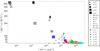 |
Fig. 10 Same as Fig. 9 for C+. |
| In the text | |
|
Fig. 11 Fractionation structure of the very dense model clump. The model parameters are n = 107 cm-3,M = 0.01 M⊙,χ = 105. (Main isotopologue: solid lines, 13C isotopologue multiplied by ER = 67: dashed lines.) |
| In the text | |
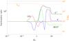 |
Fig. 12 Fractionation structure of the same model clump as shown in Fig. 11. |
| In the text | |
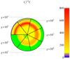 |
Fig. 13 Same as Fig. 6 for C for n = 105 cm-3 and M = 1 M⊙. |
| In the text | |
|
Fig. 14 Chemical network of the dominant formation and destruction channels for: left panel: CH+, CH |
| In the text | |
|
Fig. 15 Fractionation structure of light hydrocarbons for n0 = 105 cm-3, M = 100 M⊙, χ = 10 (green: FR(C), red ER). |
| In the text | |
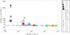 |
Fig. 16 Same as Fig. 9 for CH+. |
| In the text | |
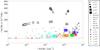 |
Fig. 17 Same as Fig. 9 for CH. |
| In the text | |
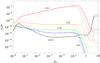 |
Fig. 18 Same as Fig. 3 for species HCO+, CH, CH+, CH |
| In the text | |
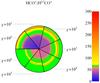 |
Fig. 19 Same as Fig. 6 for HCO+ for n = 105 cm-3 and M = 1 M⊙. |
| In the text | |
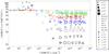 |
Fig. 20 Same as Fig. 9 for HCO+. |
| In the text | |
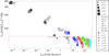 |
Fig. 21 Same as Fig. 9 for the intensity ratio Tmb( [CII] )/Tmb( [13CII] ) vs. Tmb( [CII] ). |
| In the text | |
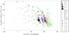 |
Fig. 22 Same as Fig. 21 for Tmb(CO(1−0))/Tmb(13CO(1−0)) vs. Tmb(CO(1−0)). |
| In the text | |
|
Fig. 23 Emission line ratio Tmb(CO(J → J − 1))/Tmb(13CO(J → J − 1)) vs. J for all models with M = 10 M⊙. Models with line intensities < 0.01 K km s-1 have been omitted. |
| In the text | |
|
Fig. 24 Column density fractionation ratios plotted against the emission line ratio Tmb( [CII] )/Tmb(H13CO + (1 − 0)) for all models from our parameter space (blue: ER, red: ER ± 10%, dashed: ER ± 20%). The symbols follow the coding from Fig. 9. The gray areas denote the regime below a sensitivity limit of Tmb < 0.01 K km s-1. Left panel: N(CO)/N(13CO), middle panel: N(C)/N(13C), right panel: |
| In the text | |
|
Fig. 25 Column density fractionation ratios plotted against emission line ratios for all models from our parameter space. (blue: ER, red: ER ± 10 %, dashed: ER ± 20%). Models with line intensities < 0.01 K km s-1 have been omitted. The symbols follow the coding from Fig. 9. Left panel: N(CO)/N(13CO) vs. Tmb(13CO(2 − 1))/Tmb( [CI] 610 μm), middle panel: N(C)/N(13C) vs. Tmb( [CII] )/Tmb(H13CO + (1 − 0)), right panel: |
| In the text | |
|
Fig. C.1 Chemical structure of a model clump with the following model parameters: n0 = 105 cm-3, M = 100 M⊙, χ = 10 (UDfA06 (solid), OSU (dashed), KIDA (dotted). The gray shaded area shows the gas temperature spanned by the three models calculations. |
| In the text | |
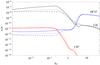 |
Fig. C.2 Same as Fig. C.1 for HCO+, CH, and CH+. |
| In the text | |
|
Fig. C.3 Mean CH column density versus H2 column density (color/shape coding same as Fig. 9). Observational results are plotted as colored points (red: Sheffer et al. 2008; green: Rachford et al. 2002; olive: Magnani et al. 2005; black: Qin et al. 2010; brown: Magnani et al. 2006; orange Gerin et al. 2010; blue Suutarinen et al. 2011). The two lines are the CH − H2 relations from Mattila (1986) (red) and Qin et al. (2010) (black). |
| In the text | |
|
Fig. E.1 C+ fractionation structure as function of relative clump radius r/Rtot for different values of n and M. Each sector corresponds to a different χ value. The FR is color coded, ratios within ± 10% of the ER are shown in green. Blue and violet denotes FR < ER, yellow and red denotes FR > ER. |
| In the text | |
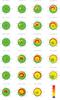 |
Fig. E.2 Same as Fig. E.1 for C. |
| In the text | |
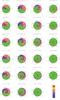 |
Fig. E.3 Same as Fig. E.1 for CO. |
| In the text | |
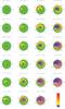 |
Fig. E.4 Same as Fig. E.1 for HCO+. |
| In the text | |
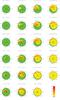 |
Fig. E.5 Same as Fig. E.1 for CH. |
| In the text | |
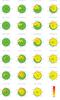 |
Fig. E.6 Same as Fig. E.1 for CH+. |
| In the text | |
Current usage metrics show cumulative count of Article Views (full-text article views including HTML views, PDF and ePub downloads, according to the available data) and Abstracts Views on Vision4Press platform.
Data correspond to usage on the plateform after 2015. The current usage metrics is available 48-96 hours after online publication and is updated daily on week days.
Initial download of the metrics may take a while.