| Issue |
A&A
Volume 550, February 2013
|
|
|---|---|---|
| Article Number | A103 | |
| Number of page(s) | 13 | |
| Section | Stellar atmospheres | |
| DOI | https://doi.org/10.1051/0004-6361/201220064 | |
| Published online | 04 February 2013 | |
Convective line shifts for the Gaia RVS from the CIFIST 3D model atmosphere grid⋆,⋆⋆
1
Instituto de Astrofísica de Canarias, 38205
La Laguna, Tenerife,
Spain
2
Departamento de Astrofísica, Universidad de La
Laguna, 38206,
La Laguna, Tenerife,
Spain
e-mail: This email address is being protected from spambots. You need JavaScript enabled to view it.
3
Texas Advanced Computing Center, University of
Texas, Austin,
TX
78759,
USA
e-mail: This email address is being protected from spambots. You need JavaScript enabled to view it.
4
Zentrum für Astronomie der Universität Heidelberg,
Landessternwarte, Königstuhl 12,
69117
Heidelberg,
Germany
e-mail: This email address is being protected from spambots. You need JavaScript enabled to view it.
; This email address is being protected from spambots. You need JavaScript enabled to view it.
5
Centre de Recherche Astrophysique de Lyon, UMR 5574, CNRS,
Université de Lyon, École Normale
Supérieure de Lyon, 46 allée d’Italie, 69364
Lyon Cedex 07,
France
e-mail: This email address is being protected from spambots. You need JavaScript enabled to view it.
Received: 20 July 2012
Accepted: 26 November 2012
Abstract
Context. To derive space velocities of stars along the line of sight from wavelength shifts in stellar spectra requires accounting for a number of second-order effects. For most stars, gravitational redshifts, convective blueshifts, and transverse stellar motion are the dominant contributors.
Aims. We provide theoretical corrections for the net velocity shifts due to convection expected for the measurements from the Gaia Radial Velocity Spectrometer (RVS).
Methods. We used a set of three-dimensional time-dependent simulations of stellar surface convection computed with CO5BOLD to calculate spectra of late-type stars in the Gaia RVS range and to infer the net velocity offset that convective motions will induce in radial velocities derived by cross-correlation.
Results. The net velocity shifts derived by cross-correlation depend both on the wavelength range and spectral resolution of the observations. Convective shifts for Gaia RVS observations are less than 0.1 km s-1 for late-K-type stars, and they increase with stellar mass, reaching about 0.3 km s-1 or more for early F-type dwarfs. This tendency is the result of an increase with effective temperature in both temperature and velocity fluctuations in the line-forming region. Our simulations also indicate that the net RVS convective shifts can be positive (i.e. redshifts) in some cases. Overall, the blueshifts weaken slightly with increasing surface gravity, and are enhanced at low metallicity. Gravitational redshifts amount to 0.7 km s-1 and dominate convective blueshifts for dwarfs, but become much weaker for giants.
Key words: stars: atmospheres / line: formation / convection / techniques: radial velocities / stars: solar-type / stars: late-type
Appendix A is available in electronic form at http://www.aanda.org
Model spectra from the 1D and 3D calculations are only available in electronic form at the CDS via anonymous ftp to cdsarc.u-strasbg.fr130.79.128.5 or via http://cdsarc.u-strasbg.fr/viz-bin/qcat?J/A+A/550/A103
© ESO, 2013
1. Introduction
Stellar atmospheres are not in hydrostatic equilibrium. Convection, magnetic fields, rotation, oscillations, and other phenomena induce time and spatially changing structure on the surfaces of stars. In the case of late-type stars, surface convection is responsible for the granulation pattern directly observed in high-resolution pictures of the Sun.
Granulation broadens absorption line profiles in observed solar spectra, making them asymmetric and introducing a net blueshift in their central wavelengths. Even though the typical granular velocities reach several kilometers per second, the net blueshift observed in spatially-averaged spectra of solar photospheric lines rarely exceeds 1 km s-1. In solar-type stars, the photosphere is usually located above the convectively unstable zone and the velocity field weakens with height. This causes the net convective shift to be strongest for lines formed in deep layers, progressively weakening and then disappearing for lines formed higher up in the photosphere (Allende Prieto & García López 1998; Pierce & Lopresto 2000; Ramírez et al. 2008; Gray 2009).
Stellar spectra are often used to measure the velocities of stars projected along the line of sight. The interpretation of the measured line wavelength shifts in terms of Doppler shifts purely associated with bulk stellar motion results in biased radial velocities owing to the presence of photospheric velocity fields. Furthermore, motions in stellar atmospheres are not the only mechanism that can bias radial velocity measurements, and a number of other effects, most notably gravitational redshifts (e.g., Pasquini et al. 2011), frustrate the direct derivation of the line-of-sight component of the velocity of a star’s center of mass from the spectrum. Correcting for all these effects involves knowledge that is usually uncertain and, in most cases, model dependent, and therefore the IAU recommends using the term “radial-velocity measure” to refer to the velocity naively inferred from the spectral shifts under classical Newtonian mechanics, ignoring the corrections mentioned earlier (Lindegren & Dravins 2003).
The ESA mission Gaia is scheduled for launch in late 2013 with the purpose of measuring proper motions, parallaxes, and spectrophotometry for some 109 stars down to V ~ 20 mag, and spectra for about 108 stars down to V ~ 17 mag (de Bruijne et al. 2009; Lindegren 2010). The typical uncertainty of the radial-velocity measures provided by Radial Velocity Spectrometer (RVS) onboard Gaia (Katz et al. 2004; Wilkinson et al. 2005) will typically be in the range 1−20 km s-1, but taking the average for large groups of stars will largely reduce the uncertainties, and the systematic errors discussed above can become dominant if neglected. More important, the RVS does not have any onboard calibration source to rely on for wavelength calibration, and systematic effects need to be considered, since wavelength calibration is based on a subset of the very same stellar spectra obtained by RVS (Katz et al. 2011).
As nature favors the formation of stars with low masses, we focus our attention on late-type stars, for which systematic errors affecting the translation from spectral shifts to bulk velocities are mainly gravitational redshifts, convective shifts, and the effect of the transversal motion on the relativistic Doppler effect. With the parallaxes measured by Gaia, through the comparison of colors and absolute brightness with stellar evolution theory, it will be possible to estimate masses and radii to calculate gravitational redshifts to better than 10% (Allende Prieto & Lambert 1999), or some 50 m s-1 for a solar-like star. Accurate proper motions and parallaxes will also provide accurate transversal motions. With the exception of the Sun, it is very difficult to disentangle convective shifts from the bulk stellar motion, and therefore it becomes necessary to rely on models.
We have shown that modern three-dimensional hydrodynamical models of the solar surface can accurately predict the convective shifts of individual weak and moderate-strength photospheric iron lines to within 70 m s-1 (Allende Prieto et al. 2009). The same models, however, predict net redshifts, which are not observed, for very strong iron lines (Allende Prieto et al. 2009; see also Asplund et al. 2000). Convective shifts need to be evaluated for specific spectral windows used in the derivation of radial velocities, ensuring that models are appropriate for those windows.
In this paper, we focus our attention on the observations to be obtained by the Gaia RVS and predict convective wavelength shifts for stars of spectral types M through A (3500 < Teff < 7000 K) from a collection of hydrodynamical simulations presented by Ludwig et al. (2009). As such corrections are specifically derived for the Gaia RVS, and in particular for radial velocity measures derived by cross-correlation of RVS spectra with template spectra calculated from classical (hydrostatic) model atmospheres, we will refer to them, indistinctively, as net convective shifts or effective convective shifts for RVS spectra.
Section 2 describes the hydrodynamical simulations. Section 3 is devoted to the spectral synthesis calculations, and Sect. 4 describes the results. In Sect. 5 we comment briefly on the size of the gravitational shifts expected for the same stars previously modeled, and Sect. 6 presents a summary of our findings.
2. Model atmospheres
Simulations of stellar surface convection for 83 combinations of surface gravity, entropy flux at the bottom of the atmosphere, and chemical composition were computed using the code CO5BOLD (Freytag et al. 2002; Wedemeyer et al. 2004; Freytag et al. 2012). The code solves the equations of hydrodynamics in a Cartesian grid with periodic horizontal boundary conditions and accounting for the effect of the radiation field on the energy balance.
The models typically have a resolution of 140 × 140 × 150 (X-Y-Z) grid points, corresponding to physical sizes significantly larger than the typical size of granules, and range from a few Mm for dwarfs to thousands of Mm for giant stars. The radiation field applying a multi-group technique (Nordlund 1982) using 5 groups for models of solar and 6 groups for models of subsolar metallicity. The number of groups was chosen by trial-and-error to ensure an acceptable representation of the radiative cooling or heating effects. This was done primarily by looking at solar-like stars. It turned out, however, that also giants, as well as hotter and cooler dwarfs could be treated in the same way obtaining similar accuracies. It was found that at subsolar metallicities the treatment of the radiative transfer in the continuum is more critical so that an extra group was introduced.
We believe that the typically employed five or six groups are sufficient for obtaining accurate line shifts, but this is difficult to demonstrate in general since only for few cases are models with more groups available. However, the line shifts hinge very much on the velocity field which is driven in deeper layers, where the wavelength dependence of the radiative transfer becomes of secondary importance. In the few models employing 12 groups that are available, changes in the level of the temperature fluctuations are not large. We think that rather spatial resolution and sampling of the time series dominate the uncertainties in the line shifts.
The equation of state takes into account H and He ionization and H2 formation, while the opacities are calculated with the Uppsala package (Gustafsson et al. 2008). The physical size of the computational box is the same for models with the same surface temperature and gravity. The upper boundary of the models is open, and extended beyond a Rosseland optical depth of 10-6, while the lower boundary is well into optically thick, convectively unstable layers. Each simulation was run until fully relaxed. Chemical abundances are from Grevesse & Sauval (1998), with the exception of CNO, which are updated following Asplund (2005). More details are provided by Ludwig et al. (2009).
For each simulation, a set of uncorrelated snapshots was selected for spectral synthesis. The number of snapshots and the total time span of the simulations varied from star to star, according to the granular turn-over time scale for each model. The snapshots were hand chosen in order to be representative of the whole simulated time series, avoiding statistical anomalies. We found from tests that about 20 uncorrelated snapshots are enough to represent a model, but in some cases a smaller number was adequate.
In order to determine the net convective shift predicted for each 3D model, we calculated a 1D model atmosphere with the same effective temperature, surface gravity and metallicity. The effective temperature for each simulation was determined from the temporally and spatially averaged emergent bolometric flux. The 1D models were calculated with the LHD package (Caffau & Ludwig 2007), and share the basic ingredients (most importantly the opacities and equation of state) with the 3D simulations. A second comparison set of 1D models was derived by linear interpolation of the ODFNEW model grid by Castelli & Kurucz1 (2004), based on the solar abundances of Grevesse & Sauval (1998).
3. Spectral synthesis
3.1. 3D spectral synthesis
We computed synthetic spectra covering the Gaia RVS wavelength range (847−874 nm) with wavelength steps equivalent to ≤0.1 km s-1 (or a resolving power R ≡ λ/δλ ~ 106). The calculations were carried out with the 3D synthesis code ASSϵT (Koesterke 2009; Koesterke et al. 2008). The reference solar abundances are from Asplund et al. (2005), and while temperature, density and velocity fields were taken from the model atmospheres, the electron density was recalculated with an equation of state including the first 99 elements in the periodic table and 338 molecules (Tsuji 1973, with partition functions from Irwin 1981).
The number of snapshots used varied between 8 and 21, but in the vast majority of cases was about 20, and the total time covered ranged between 0.6 and 19 500 h, spanning at least 10 times the typical lifetimes of convective cells. The number of pixels considered for each snapshot was reduced by taking one out of three points in the X- and Y-directions, and at least the uppermost 90 vertical points. These choices are based on previous experience and limited testing with the set of models used in this paper. These tests indicate that dropping spatial points would lead only to differences at the level of about 0.2% for a typical strong Fe I line. For the continuum and weak lines the differences tend to be much smaller than that.
The adopted solar abundances are very similar to those used in the 3D simulations. The small existing inconsistencies are expected to have a negligible impact in the predicted convective shifts. Continuous absorption from H and H− is included. Line absorption is included in detail from the atomic and molecular files compiled by Kurucz. Opacities are precomputed in a temperature-density grid bracketing all the snapshots with steps of 250 K and 0.25 dex, and subsequently derived for the grid points using cubic Bézier interpolation.
For each individual snapshot a spectrum is derived in 2 steps. First a background radiation field is calculated. This is used for the scattering term in the subsequent spectrum synthesis. Note that actually 2 spectra are calculated for each snapshot. The second one, which is derived from opacity data without spectral lines, is used for continuum normalization.
The radiative transfer calculations account for atomic hydrogen Rayleigh and electron scattering. The mean background radiation field is calculated from 24 angles (8 azimuthal with linear weights, and 3 zenith per half-sphere with Gaussian weights) using a short characteristics scheme, while the emergent flux is integrated for 21 angles (vertical ray plus 3 zenithal rays and 8 azimuthal angles again with linear weights, except that only 4 zenithal angles are considered for the shallowest rays). The abscissae and weights for each case can be found in Abramowitz & Stegun (1972). This setup evenly covers a sphere with 8 angles for the azimuth (0−360 deg) and 3−4 angles for the inclination (0−180 deg). The integration along a ray was performed from the top layer down to optical depths of at least 20. The final emergent flux is an average of the flux for all the snapshots considered for each simulation.
Rotation was not accounted for in this step. It is well-known that rotation affects the observed line asymmetries (Gray 1986), but low rotational velocities should only have a modest effect on the net shifts derived by cross-correlation for the entire Gaia RVS spectral window. In part, this is related to the spectral resolution of the RVS instrument, corresponding to 26 km s-1 (de Bruijne 2012).
The calculations were performed on the Longhorn cluster at the Texas Advanced Computing Center (TACC). The intensities for about 150 million frequencies were derived across all snapshots. The total computational effort is roughly equivalent to 3 months on a modern workstation with 4 cores.
Figure 1 illustrates the spectra in our 1D and 3D grids that are closest to the atmospheric parameters for Arcturus and the Sun. This comparison is done after smoothing the data to a FWHM resolving power of R = 11 500 as appropriate for the RVS; we adopted a microturbulent velocity of 1.5 km s-1 for the 1D calculations. The agreement between models and observations is significantly better in the solar case (observed spectrum from Kurucz et al. 1984) than for Arcturus (Hinkle et al. 2000). Overall, predicted absorption features are slightly stronger in 1D than in 3D. The agreement is reasonable, considering that the models are not tailored to these stars. Arcturus has an Teff ~ 4300 K, log g ≃ 1.7 (with g in cm s-2) and a metallicity about [Fe/H] ≃ −0.5 (see, e.g., Ramírez & Allende Prieto 2011), and the Sun has an Teff = 5777 K, log g ≃ 4.437 and, by definition, [Fe/H] = 0 (see, e.g. Stix 2004). The model compared here with Arcturus (d3t40g15mm10n01) has an Teff of 4040 K, log g = 1.5 and a metallicity of [Fe/H] = −1.0, and that compared with the Sun (d3t59g45mm00n01) has an Teff of 5865 K, log g = 4.5 and solar metallicity.
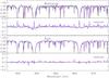 |
Fig. 1 Observed (black line) and synthetic (1D in red, 3D in blue) spectra for Arcturus and the Sun – all data smoothed with a Gaussian kernel to have a resolving power of about 11 500 as appropriate for the Gaia RVS. Both the normalized spectra and the residuals are shown for each star. A microturbulence of 1.5 km s-1 was adopted for the 1D models, which were calculated with the LHD package. |
3.2. 1D spectral synthesis
The 1D counterpart radiative transfer calculations were performed with the 1D version of ASSϵT, and therefore the results can be directly compared between the 1D and 3D models. In particular, chemical compositions, opacities, and radiative transfer calculation for the emergent intensities are shared by the 1D and 3D branches. The only differences between the 1D and 3D calculations are that the opacities are calculated exactly for the grid points in 1D (every depth in the model atmospheres), while they are interpolated in 3D (from a precomputed grid in temperature and density, as described in Sect. 3.1), and the radiative transfer solver for the calculation of the mean intensities in the grid, which is based on Feautrier’s method (Feautrier 1964) in 1D and an integral method in 3D. Our tests nonetheless indicate that these differences have a negligible effect on the continuum-normalized fluxes. The difference between the Feautrier and the direct method in 1D is about 10-5. The effect of the interpolation of the opacities in 3D is estimated to be on the order of 10-4. The different choices for the opacity calculation and the radiation transfer method are made to accommodate the very expensive calculations in 3D, which are not feasible without interpolating the opacities and benefit from the faster 1st order method for the integration of the intensities.
4. Effective convective shifts for the Gaia RVS
We divided the spectra by the pseudo continua, estimated by iteratively fitting a low order polynomial to the upper envelope of each spectrum. We then calculated the net offset between the 3D and 1D spectra to derive the overall convective shift predicted by the hydrodynamical simulations by cross-correlation.
The cross-correlation of two arrays (o spectra) T and S of equal and even number of elements N is defined as a new array C with 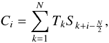 (1)where i runs from 1 to N. If the spectrum T is identical to S, but shifted by an an integer number of pixels p, the maximum value in the array C will correspond to its element
  . Cross-correlation can be similarly used to measure shifts that correspond to non-integer numbers. In this case, finding the location of the maximum value of the cross-correlation function can be performed with a vast choice of algorithms.
We calculated the cross-correlation of 1D and 3D model spectra using the software by Allende Prieto (2007), which allows fitting the peak of the cross-correlation function with a parabola, a cubic polynomial, or a Gaussian. Based on tests adding noise to simulated spectra, we chose to use parabolic fittings to the central 3 points around the maximum of the cross-correlation function.
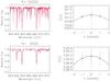 |
Fig. 2 Spectra for a single snapshot of model d3t59g45mm00n01 (black) and its 1D counterpart (black), with near solar atmospheric parameters, are shown in the left-hand panels for two different values of the resolving power (R). The right-hand panels illustrate how the corresponding shifts (1D relative to 3D) are obtained by fitting the peak of the cross-correlation function with a parabola. |
 |
Fig. 3 Derived convective shift for model d3t59g45mm00n01, with near solar atmospheric parameters, as a function of the resolving power. These shifts are obtained by cross-correlation using the Gaia RVS spectral window, and fitting the peak of the cross-correlation function with a parabola. The dashed vertical line marks the RVS resolving power. |
The net convective shift derived by cross-correlation not only depends on the chosen spectral range, but also on the resolving power of the spectrograph. A degraded resolution will introduce, in addition to random noise, a systematic error in the derived velocity shifts. This is illustrated in Fig. 2 for a single 3D snapshot and its 1D counterpart at two different values of the resolving power: resolution does change the apparent convective shift. Figure 3 shows the derived shifts (1D relative to 3D) for model d3t59g45mm00n01 (see Table 1 for reference), which was compared with the solar spectrum in Fig. 1, as a function of the resolving power. At the resolving power of the Gaia RVS (R = 11 500), the inferred convective blueshift is about 0.1 km s-1, while that measured when the spectral lines are fully resolved (R > 200 000) approaches 0.24 km s-1. Our results for the simulations are included in Table 1. All the values presented in the table, and discussed below correspond to the RVS resolution.
In addition to calculating the net convective shifts for the average spectra from the selected snapshots for each simulation, we also calculated the shifts for each snapshot and averaged them out. These correspond to the “mean” shifts in Table 1. The variance (σ2) among snapshots was used to estimate the intrinsic uncertainties as  , with n the number of snapshots considered, and these are also included in the table. We believe that the uncertainties calculated in this way are conservative since the subsample of snapshots selected for spectral synthesis is chosen to represent the properties of the complete run (e.g., in effective temperature and mean velocities). Moreover, the separation in time among the snapshots is large enough that they can be considered as independent despite being selected from one time series. The agreement between the shifts of the average spectra and the average shifts from individual snapshots is excellent, with an average of 0.0004 km s-1 and a standard deviation of 0.001 km s-1.
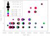 |
Fig. 4 Effective convective shifts predicted by the 3D hydrodynamical models for Gaia RVS observations. |
Figure 4 shows the convective shifts for all models. Note that there are models for four different metallicities, color−coded, and that the resulting effective temperatures of the simulations are not always exactly the same for any combination of surface gravity and metallicity, as this is not an input parameter – the entropy of the material entering the simulations box through the open bottom boundary is a chosen input instead.
The changes of the net convective shifts with the atmospheric parameters are perhaps most obvious in Fig. 5. The net shifts show a mild correlation with the effective temperature of the models, in the sense that warmer stars tend to exhibit larger blueshifts. As found in previous studies (Dravins & Nordlund 1990a,b; Nordlund & Dravins 1990), the net energy flux traversing the atmosphere is the most important parameter. Surface gravity has a small effect on the convective shifts predicted by our simulations – overall the shifts intensify at lower gravities – and so has metallicity, with lower net blueshifts at higher metallicities. Figure 4 shows the results obtained when the LHD 1D models, which are fully consistent with the 3D simulations in terms of opacities and the equation of state, are used as reference. However, very similar results are found when Kurucz models are used as a reference (see below).
We adopted a micro-turbulence of 2.0 km s-1, and a macro-turbulence of 1.5 km s-1 for the reference 1D calculations, but our experiments indicate that these parameters would only lead to a modest impact on the spectral shifts determined by cross-correlation. For instance, completely neglecting macro-turbulence leads to a mean correction in the predicted convective blueshifts of just 0.01 (σ = 0.032) km s-1. Adopting a micro-turbulence of 1.5 km s-1 instead of 2.0 km s-1 will, on average, reduce the convective blueshifts by about 0.007 (σ = 0.011) km s-1. Finally, adopting Kurucz model atmospheres instead of LHD models as our 1D reference will, on average, enhance the blueshifts by about 0.01 (σ = 0.03) km s-1.
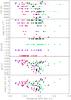 |
Fig. 5 Three uppermost panels: predicted convective shifts and atmospheric parameters of the 3D hydrodynamical models for Gaia RVS observations. Two lowermost panels: convective shifts versus relative horizontal temperature fluctuations and the rms of the vertical velocity at Rosseland optical depth τ = 2/3. In all panels data points are color coded by metallicity as in Fig. 4. |
The smallest (in absolute terms) convective shifts in the grid are for the coolest dwarfs of low metal content, and amount barely to <0.1 km s-1. The most vigorous net velocities are found for low metallicity F-type subgiants, practically the warmest stars considered in the grid, where they exceed 0.3 km s-1.
There are a few simulations (mostly with [Fe/H] = −1) for which redshifts are predicted. While perhaps not very evident in Fig. 5 the drop is clearly apparent in a global analytical fit of the convective shifts of the 3D simulations (see Appendix A). These redshifts are a clear prediction of the simulations. They are caused by strong redshifts of the cores of the Ca II triplet lines, but they dominate the overall cross-correlation signal. The cores get redshifted when the lines are strong and the flow exhibits a pronounced “reverse granulation” pattern. Still, the overall shift of the Ca II triplet line cores is a superposition of redshifted and blueshifted contributions and therefore it is difficult to predict a priori which ones are dominating.
We tried to interpret our findings in terms of the temperature and velocity fluctuations present in the 3D simulations. We averaged the temperature and vertical velocity component horizontally and temporally on surfaces of constant Rosseland optical depth. We took values at Rosseland depth τ = 2/3 as representative for the conditions prevailing in the line forming regions – at least for weak lines. These are shown in the two bottom panels of Fig. 5, where a mild correlation between temperature and velocity fluctuations is apparent.
Figure 6 shows how the temperature and velocity fluctuations depend on effective temperature, surface gravity and metallicity. Interestingly, we find that the velocity fluctuations depend on metallicity for Teff < 5000 K but they do not for warmer stars. Only close to the main-sequence a systematic dependence appears below 5000 K with higher metallicity implying greater fluctuations. For main-sequence stars, Teff = 5000 K also separates regions of different correlation between metallicity and temperature fluctuations. Above 5000 K, higher metallicity corresponds to lower temperature fluctuations but this is reversed below 5000 K. While Fig. 6 certainly motivates the increase in convective shifts towards higher effective temperatures and lower gravity, it cannot explain all trends of the convective shifts. What is indeed missing is information on the mutual correlation between temperature and velocity fluctuations, as well as on changes of the line formation conditions with atmospheric parameters – as discussed further below. In particular, Fig. 6 does not explain the fast drop of the predicted convective shifts near the highest effective temperatures in our grid.
Nevertheless, our results resemble earlier high-resolution studies of spectral line shapes and convective shifts, but the net velocity shifts predicted for the RVS observations are smaller than for individual, resolved, spectral lines (see, e.g., Bigot & Thevenin 2006, 2008; Chiavassa et al. 2011a). As expected, the net shift measured by cross-correlation is a weighted average of the lineshifts from all spectral features. At high metallicity, many lines contribute, with strong lines giving very small convective shifts, and weaker features contributing larger shifts. For example, for a solar-like atmosphere, if we apply cross-correlation by isolating windows around the Ca II lines, we find very small convective shifts on the order of 0.030 km s-1, while limiting the spectral window to the stretch between the Ca II lines (857−863 nm), the net shift is about −0.18 km s-1, double than what we obtain for the whole RVS spectral range.
For a solar 3D model not included in the grid discussed here, we found in a previous paper (Allende Prieto et al. 2009) a convective shift of −0.26 km s-1 , in excellent agreement with the value directly derived from the solar flux atlas of Kurucz et al. (1984). These two values correspond to observations at much higher spectral resolution, and can be compared with those we find (see Fig. 2) for the model in the grid with parameters closest to solar, d3t59g45mm00n01, namely ≃ −0.24 km s-1 when the resolving power is R > 200 000 but note that this changes to −0.09 km s-1 at R = 11 500.
From a theoretical standpoint, the main effect of a reduced gravity is a lower surface pressure, as well as an increase in both the vertical and horizontal scales. At a given effective temperature the flow is constrained to transport the same energy flux so that a reduced pressure and density (since the temperature is almost fixed) has to be compensated for by an increase in the velocity and/or the temperature fluctuations (Dravins & Nordlund 1990b; Dravins et al. 1993; Collet et al. 2007; Gray 2009). As a result, convective blueshifts should strenghten – as long as the surface area fractions covered by up-flows and down-flows do not change. As illustrated in Fig. 6, our detailed simulations roughly support this simple picture.
At lower metallicity we expect the reduced continuum opacity to make visible deeper atmospheric layers with more vigorous convection (Allende Prieto et al. 1999), and the simulations indicate that the convective shifts of individual lines become stronger, but the span of the line bisectors weakens dramatically with metallicity. This is illustrated for the strong Fe I line at 868.86 nm in solar-like (Teff ≃ 5900 K and log g = 4.5) stars in Fig. 7. In this figure, we show line profiles (top panel) and the corresponding bisectors (lower panel), with the solid lines for the calculations based on 3D models and the dashed lines for 1D models. This analysis is performed at full resolution, since line bisectors are erased at the RVS resolution, using a micro-turbulence of 2 km s-1 and no macro-turbulence. As the feature weakens, the range of atmospheric heights sampled from the wings to the core is reduced, which is a likely explanation for the smaller bisector spans. For this line, we also find that the predicted convective shift is −0.00, −0.10, −0.12, and −0.13 km s-1 at [Fe/H] = 0, −1,−2, and −3, respectively. Note that these bisectors are calculated using the standard definition, i.e. subtracting the velocity in the blue wing from that at the same normalized flux level in the red wing, and thus the net line shifts are not included and they approach zero velocity in the line core (Gray 1992). In addition to the characteristics of surface convection changing as a function of metallicity, the strengthening of the line blueshifts with decreasing metallicity is related to the line formation shifting deeper into the photosphere as the line weakens. This is consistent with our findings for the overall net blueshift for Gaia RVS observations.
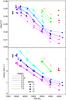 |
Fig. 6 Relative horizontal temperature fluctuation (top panel) and absolute vertical velocity fluctuations (bottom panel) at Rosseland optical depth τ = 2/3 in the 3D models. The surface gravity is color coded, metallicity is depicted by different plot symbols. |
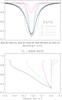 |
Fig. 7 Line profiles and velocity bisectors for the Fe I transition at 868.6 nm. The filled circles in the upper panel correspond to solar observations. Solid lines are for 3D simulations and broken lines for 1D models. Note that the 1D calculation at solar-metallicity for this line (broken solid line) shows a non-zero velocity bisector, due to overlapping CN transitions included in all our calculations that distort the otherwise perfectly symmetric 1D profiles. |
The filled circles in the upper panel of Fig. 7 show the renormalized observations for the Sun of Kurucz et al. (1984). A significant improvement in the agreement between theory and observation is obvious for the line core when going from 1D to 3D models (dashed and solid black lines, respectively). A similar effect is found using a Kurucz model, instead of its LHD counterpart, for the 1D spectrum. It is also noticeable the extreme discrepancies between the 1D and 3D cases at [Fe/H] = −2, as it is the large reduction in strength for the line calculated in 3D between [Fe/H] = −2 and −3. An exhaustive check of these predictions against high quality observations of metal-poor stars is very much needed.
Our calculations are likely least reliable for cool giants, and in fact the predicted convective shifts for stars approaching 4000 K are unlikely to be realistic. Gray et al. (2008) examined bisectors for a number of red giant stars with low metallicity, finding that those with temperatures of about 4100 K or less tend to exhibit reversed bisectors (with an “inverse C” shape, rather than with a “C”-like shape seen in solar-type stars). More recent results for the supergiant γ Cyg confirm the same trend (Gray 2010). These stars also tend to exhibit radial velocity “jitter” (see, e.g., Carney et al. 2008, and the theoretical predictions by Chiavassa et al. 2011b).
We have identified an expression that can reproduce the net convective blueshifts theoretically predicted for the RVS observations in Table 1 with an rms of 0.021 km s-1; and a maximum deviation of 0.074 km s-1. We have coded this expression into an IDL function provided in the appendix.
5. Gravitational redshifts
Photons escaping from a stellar photosphere to infinity are redshifted as a result of climbing up the gravitational field by GcM/R, where G is the Gravitational constant, c the speed of light, M the stellar mass, and R the stellar radius. Using solar units for the stellar mass and radius, the gravitational redshift amounts to 0.6365 M/R km s-1, and for light intercepted at 1 AU 0.6335 M/R km s-1 (Lindegren & Dravins 2003). The same effect acts when photons enter in the Earth’s gravitational field, which reduces the redshift by about 0.2 m s-1, but this small correction can be ignored for most purposes. With the parallaxes and spectrophotometry provided by Gaia, it should be possible to obtain fairly accurate customized predictions for the gravitational redshifts for individual Gaia targets.
Gravitational shifts for late-type dwarfs amount to about 0.7−0.8 km s-1 at log g ~ 4.5, but they dramatically decrease with surface gravity down to 0.02−0.03 km s-1 for the giants in our grid (log g ~ 1.5).
6. Discussion and summary
The radial velocities inferred from the wavelength shifts measured in stellar spectra are systematically offset from the true space velocities of stars projected along the line of sight due to a number of effects. Quantifying the impact of such effects is model dependent, and therefore the IAU has introduced the term “radial-velocity measure” (Lindegren & Dravins 2003) to refer to the radial velocity naively inferred from the relative wavelength shifts of lines cδλ/λ, and encourages observers to keep measurements disentangled from subsequent corrections2. Nevertheless, for most stars, two relatively clean corrections are dominant: photospheric gravitational redshifts and convective blueshifts. In the case of stars moving at high speed in the direction perpendicular to the observer, the relativistic contribution to the Dopper shift needs to be considered at a precision level of hundred of meters per second; the spectrum of a star with a transverse velocity of 300 km s-1 and no radial velocity will be redshifted as much as that of a star with a receding radial velocity of 0.15 km s-1.
We have used three-dimensional radiative-hydrodynamical simulations of surface convection in late-type stars to evaluate the impact of convective shifts on the spectra from the Radial Velocity Spectrometer onboard Gaia. The net velocity shifts derived by cross-correlation depend both on the wavelength range and the spectral resolution of the observations. Our models predict very small net convective shifts for the RVS observations of K-type stars, which increase with effective temperature to reach bout 0.3 km s-1 for F-type dwarfs. The predicted shifts depend as well on metallicity and surface gravity.
In the case of the Gaia mission, the corrections discussed above, which are <1 km s-1 are small in comparison with the typical uncertainties in the space velocities determined for individual stars, but can cause systematic errors when average values are derived for ensembles of stars. Even more important, since the Gaia RVS is a self-calibrated instrument, in the sense that the wavelength solution is derived from stellar observations, systematic offsets from star to star such as those related to convective shifts, need to be accounted for in the data reduction. In this paper, we used a grid of 3D hydrodynamical simulations to estimate convective blueshifts for stars with spectral types F to M, at different metallicities and evolutionary stages. We note that from data provided by Gaia itself, it will be possible to constrain the stellar masses and radii for individual stars, and therefore the gravitational redshifts.
Gravitational redshifts dominate convective blueshifts predicted for the Gaia window for dwarfs of all temperatures, in particular for later spectral types (K and M), where the convective shifts are weakest. Gravitational redshifts become weaker for stars with lower gravities. The opposite tendency, if less pronounced, is expected for the convective blueshifts, in such a way that gravitational and convective shifts nearly cancel each other for stars with intermediate gravities.
When adding together convective and gravitational shifts, we expect the largest velocity offset for the coolest dwarfs in our study, with effective temperatures around 4000 K, where the net effect, dominated by gravitational redshifts, amounts up to nearly 0.6 km s-1. By using the corrections provided here and custom-made estimates of the gravitational shifts, these sources of systematic error should be reduced significantly to a level ranging from about 0.1 km s-1 for F-type dwarfs, to a few tens of meters per second for late-K-type stars.
In addition to calculated convective shifts, we provide FITS files including the 1D and 3D model fluxes we have computed. These may turn useful to build radial velocity templates for derivation of radial velocities from observations.
We end with a word of caution. The theoretical calculations presented here only have been checked against a limited set of observations, mainly for the Sun. An exhaustive check against high-quality observed spectra for warmer and cooler temperatures, especially at very low metallicity, is still needed before one can ensure that the predicted shifts are completely trustworthy.
Online material
Appendix A: An empirical fitting function to describe the blueshifts as a function of atmospheric parmeters
To derive from the tabulated data an easily applicable function we follow the recursive fitting procedure outlined by Sbordone et al. (2010): we searched for an analytical function for the convective blueshift with three independent parameters (log Teff, log g and [Fe/H]), written as y = y(x0,x1,x2;A). The function and the vector of free parameters A = (A0,A1,...) that give the best fit to the tabulated data is to be found.
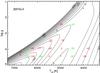 |
Fig. A.1 Convective shifts for solar metallicity simulations (in units of m s-1). The contours join the locations with the same convective blueshift, as predicted by our analytical fitting function. Red/green color is used in the regions where the analytical function under/over predicts the measurements performed on the simulations. |
The function-find routine (“fufi”, written in IDL) starts with the most simple “function”, a constant A0 – the weighted average of the tabulated blueshift data. At each recursive iteration we let the routine replace each parameter Ai of a candidate fitting function with a polynomial Ai → A0 + A1x0 + A2x1 + A3x2 or, alternatively, an exponential Ai → A0 + A1exp(A2 + A3x0 + A4x1 + A5x2) to reach the next level of complexity. For each of these functions, the optimum parameter set is then searched, using the parameters from the previous level as starting point. We use the inverse of the rms fluctuations of the convective shifts between the snapshots for a given stellar parameter combination (or 0.01 km s-1 when the fluctuations are below this value) as fitting weights. The function with the fitting-parameter set that provides the smallest overall error (among thousands of candidates) is finally written to a file as a Fortran or IDL function. The function we supply has been slightly edited to improve readability. We emphasize that the functional form and fitting parameters have no physical meaning whatsoever.
We varied some control parameters (the list of candidate terms and the recursion depth), and compared errors and the overall functional dependence of the results. Fitting functions composed exclusively of simple polynomial terms already give decent fits (and would require a much simpler procedure to derive than the one outlined above). Still, fits including the exponential term are superior and behave much better and closer to our expectations at – and even slightly beyond – the borders of the set of stellar parameters for which model results are available. The overall rms scatter between the direct measurements from the simulations and the fitting formula is just 0.021 km s-1, with a maximum deviation of 0.074 km s-1. We give an implementation of the fitting function in IDL below. It includes a check that the input parameters are within the range covered by the 3D models. A few of the free fitting parameters are zero, but are left in the routine to allow for a more systematic writing of the final expression. Figures A.1−A.4 illustrate the convective shifts predicted by the fitting equation for [Fe/H] = 0, −1,−2, and −3, respectively.
function ConvShift, Teff, logg, FeH
;
; IN: Teff – effective temperature (K)
; logg – surface gravity (g in cm/s2)
; FeH – [Fe/H] metallicity relative to solar
;
; OUT: Convective shift (m/s)
; (<0 for blueshifts)
;
; –- Thu Oct 20 20:09:50 2011 –- B.F. –-
;check that 3 parameters are input
if n_params() lt 3 then begin
print,’
return,-10000000000.d0
endif
;check that we’re within limits
if (min(Teff) lt 3790.00 or $
max(Teff) gt 6730.00 or $
min(FeH) lt -3.0 or $
max(FeH) gt 0. or $
max(logg) gt 4.5 or $
min(logg-(teff*9.184e-4-2.482)) lt 0.0) $
then begin
print,’% ConvShift: Params. out of range:’
print,’% 3790 <= Teff <= 6730. K’
print,’% 9.184e-4*Teff-2.482<=logg<= 4.5’
print,’% -3.0 <= [Fe/H] <= 0.0 dex’
return,-10000000000.d0
endif
logTeff=alog10(Teff*1d-3)
M=-FeH
A=dindgen(24)
A(00)= 3.9921954E-01 & A(01)=-7.1438992E-01
A(02)= 2.0028012E-02 & A(03)=-5.2146580E-02
A(04)=-4.1100047E-06 & A(05)= 0.0000000E+00
A(06)= 2.2334658E+01 & A(07)=-1.7070215E+00
A(08)=-1.7445524E-01 & A(09)= 1.4332379E-02
A(10)= 0.0000000E+00 & A(11)=-1.3239030E+01
A(12)= 8.2077384E-01 & A(13)=-9.6311294E-02
A(14)=-1.7150490E+03 & A(15)= 0.0000000E+00
A(16)=-9.3405848E+00 & A(17)= 7.7603954E-01
A(18)= 1.3519228E+00 & A(19)=-5.0111694E+00
A(20)= 0.0000000E+00 & A(21)=-8.2077414E-01
A(22)= 1.0457402E-01 & A(23)= 4.2118204E-01
Shift=A(00)+A(01)*logTeff+(A(02) + $ (A(04)+A(09)*exp(A(10)+(A(11)+ $
A(14)*exp(A(15)+ $ (A(16)+A(19)*exp(A(20)+ $
A(21)*logTeff+ $ A(22)*logg+ A(23)*M))*logTeff+ $
A(17)*logg+A(18)*M))*logTeff+ $ A(12)*logg+A(13)*M))*exp(A(05)+ $
A(06)*logTeff+A(07)*logg+A(08)*M))*logg+A(03)*M
Shift=-Shift
return, Shift
end
Predicted convective line shifts.
We note that the “radial-velocity measure” does not have a unique definition, since the value derived depends on the spectral features and the actual method used. Therefore, such measures must be accompanied by a detailed description of the procedure used to derive it.
Acknowledgments
We are indebted to Ivan Hubeny for assistance computing radiative opacities. Carlos Allende Prieto is thankful to Mark Cropper, David Katz, and Frédéric Thévenin for fruitful discussions. B.F. acknowledges financial support from the Agence Nationale de la Recherche (ANR), and the “Programme National de Physique Stellaire” (PNPS) of CNRS/INSU, France. HGL acknowledges financial support by the Sonderforschungsbereich SFB 881 “The Milky Way System” (subproject A4) of the German Research Foundation (DFG). The authors acknowledge the Texas Advanced Computing Center (TACC) at The University of Texas at Austin for providing H.P.C. resources that have contributed to the research results reported within this paper (http://www.tacc.utexas.edu).
References
- Abramowitz, M., Stegun, I. A., eds. 1972, Handbook of Mathematical Functions with Formulas, Graphs, and Mathematical Tables (New York: Dover Publications) [Google Scholar]
- Allen de Prieto, C. 2007, AJ, 134, 1843 [NASA ADS] [CrossRef] [Google Scholar]
- Allende Prieto, C., & GarciaLopez, R. J. 1998, A&AS, 129, 41 [NASA ADS] [CrossRef] [EDP Sciences] [Google Scholar]
- Allen de Prieto, C., & Lambert, D. L. 1999, A&A, 352, 555 [NASA ADS] [Google Scholar]
- Allende Prieto, C., García López, R. J., Lambert, D. L., & Gustafsson, B. 1999, ApJ, 526, 991 [NASA ADS] [CrossRef] [Google Scholar]
- Allen de Prieto, C., Koesterke, L., Ramírez, I., Ludwig, H.-G., & Asplund, M. 2009, Mem. Soc. Astron. It., 80, 622 [NASA ADS] [Google Scholar]
- Asplund, M. 2005, ARA&A, 43, 481 [NASA ADS] [CrossRef] [Google Scholar]
- Asplund, M., Nordlund, Å., Trampedach, R., Allen de Prieto, C., & Stein, R. F. 2000, A&A, 359, 729 [NASA ADS] [Google Scholar]
- Asplund, M., Grevesse, N., & Sauval, A. J. 2005, in Cosmic Abundances as Records of Stellar Evolution and Nucleosynthesis, eds. T. G. Barnes III, & F. N. Bash (San Francisco: ASP), 336, 25 [Google Scholar]
- Bigot, L., & Thévenin, F. 2006, MNRAS, 372, 609 [NASA ADS] [CrossRef] [Google Scholar]
- Bigot, L., & Thévenin, F. 2008, SF2A-2008, 3 [Google Scholar]
- de Bruijne, J. H. J. 2012, Ap&SS, 341, 31 [NASA ADS] [CrossRef] [Google Scholar]
- de Bruijne, J. H. J., Escolar, D., & Erdmann, M. 2009, SF2A-2009: Proceedings of the Annual meeting of the French Society of Astronomy and Astrophysics, 41 [Google Scholar]
- Caffau, E., & Ludwig, H.-G. 2007, A&A, 467, L11 [NASA ADS] [CrossRef] [EDP Sciences] [Google Scholar]
- Carney, B. W., Latham, D. W., Stefanik, R. P., & Laird, J. B. 2008, AJ, 135, 196 [NASA ADS] [CrossRef] [Google Scholar]
- Castelli, F., & Kurucz, R. L. 2004, Proc. IAU Symp. 210, Modelling of Stellar Atmospheres, eds. N. Piskunov et al. 2003, poster A20 [Google Scholar]
- Chiavassa, A., Bigot, L., Thévenin, F., et al. 2011a, J. Phys. Conf. Ser., 328, 012012 [NASA ADS] [CrossRef] [Google Scholar]
- Chiavassa, A., Pasquato, E., Jorissen, A., et al. 2011b, A&A, 528, A120 [NASA ADS] [CrossRef] [EDP Sciences] [Google Scholar]
- Collet, R., Asplund, M., & Trampedach, R. 2007, A&A, 469, 687 [NASA ADS] [CrossRef] [EDP Sciences] [Google Scholar]
- Grevesse, N., & Sauval, A. J. 1998, Space Sci. Rev., 85, 161 [NASA ADS] [CrossRef] [Google Scholar]
- Dravins, D., & Nordlund, A. 1990a, A&A, 228, 184 [NASA ADS] [Google Scholar]
- Dravins, D., & Nordlund, A. 1990b, A&A, 228, 203 [NASA ADS] [Google Scholar]
- Dravins, D., Lindegren, L., Nordlund, A., & Vandenberg, D. A. 1993, ApJ, 403, 385 [NASA ADS] [CrossRef] [Google Scholar]
- Feautrier, P. 1964, SAO Spec. Rep., 167, 80 [Google Scholar]
- Freytag, B., Steffen, M., & Dorch, B. 2002, Astron. Nachr., 323, 213 [NASA ADS] [CrossRef] [EDP Sciences] [Google Scholar]
- Freytag, B., Steffen, M., Ludwig, H.-G., et al. 2011, J. Comput. Phys., 231, 919 [Google Scholar]
- Gray, D. F. 1986, PASP, 98, 319 [NASA ADS] [CrossRef] [Google Scholar]
- Gray, D. F. 1992, The Observation and Analysis of Stellar Photospheres, Camb. Astrophys. Ser., 20 [Google Scholar]
- Gray, D. F. 2009, ApJ, 697, 1032 [NASA ADS] [CrossRef] [Google Scholar]
- Gray, D. F. 2010, AJ, 140, 1329 [NASA ADS] [CrossRef] [Google Scholar]
- Gray, D. F., Carney, B. W., & Yong, D. 2008, AJ, 135, 2033 [NASA ADS] [CrossRef] [Google Scholar]
- Gustafsson, B., Edvardsson, B., Eriksson, K., et al. 2008, A&A, 486, 951 [NASA ADS] [CrossRef] [EDP Sciences] [Google Scholar]
- Hinkle, K., Wallace, L., Valenti, J., & Harmer, D. 2000, Visible and Near Infrared Atlas of the Arcturus Spectrum 3727−9300 A, eds. K. Hinkle, L. Wallace, J. Valenti, & D. Harmer (San Francisco: ASP) [Google Scholar]
- Irwin, A. W. 1981, ApJS, 45, 621 [NASA ADS] [CrossRef] [Google Scholar]
- Katz, D., Munari, U., Cropper, M., et al. 2004, MNRAS, 354, 1223 [NASA ADS] [CrossRef] [Google Scholar]
- Katz, D., Cropper, M., Meynadier, F., et al. 2011, EAS Publ. Ser., 45, 189 [Google Scholar]
- Koesterke, L. 2009, AIP Conf. Ser., 1171, 73 [Google Scholar]
- Koesterke, L., Allen de Prieto, C., & Lambert, D. L. 2008, ApJ, 680, 764 [NASA ADS] [CrossRef] [Google Scholar]
- Kurucz, R. L., Furenlid, I., Brault, J., & Testerman, L. 1984, National Solar Observatory Atlas, Sunspot (New Mexico: National Solar Observatory) [Google Scholar]
- Lindegren, L. 2010, IAU Symp., 261, 296 [Google Scholar]
- Lindegren, L., & Dravins, D. 2003, A&A, 401, 1185 [NASA ADS] [CrossRef] [EDP Sciences] [Google Scholar]
- Ludwig, H.-G., Caffau, E., Steffen, M., et al. 2009, Mem. Soc. Astron. It., 80, 711 [NASA ADS] [Google Scholar]
- Nordlund, A. 1982, A&A, 107, 1 [NASA ADS] [Google Scholar]
- Nordlund, A., & Dravins, D. 1990, A&A, 228, 155 [NASA ADS] [Google Scholar]
- Pasquini, L., Melo, C.,Chavero, C., et al. 2011, A&A, 526, A127 [NASA ADS] [CrossRef] [EDP Sciences] [Google Scholar]
- Pierce, A. K., & Lopresto, J. C. 2000, Sol. Phys., 196, 41 [NASA ADS] [CrossRef] [Google Scholar]
- Ramírez, I., & Allen de Prieto, C. 2011, ApJ, 743, 135 [NASA ADS] [CrossRef] [Google Scholar]
- Ramírez, I., Allen de Prieto, C., & Lambert, D. L. 2008, A&A, 492, 841 [NASA ADS] [CrossRef] [EDP Sciences] [Google Scholar]
- Sbordone, L., Bonifacio, P., Caffau, E., et al. 2010, A&A, 522, A26 [NASA ADS] [CrossRef] [EDP Sciences] [Google Scholar]
- Stix, M. 2004, The Sun: an Introduction, 2nd edn., by Michael Stix. Astronomy and astrophysics library (Berlin: Springer) [Google Scholar]
- Tsuji, T. 1973, A&A, 23, 411 [NASA ADS] [Google Scholar]
- Wedemeyer, S., Freytag, B., Steffen, M., Ludwig, H.-G., & Holweger, H. 2004, A&A, 414, 1121 [NASA ADS] [CrossRef] [EDP Sciences] [Google Scholar]
- Wilkinson, M. I., Vallenari, A., Turun, C., et al. 2005, MNRAS, 359, 1306 [NASA ADS] [CrossRef] [Google Scholar]
All Tables
All Figures
|
Fig. 1 Observed (black line) and synthetic (1D in red, 3D in blue) spectra for Arcturus and the Sun – all data smoothed with a Gaussian kernel to have a resolving power of about 11 500 as appropriate for the Gaia RVS. Both the normalized spectra and the residuals are shown for each star. A microturbulence of 1.5 km s-1 was adopted for the 1D models, which were calculated with the LHD package. |
| In the text | |
|
Fig. 2 Spectra for a single snapshot of model d3t59g45mm00n01 (black) and its 1D counterpart (black), with near solar atmospheric parameters, are shown in the left-hand panels for two different values of the resolving power (R). The right-hand panels illustrate how the corresponding shifts (1D relative to 3D) are obtained by fitting the peak of the cross-correlation function with a parabola. |
| In the text | |
|
Fig. 3 Derived convective shift for model d3t59g45mm00n01, with near solar atmospheric parameters, as a function of the resolving power. These shifts are obtained by cross-correlation using the Gaia RVS spectral window, and fitting the peak of the cross-correlation function with a parabola. The dashed vertical line marks the RVS resolving power. |
| In the text | |
|
Fig. 4 Effective convective shifts predicted by the 3D hydrodynamical models for Gaia RVS observations. |
| In the text | |
|
Fig. 5 Three uppermost panels: predicted convective shifts and atmospheric parameters of the 3D hydrodynamical models for Gaia RVS observations. Two lowermost panels: convective shifts versus relative horizontal temperature fluctuations and the rms of the vertical velocity at Rosseland optical depth τ = 2/3. In all panels data points are color coded by metallicity as in Fig. 4. |
| In the text | |
|
Fig. 6 Relative horizontal temperature fluctuation (top panel) and absolute vertical velocity fluctuations (bottom panel) at Rosseland optical depth τ = 2/3 in the 3D models. The surface gravity is color coded, metallicity is depicted by different plot symbols. |
| In the text | |
|
Fig. 7 Line profiles and velocity bisectors for the Fe I transition at 868.6 nm. The filled circles in the upper panel correspond to solar observations. Solid lines are for 3D simulations and broken lines for 1D models. Note that the 1D calculation at solar-metallicity for this line (broken solid line) shows a non-zero velocity bisector, due to overlapping CN transitions included in all our calculations that distort the otherwise perfectly symmetric 1D profiles. |
| In the text | |
|
Fig. A.1 Convective shifts for solar metallicity simulations (in units of m s-1). The contours join the locations with the same convective blueshift, as predicted by our analytical fitting function. Red/green color is used in the regions where the analytical function under/over predicts the measurements performed on the simulations. |
| In the text | |
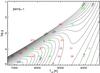 |
Fig. A.2 Convective shifts, [M/H] =-1. Similar to Fig. A.1. |
| In the text | |
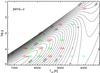 |
Fig. A.3 Convective shifts, [M/H] = −2. Similar to Fig. A.1. |
| In the text | |
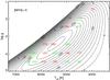 |
Fig. A.4 Convective shifts, [M/H] = −3. Similar to Fig. A.1. |
| In the text | |
Current usage metrics show cumulative count of Article Views (full-text article views including HTML views, PDF and ePub downloads, according to the available data) and Abstracts Views on Vision4Press platform.
Data correspond to usage on the plateform after 2015. The current usage metrics is available 48-96 hours after online publication and is updated daily on week days.
Initial download of the metrics may take a while.