| Issue |
A&A
Volume 550, February 2013
|
|
|---|---|---|
| Article Number | A103 | |
| Number of page(s) | 13 | |
| Section | Stellar atmospheres | |
| DOI | https://doi.org/10.1051/0004-6361/201220064 | |
| Published online | 04 February 2013 | |
Online material
Appendix A: An empirical fitting function to describe the blueshifts as a function of atmospheric parmeters
To derive from the tabulated data an easily applicable function we follow the recursive fitting procedure outlined by Sbordone et al. (2010): we searched for an analytical function for the convective blueshift with three independent parameters (log Teff, log g and [Fe/H]), written as y = y(x0,x1,x2;A). The function and the vector of free parameters A = (A0,A1,...) that give the best fit to the tabulated data is to be found.
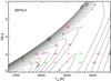 |
Fig. A.1
Convective shifts for solar metallicity simulations (in units of m s-1). The contours join the locations with the same convective blueshift, as predicted by our analytical fitting function. Red/green color is used in the regions where the analytical function under/over predicts the measurements performed on the simulations. |
| Open with DEXTER | |
The function-find routine (“fufi”, written in IDL) starts with the most simple “function”, a constant A0 – the weighted average of the tabulated blueshift data. At each recursive iteration we let the routine replace each parameter Ai of a candidate fitting function with a polynomial Ai → A0 + A1x0 + A2x1 + A3x2 or, alternatively, an exponential Ai → A0 + A1exp(A2 + A3x0 + A4x1 + A5x2) to reach the next level of complexity. For each of these functions, the optimum parameter set is then searched, using the parameters from the previous level as starting point. We use the inverse of the rms fluctuations of the convective shifts between the snapshots for a given stellar parameter combination (or 0.01 km s-1 when the fluctuations are below this value) as fitting weights. The function with the fitting-parameter set that provides the smallest overall error (among thousands of candidates) is finally written to a file as a Fortran or IDL function. The function we supply has been slightly edited to improve readability. We emphasize that the functional form and fitting parameters have no physical meaning whatsoever.
We varied some control parameters (the list of candidate terms and the recursion depth), and compared errors and the overall functional dependence of the results. Fitting functions composed exclusively of simple polynomial terms already give decent fits (and would require a much simpler procedure to derive than the one outlined above). Still, fits including the exponential term are superior and behave much better and closer to our expectations at – and even slightly beyond – the borders of the set of stellar parameters for which model results are available. The overall rms scatter between the direct measurements from the simulations and the fitting formula is just 0.021 km s-1, with a maximum deviation of 0.074 km s-1. We give an implementation of the fitting function in IDL below. It includes a check that the input parameters are within the range covered by the 3D models. A few of the free fitting parameters are zero, but are left in the routine to allow for a more systematic writing of the final expression. Figures A.1−A.4 illustrate the convective shifts predicted by the fitting equation for [Fe/H] = 0, −1,−2, and −3, respectively.
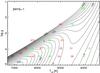 |
Fig. A.2
Convective shifts, [M/H] =-1. Similar to Fig. A.1. |
| Open with DEXTER | |
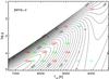 |
Fig. A.3
Convective shifts, [M/H] = −2. Similar to Fig. A.1. |
| Open with DEXTER | |
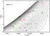 |
Fig. A.4
Convective shifts, [M/H] = −3. Similar to Fig. A.1. |
| Open with DEXTER | |
function ConvShift, Teff, logg, FeH
;
; IN: Teff – effective temperature (K)
; logg – surface gravity (g in cm/s2)
; FeH – [Fe/H] metallicity relative to solar
;
; OUT: Convective shift (m/s)
; (<0 for blueshifts)
;
; –- Thu Oct 20 20:09:50 2011 –- B.F. –-
;check that 3 parameters are input
if n_params() lt 3 then begin
print,’
return,-10000000000.d0
endif
;check that we’re within limits
if (min(Teff) lt 3790.00 or $
max(Teff) gt 6730.00 or $
min(FeH) lt -3.0 or $
max(FeH) gt 0. or $
max(logg) gt 4.5 or $
min(logg-(teff*9.184e-4-2.482)) lt 0.0) $
then begin
print,’% ConvShift: Params. out of range:’
print,’% 3790 <= Teff <= 6730. K’
print,’% 9.184e-4*Teff-2.482<=logg<= 4.5’
print,’% -3.0 <= [Fe/H] <= 0.0 dex’
return,-10000000000.d0
endif
logTeff=alog10(Teff*1d-3)
M=-FeH
A=dindgen(24)
A(00)= 3.9921954E-01 & A(01)=-7.1438992E-01
A(02)= 2.0028012E-02 & A(03)=-5.2146580E-02
A(04)=-4.1100047E-06 & A(05)= 0.0000000E+00
A(06)= 2.2334658E+01 & A(07)=-1.7070215E+00
A(08)=-1.7445524E-01 & A(09)= 1.4332379E-02
A(10)= 0.0000000E+00 & A(11)=-1.3239030E+01
A(12)= 8.2077384E-01 & A(13)=-9.6311294E-02
A(14)=-1.7150490E+03 & A(15)= 0.0000000E+00
A(16)=-9.3405848E+00 & A(17)= 7.7603954E-01
A(18)= 1.3519228E+00 & A(19)=-5.0111694E+00
A(20)= 0.0000000E+00 & A(21)=-8.2077414E-01
A(22)= 1.0457402E-01 & A(23)= 4.2118204E-01
Shift=A(00)+A(01)*logTeff+(A(02) + $ (A(04)+A(09)*exp(A(10)+(A(11)+ $
A(14)*exp(A(15)+ $ (A(16)+A(19)*exp(A(20)+ $
A(21)*logTeff+ $ A(22)*logg+ A(23)*M))*logTeff+ $
A(17)*logg+A(18)*M))*logTeff+ $ A(12)*logg+A(13)*M))*exp(A(05)+ $
A(06)*logTeff+A(07)*logg+A(08)*M))*logg+A(03)*M
Shift=-Shift
return, Shift
end
Predicted convective line shifts.
© ESO, 2013
Current usage metrics show cumulative count of Article Views (full-text article views including HTML views, PDF and ePub downloads, according to the available data) and Abstracts Views on Vision4Press platform.
Data correspond to usage on the plateform after 2015. The current usage metrics is available 48-96 hours after online publication and is updated daily on week days.
Initial download of the metrics may take a while.