| Issue |
A&A
Volume 550, February 2013
|
|
|---|---|---|
| Article Number | A42 | |
| Number of page(s) | 23 | |
| Section | Interstellar and circumstellar matter | |
| DOI | https://doi.org/10.1051/0004-6361/201219682 | |
| Published online | 22 January 2013 | |
Three-dimensional interstellar extinction map toward the Galactic bulge⋆,⋆⋆
1
Institut Utinam, CNRS UMR 6213, OSU THETA, Université de Franche-Comté,
41bis avenue de l’Observatoire
25000
Besançon
France
e-mail: This email address is being protected from spambots. You need JavaScript enabled to view it.
; This email address is being protected from spambots. You need JavaScript enabled to view it.
;
This email address is being protected from spambots. You need JavaScript enabled to view it.
2
Department of Astronomy, Beijing Normal University,
100875
Beijing, PR
China
e-mail: This email address is being protected from spambots. You need JavaScript enabled to view it.
3
Institut d’Astrophysique de Paris, UMR 7095 CNRS, Université
Pierre et Marie Curie, 98bis
boulevard Arago, 75014
Paris,
France
4
European Southern Observatory, Karl-Schwarzschild-Strasse 2, 85748
Garching,
Germany
e-mail: This email address is being protected from spambots. You need JavaScript enabled to view it.
; This email address is being protected from spambots. You need JavaScript enabled to view it.
5
Departamento Astronomía y Astrofísica, Pontificia Universidad
Católica de Chile, Av. Vicuña
Mackenna 4860, Stgo., Chile
e-mail: This email address is being protected from spambots. You need JavaScript enabled to view it.
6 Vatican Observatory, V00120, Vatican City State
Received:
25
May
2012
Accepted:
13
November
2012
Abstract
Context. Studies of the properties of the inner Galactic bulge strongly depend on the assumptions made about interstellar extinction. Most of the extinction maps available in the literature lack the information about the distance.
Aims. We combine observations with the Besançon model of the Galaxy to investigate the variations of extinction along different lines of sight toward the inner Galactic bulge as a function of distance. In addition we study the variations in the extinction law in the bulge.
Methods. We constructed color–magnitude diagrams with the following sets of colors: H–Ks and J–Ks from the VVV catalog and Ks–[3.6], Ks–[4.5], Ks–[5.8] and Ks–[8.0] from GLIMPSE-II catalog matched with 2MASS. Using the newly derived temperature−color relation for M giants that match the observed color–magnitude diagrams better we then used the distance−color relations to derive the extinction as a function of distance. The observed colors were shifted to match the intrinsic colors in the Besançon model as a function of distance, thereby iteratively creating an extinction map with three dimensions: two spatial and one distance dimension along each line of sight toward the bulge.
Results. Color excess maps are presented at a resolution of 15′ × 15′ for six different combinations of colors in distance bins of 1 kpc. The high resolution and depth of the photometry allows us to derive extinction maps to 10 kpc distance and up to 35 mag of extinction in AV (3.5 mag in AKs). Integrated maps show the same dust features and consistent values with the other 2D maps. Starting from the color excess between the observations and the model, we investigate the extinction law in near-infrared and its variation along different lines of sight.
Key words: dust, extinction / Galaxy: bulge / Galaxy: stellar content / Galaxy: structure
Appendices are available in electronic form at http://www.aanda.org
Full Tables 1 and 2 are only available in electronic form at the CDS via anonymous ftp to cdsarc.u-strasbg.fr (130.79.128.5) or via http://cdsarc.u-strasbg.fr/viz-bin/qcat?J/A+A/550/A42
© ESO, 2013
1. Introduction
Interstellar extinction is a serious obstacle for the interpretation of stellar populations in the Galactic bulge. It shows an in-homogeneous clumpy distribution and is extremely high toward the Galactic center.
Several studies of cumulative extinction at the distance of the inner Galactic bulge have been made: Schultheis et al. (1999) used the DENIS near-infrared data set in combination with theoretical red giant branch (RGB)/asymptotic giant branch (AGB) isochrones from Bertelli et al. (1994). They showed that for an appropriate sampling area the observed sequence matched the isochrone with appropriate reddening well. The highest extinction that could be reliably derived from the J and Ks data available from DENIS was about AV = 25m. Schultheis et al. (1999) found that in some areas, presumably those with the highest extinctions, no J-band counterparts for sources were detected in Ks. For these regions, only lower limits to the extinctions could be obtained. Dutra et al. (2003) obtained similar results using the same technique with 2MASS data. Gonzalez et al. (2011) mapped the extinction along the minor axis of the bulge based on the Vista Variables in the Via Lactea (VVV) ESO public survey data (Saito et al. 2012) using the red clump giants. Gonzalez et al. (2012) presented the full extinction map over the entire VVV data set covering 315 sq. degrees using the red clump technique. This map extends beyond the inner Milky Way bulge also to higher Galactic latitudes and is the most complete study extending up to AV ~ 35m, which are much higher extinction values than were used in most previous studies. Recently, Nidever et al. (2012) determined high-resolution AKs maps using GLIMPSE-I, GLIMPSE-II, and GLIMPSE-3d data based on the Rayleigh-Jeans color excess (RJCE) method.
However, most of the studies are restricted to 2D extinction maps. Drimmel et al. (2003) built a theoretical large-scale 3D Galactic dust extinction map. Marshall et al. (2006) presented a 3D model of the extinction properties of the Galaxy by using the 2MASS data and the stellar population synthesis model of the Galaxy, the so-called Besançon model of the Galaxy (Robin et al. 2003). However, Marshall et al.’s study is limited by the confusion limit of 2MASS in the Galactic bulge region and by the limiting sensitivity of 2MASS in highly extincted regions (AV > 30m). Recently, Robin et al. (2012) improved the Besançon model significantly by adding a bar component which results in an excellent agreement for a comparsion of 2MASS color–magnitude diagrams in the metallicity as well as for the radial velocity distribution (see Babusiaux et al. 2010; Gonzalez et al. 2012; Uttenthaler et al. 2012). We used this updated model to build a new 3D extinction model using the GLIMPSE-II data, which map the Galactic plane within ± 10 degrees in longitude from the Galactic center with a wavelength coverage between 3.6 to 8.0 μm, allowing one to map the most highly extincted regions, as shown in Schultheis et al. (2009). In addition, we used the recently published VVV data with a pixel size nearly ten times smaller and a sensitivity in Ks of 3–4 mag deeper than 2MASS to map the 3D extinction in the near infrared (IR).
The infrared color–color diagram J–Ks vs. K–[mid-IR] has been used by Jiang et al. (2006) and Indebetouw et al. (2005) to determine the extinction coefficients Amid−ir along different lines of sight. Gao et al. (2009) traced the extinction coefficients based on the data from the GLIMPSE survey and found systematic variations of the extinction coefficients with Galactic longitude, which appears to correlate with the location of the spiral arms. Zasowski et al. (2009) found a Galactic radial dependence of the extinction law in the mid-IR using GLIMPSE data, while Nishiyama et al. (2009) determined the extinction law close to the Galactic center between 1.2 and 8.0 μm.
In this paper, we first introduce our data set in Sect. 2. We discuss in Sect. 3 the Besançon stellar population synthesis model together with the recent improvements. In Sect. 4 we describe the method for determining the extinction coefficients, and in Sect. 5 the method deriving the 3D-extinction. We finish in Sect. 6 with the determination of the extinction coefficient part and the conclusion (Sect. 7).
2. Data set
2.1. GLIMPSE-II survey
The Galactic Legacy Infrared Mid-Plane Survey Experiment (GLIMPSE) surveyed about 20 square degrees of the central region of the Galactic inner bulge using the Spitzer Space Telescope (Werner et al. 2004) equipped with the Infrared Array Camera (IRAC) (Fazio et al. 2004). It surveyed approximately 220 square degrees of the Galactic plane at four IRAC bands [3.6], [4.5], [5.8], and [8.0], centered at approximately 3.6, 4.5, 5.8, and 8.0 μm. The GLIMPSE-II data cover a range of longitudes from −10° to 10° and a range of latitudes from ± 1 deg to ± 2 deg depending on the longitude. The GLIMPSE-II coverage does not include the Galactic center region |l| ≤ 1° and |b| ≤ 0.75°, which was observed by the GALCEN program (Ramírez et al. 2008).
We used here the point-source archive (GLMIIA, Churchwell et al. 2009). The GLMIIA catalogs consist of point sources with a signal-to-noise ratio higher than 5 in at least one band and less stringent selection criteria than the catalog (see Churchwell et al. 2009 for more information). It contains the entire GLIMPSE-II survey region including the GALCEN data and GLIMPSE-I data at the boundary of the surveys (at l = 10° and l = −10°). Moreover, these catalogs were also merged with 2MASS, resulting in a seven-band catalog: three 2MASS bands and four IRAC bands. The photometric uncertainty of the GLIMPSE-II data is typically better than 0.2 mag and the astrometric accuracy is better than 0.3′′.
2.2. VVV-survey data
The other data set comes from the VVV ESO VISTA near-IR public survey. Observations were carried out using the VIRCAM camera on the VISTA 4.1 m telescope (Emerson & Sutherland 2010) located at the ESO Cerro Paranal Observatory in Chile. The five-year-variability campaign of the survey, which started observations during 2010, will repeatedly observe in an area of ~564 deg2Ks-band , including a region of the Galactic plane from 295° < l < 350° to −2° < b < 2°, and the bulge spanning from −10° < l < 10° and −10° < b < +5°. During the first year of observations, the complete survey area was fully imaged in five bands: Z, Y, H, J, and Ks. In this work, we used the J, H, and Ks catalogs for the same field of the GLIMPSE-II data from the 314 sq.deg coverage of the Galactic bulge. For a complete description of the survey and the observation strategy we refer to Minniti et al. (2010). A detailed description of the data products used in this work, corresponding to the first VVV data release, can be found in Saito et al. (2012).
A description of the single-band photometric catalogs, produced by the Cambridge Astronomical Survey Unit (CASU), and the procedure to build the multi-band catalogs can be found in Gonzalez et al. (2011). These catalogs were used in Gonzalez et al. (2012) to construct the complete 2D extinction map of the bulge and are the same ones used for the present study. We provide here only a brief summary of the procedure. J, H, and Ks catalogs produced by the CASU are first matched using the STILTS (Taylor 2006) code based on the proximity of sky positions. Since VVV photometry is saturated for stars brighter than Ks = 12 mag, 2MASS photometry is used to complete the bright end of the catalogs. Therefore, VVV catalogs are calibrated into the 2MASS photometric system. As described in Gonzalez et al. (2011), this calibration zero point is obtained by matching VVV sources with those of 2MASS in the magnitude range of 12m < Ks < 13m. This magnitude range was selected to avoid the saturation limit of VVV and the faint 2MASS magnitudes with poor photometric quality. This last point is also supported by using only sources flagged with high photometric quality in the 2MASS catalogs. The calibration zero point is calculated and applied individually for each VVV tile catalog. The final J, H, and Ks magnitudes in the calibrated catalogs are in the usual 2MASS system.
2.3. Completeness limit
Owing to the different pixel sizes of the different surveys (GLIMPSE-II, 2MASS, and VVV), completeness limits change as a function of wavelength and depend on the field direction. We divided the GLIMPSE II fields into subfields of 15′ × 15′ each to ensure a sufficient number of stars (at least 200) for our fitting process (see Sect. 4). The completeness limit for every subfield was then calculated in each filter. To estimate the completeness we used star counts as a function of magnitude where the peak of each histogram in each filter gives the corresponding completeness limit. The catalog becomes severely incomplete beyond the point where the star counts are highest. We are aware that this is a simple treatment of the completeness limit. However, we also clearly see here how strongly the completeness limit changes along different lines of sight as demonstrated (Saito et al. 2012) using artificial sources.
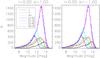 |
Fig. 1 Star counts of GLIMPSE-II data of two example fields for the 2MASS bands and IRAC bands. Each field is 15′ × 15′. |
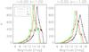 |
Fig. 2 Star counts of VVV-survey data of two example fields for the 2MASS bands. Each field is 15′ × 15′. |
Figure 1 shows the star counts as a function of magnitude for the GLIMPSE-II and 2MASS catalogs for two subfields, one located at (l, b) = (0, +1) which is our reference field (the so-called C32 field) because of its very homogeneous and low extinction (Omont et al. 1999, 2003). The second field is located at (l, b) = (0, −1) selected here for its higher and more clumpy extinction (Ojha et al. 2003). Due to crowding and extinction, the completeness limit can change within one or two magnitudes in the infrared bands. The difference in the completeness limit at [3.6] and [4.5] clearly visible, compared to [5.8] and [8.0] for both fields, indicating the higher sensitivity of [3.6] and [4.5].
Figure 2 shows the same fields, this time with star count histograms from the VVV data. Note the “artificial” rise at Ks = 12m, which is the upper brightness limit of VVV. We decided to use the VVV data only from Ks > 12m in the following analysis. Figure 2 demonstrates a clear gain in sensitivity of VVV in comparison with 2MASS near-IR photometry. As shown by Saito et al. (2012), the VVV data confusion are limited. However, because spatial scales of the two catalogs are not fully matched and because the overlap between 2MASS and VVV is in the magnitude range where the completeness between the two catalogs is very different, we did not investigate this problem in more depth (this is beyond the scope of this paper), but it should be kept in mind when assessing the results.
We divided the VVV data into the same subfields as in the GLIMPSE-II data set.
3. The Besançon model
3.1. Main description
The Besançon Galaxy model is a stellar population synthesis model of the Galaxy based on the scenario of formation and evolution of the Milky Way (Robin et al. 2003). It simulates the stellar contents of the Galaxy by using the four distinct stellar populations: the thin disk, the thick disk, the bulge, and the spheroid. It also takes into account the dark halo and a diffuse component of the interstellar medium. For each population, a star formation-rate history and initial mass function are assumed, which allows one to generate stellar catalogs for any given direction, and returns the magnitude, color, and distance for each simulated star as well as the kinematics and other stellar parameters. The model in its present form can simulate observations in many combinations of different photometric systems from the ultraviolet (UV) to the IR. The photometry is computed using stellar atmosphere models (Basel 3.1) from Lejeune et al. (1997) and (1998). However, while the Basel 3.1 stellar library is reliable for temperatures higher than 4000 K, atmospheric models become much more complex through the appearance of molecules such as TiO, VO, and H2O for cooler stars. Because we have a significant contribution of M giants in our study, we decided to adopt a more realistic Teff vs. color relation that extends to cooler objects of about 2500 K. This new relation is described in Sect. 3.2.
Recently, a new bulge model has been proposed by Robin et al. (2012) as the sum of two ellipsoids: a main component that is the standard boxy bulge/bar, which dominates the counts up to latitudes of about 5°, and a second ellipsoid that has a thicker structure seen mainly at higher latitudes. The resulting 2MASS color–magnitude diagrams as well as star counts of this two component model clearly indicate the significant improvement (see Robin et al. 2012). Uttenthaler et al. (2012) also showed an excellent agreement in the kinematics based on radial velocity measurements.
For more detailed information about the Besançon model we refer to Robin et al. (2003) and the most recent update in Robin et al. (2012).
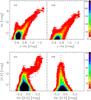 |
Fig. 3 Comparison of the the simulated color–magnitude diagrams using the old Teff vs. color relation (left) compared to the new one (right) for the reference field (l = 0.00 and b = 1.00). The color bar indicates the number of the stars. |
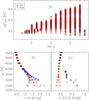 |
Fig. 4 a): log Teff vs. log g grid in the Besançon model. Black triangles indicate the coverage of the Besançon model (Robin et al. 2003) while red stars show the new extended grid. b): J–Ks vs. Teff relation. Black triangles show the old relation and red crosses the new one. The blue symbols is the relation for M giants from Houdashelt et al. (2000). c): Similar as b) but for K–[4.5] vs. Teff. |
3.2. Implementing IRAC colors and a new temperature–color relation
Reliable temperature–color relations are of extreme importance for comparing the synthetic color−magnitude and color–color diagrams with the observed ones. We used the reference field at (l, b) = (0, +1) to check the new synthetic colors in the [IRAC] filters. Figure 3 shows a kink in the Ks–[4.5] vs. [4.5] color−magnitude diagram at [Ks]−[4.5] ~ +0.1, [4.5] ~ 10, which we clearly identify also in the corresponding temperature vs. color relation (see Fig. 4c). While the Basel 3.1 library predicts decreasing J–Ks values for Teff < 3000 K, our new adopted relation shows a steady increase in J–Ks until Teff = 2500 K. We also noticed that the full parameter space in the log Teff vs. log g plane was not covered in the previous model, in particular, there is a gap in the temperature range between 2500–4000 K for 0.5 < log g < 3.
We updated the temperature–color relation and filled in the gap, using the isochrones from Girardi et al. (2010). These isochrones include the TP-AGB phase (Marigo et al. 2008) including mass-loss. Starting from a group of isochrones with ages ranging between 5–10 Gyr, we derived a new temperature vs. color relation for metallicities between [Fe/H] = −2 and [Fe/H] = 0.0. These ages and metallicities are characteristic of the bulge populations (e.g. Zoccali et al. 2003, 2008; Bensby et al. 2011). The comparison between the color−temperature relations from the Besançon model (so-called old relation) and the relation derived by us (so-called new relation) is shown in Figs. 4b and c. For comparison we show the J–Ks vs. Teff relation obtained by Houdashelt et al. (2000) for M giants. The clear difference between the new and old temperature vs. color relations for Teff < 4000 K is obviously responsible for the bent in the color−magnitude diagram (Fig. 3), which disappears after adopting our new relation. We also see that using the new relation the J–Ks colors will be systematically redder by about 0.05 mag.
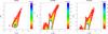 |
Fig. 5 Comparison of the Ks–[4.5] vs. [4.5] diagram of Baade window (left panel) with the old (middle panel) and the new temperature vs. color relation (left panel). The data are from Uttenthaler et al. (2010). The color bar indicates the number of the stars. |
Figure 5 shows the comparison of a color–magnitude diagram in a low-extinction field, the so-called Baade window. We used here the catalog of Uttenthaler et al. (2010). One clearly notices that the predicted color in the old model is too blue compared to the observations and we see in addition a much higher percentage of foreground objects (Ks− [4.5] < 0.5), which we do not find in the data.
4. Method
We obtained the extinction by using the color excess between the intrinsic color (derived
from the model defined as Coins) and the observational apparent color (derived
from the observation, here defined as Coobs). Assuming an extinction law, we
obtain:  (1)where
cλ is related to the extinction coefficient.
As we trace our fields close to the Galactic center, we used the extinction coefficients
from Nishiyama et al. (2009). We ignored here the
effect of the broadband extinctions and the reddenings on the spectral energy distribution
(SED) of the individual sources because our method does not allow for a more sophisticated
treatment, which could imply systematic errors. This results in
(1)where
cλ is related to the extinction coefficient.
As we trace our fields close to the Galactic center, we used the extinction coefficients
from Nishiyama et al. (2009). We ignored here the
effect of the broadband extinctions and the reddenings on the spectral energy distribution
(SED) of the individual sources because our method does not allow for a more sophisticated
treatment, which could imply systematic errors. This results in
![Mathematical equation: \begin{eqnarray*} &&A_{K{\rm s},J-K{\rm s}} = 0.528 \times ((J{-}K{\rm s})_{\rm obs}-(J{-}K{\rm s})_{\rm ins}) \\ && A_{K{\rm s},H-K{\rm s}} = 1.61 \times ((H{-}K{\rm s})_{\rm obs}-(H{-}K{\rm s})_{\rm ins}) \\ && A_{[3.6],K{\rm s}-[3.6]} = 1.005 \times ((K{\rm s}{-}[3.6])_{\rm obs}-(K{\rm s}{-}[3.6])_{\rm ins}) \\ && A_{[4.5],K{\rm s}-[4.5]} = 0.640 \times ((K{\rm s}{-}[4.5])_{\rm obs}-(K{\rm s}{-}[4.5])_{\rm ins}) \\ && A_{[5.8],K{\rm s}-[5.8]} = 0.562 \times ((K{\rm s}{-}[5.8])_{\rm obs}-(K{\rm s}{-}[5.8])_{\rm ins}) \\ && A_{[8.0],K{\rm s}-[8.0]} = 0.748 \times ((K{\rm s}{-}[8.0])_{\rm obs}-(K{\rm s}{-}[8.0])_{\rm ins}). \end{eqnarray*}](/articles/aa/full_html/2013/02/aa19682-12/aa19682-12-eq55.png) Below we apply the same
method as Marshall et al. (2006) assuming that the
distance grows as the apparent color/extinction increases. Figure 6b and c show an example of this relation for our reference field. In
contrast to Marshall et al. (2006), we used the full
information of the stellar populations in the color−magnitude diagram, that is, we also
included the M-dwarf population. While the local dwarf population
(d < 1–2 kpc) can be easily identified (see Marshall et al. 2006) by simple photometric color criteria (e.g.
J–Ks), this is not the case for dwarfs located at larger
distances where they cannot be separated from giants. This is especially true for the VVV
data where we are able to detect dwarf stars up to larger distances. However, the model
simulations show that the contribution of dwarf stars within the VVV completeness limit used
in our study is rather small (~1%) but can increase up to 20–30% going to fainter
magnitudes beyond the VVV completeness limit.
Below we apply the same
method as Marshall et al. (2006) assuming that the
distance grows as the apparent color/extinction increases. Figure 6b and c show an example of this relation for our reference field. In
contrast to Marshall et al. (2006), we used the full
information of the stellar populations in the color−magnitude diagram, that is, we also
included the M-dwarf population. While the local dwarf population
(d < 1–2 kpc) can be easily identified (see Marshall et al. 2006) by simple photometric color criteria (e.g.
J–Ks), this is not the case for dwarfs located at larger
distances where they cannot be separated from giants. This is especially true for the VVV
data where we are able to detect dwarf stars up to larger distances. However, the model
simulations show that the contribution of dwarf stars within the VVV completeness limit used
in our study is rather small (~1%) but can increase up to 20–30% going to fainter
magnitudes beyond the VVV completeness limit.
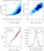 |
Fig. 6 Calculation process for the extinction of the example subfield (l, b) of (0.0, +1.0). From upper left to lower right, they are a) the errors of [3.6] vs. the [3.6] diagram, b) the color Ks–[3.6] vs. distance diagram, c) the extinction at [3.6] vs. the distance diagram where we show the first initial guess of extinction after the first iteration (black) and the final iteration after 20 loops, (red) and d) the color Ks–[3.6] distribution of the data compared to the first guess iteration (black) and the final one (red). |
Extinction as a function of Galactic longitude, latitude, and distance based on VVV data.
Extinction as a function of Galactic longitude, latitude, and distance based on GLIMPSE-II data.
The method can be described in following steps:
-
1.
First we add photometric errors and a diffuse extinction to theintrinsic colors Coins from the model for each subfield. The assumption of a diffuse extinction is necessary to ensure that the colors of the model increase with distance. We assume a diffuse extinction of 0.7 mag/kpc in the V band. We use exponential errors for the GLIMPSE-II data in all seven filters. Figure 6a shows an example of the photometric errors as a function of the [3.6] mag for our reference field (l, b) = (0.00, +1.00). The error is much smaller for the VVV data and we adopted a constant error of 0.05 mag (Saito et al. 2012). This procedure provides a first set of simulated colors (Cosim,ini)
-
2.
Colors are then sorted for observed and simulated data (Coobs and Cosim,ini), and normalized by the corresponding number of colors in each bin given by nbin = floor(min([Nobs,Nbes] )/100). Nobs and Nbes are the total number of observed stars (in each subfield) and of stars in the Besançon model. This ensures that we have at least 100 stars per bin.
-
3.
In each corresponding color bin, the Coins of the stars from the model data and the Coobs from the observational data are used to calculate the extinction using Eq. (1), as well as the median distance from the model. A first distance and extinction estimate can be thus obtained (A1st). Due to the saturation limit of VVV (Ks = 12), we do not get enough stars in the first distance bins (0–3 kpc). Therefore our 3D map starts at 4 kpc for VVV, and at 3 kpc for GLIMPSE-II data.
-
4.
The extinction and the distance estimated from the third step is then directly applied to the intrinsic magnitudes in the model, which gives us a new simulated color (Cosim,1 = Coins + A1st).
-
5.
We construct histograms for each color of the new simulated data (Cosim,1) and the observational data (Coins) using the same binsize (0.05 mag). The χ2 statistics (Press et al. 1992; Marshall et al. 2006) are then used to evaluate the similarity of the two histograms, given by
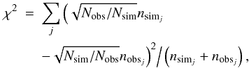 (2)where Nobs
and Nsim are the total number of observed and simulated
stars in each subfield, while
nobsj and
nsimj show the number of
stars for the jth color bin of the observations and simulated data.
With the first extinction estimate applied we now have a new set of simulated data.
For this new set of data, some of the stars may be fainter and fall outside the
completeness limit while others may be brighter and come inside the limit. We return
to the second step with the new Cosim,1 that would be used iteratively to
refine our results. In total we perform 20 iterations for each subfield and each
color. The minimum χ2 is then our final result. We have
chosen 20 loops to ensure that we always find a minimum value. In most of the cases
the χ2 converges after one or two loops to a minimum and
becomes stable in the following loops.
(2)where Nobs
and Nsim are the total number of observed and simulated
stars in each subfield, while
nobsj and
nsimj show the number of
stars for the jth color bin of the observations and simulated data.
With the first extinction estimate applied we now have a new set of simulated data.
For this new set of data, some of the stars may be fainter and fall outside the
completeness limit while others may be brighter and come inside the limit. We return
to the second step with the new Cosim,1 that would be used iteratively to
refine our results. In total we perform 20 iterations for each subfield and each
color. The minimum χ2 is then our final result. We have
chosen 20 loops to ensure that we always find a minimum value. In most of the cases
the χ2 converges after one or two loops to a minimum and
becomes stable in the following loops.
Figure 6c shows an example of the iteration process using the Ks–[3.6] color of the GLIMPSE-II data in our reference field (l, b) = (0.00, 1.00). We clearly see the difference between the first extinction estimate and our final extinction determination after 20 loops. We adapted the same completeness limit as in the observations for the model simulations (see Sect. 2.3).
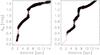 |
Fig. 7 Test of our method. The red line is the artificial extinction with clouds. The black crosses show our derived extinction values. The left panel is of field (l, b) = (0.00, +1.00) and the right of field (l, b) = (5.00, 0.00). |
To test our method, we used artificial data by manually adding extinction values to the intrinsic magnitude of the model. We used different lines of sight with a different number of clouds. Figure 7 shows two examples of several clouds. For field (l, b) at (0.00, 1.00), one located at a distance of 2 kpc with AV = 4.5 mag, the second one at 6 kpc with AV = 2.5 mag. For field (l, b) = (5.00, 0.00), we assumed three clouds: AV = 2.20 mag at 2.0 kpc, 2.50 mag at 5.0 kpc and 2.70 mag at 7.0 kpc. We applied our method to our simulated data. We found 328 000 sources for the first field and 182 000 for the second field. We artificially cut the data at Ks = 18 mag, which goes much deeper than the observational data. Figure 7 shows that our method successfully derives the extinction along the distance and that we are able to trace this multi-cloud structure. Modifying the input parameters of the Galactic model such as Galactic scale length, the size of the hole of the Galactic disk or changing the bulge luminosity function could lead to systematic differences in our derived extinction map. But this systematics, as shown in Marshall et al. (2006), is on the order of the random uncertainty of the method.
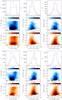 |
Fig. 8 Color–magnitude diagram and color distribution for all colors of the field l = 0.00, b = 1.00. The lower panel shows the observed color–magnitude diagram, the middle panel the synthetic color–magnitude diagram with the best-fitted extinction, and the upper panel shows the histograms in the color distribution. The red color scale (lower panel) shows the observations (noted as “VVV or GLIMPSE” in the title of the inner color bar) while the blue color scale shows the simulated data (noted as “model”). The dashed lines show the completeness limit. The color bar inside the color–magnitude diagram shows the number of stars of each corresponding dataset. |
5. Results and discussion
The full results are listed in Tables 1 and 2, both available at the CDS. Each row of Tables 1 and 2 contains the information for one line of sight: Galactic coordinates along with the measured quantities for each distance bin E(J–Ks), E(H–Ks) and respective uncertainties (VVV, Table 1) as well as E(Ks–[3.6]), E(Ks–[4.5]), E(Ks–[5.8]), E(Ks–[8.0]) and their uncertainties (GLIMPSE-II, Table 2). These results will also be added to the BEAM calculator1 webpage (Gonzalez et al. 2012) where the 2D VVV extinction map is already available to the community. Users of the BEAM calculator can choose to retrieve the extinction calculation adopting a specific reddening law and distance.
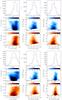 |
Fig. 9 Color–magnitude diagram and color distribution for all colors of the field l = 0.00, b = −1.00, same as Fig. 8. |
5.1. Extinction along different lines of sight
As an example of our results we discuss in more detail two specific lines of sight: the reference field (l, b) = (0.00, 1.00) and the field at (l, b) = (0.00, −1.00).
Figures 8 and 9 show the corresponding color–magnitude diagrams and color distribution for the observational data and the simulated data with the best-fitted final extinction in each filter. In addition to the general good agreement in the shape of the color–magnitude diagram and in the color distribution, we also emphasize that the number densities in the color–magnitude diagrams between the observations and the model agree very well. However, we notice some interesting features by comparing the color–magnitude diagrams of the model and the observations:
-
We clearly see in the [5.8] vs. Ks–[5.8] and especially in the [8.0] vs. Ks–[8.0] GLIMPSE-II diagram the AGB phase. The tip of the AGB is approximately slightly brighter than 8.0 mag at [8.0] . This phase is not reproduced by the model and needs to be improved.
-
In contrast to GLIMPSE II, the model predicts too many stars for VVV in all filters at the fainter end of the color–magnitude diagram. We suspect that the completeness limit of VVV is underestimated. Saito et al. (2012) analyzed for two VVV fields the completeness limit by using artificial sources. They found that the source detection efficiency reaches 50% for stars with 16.4 < Ks < 16.9 mag for tile b314 located at (l, b) = (352.21, −0.92). Our derived completeness limit is Ks = 14.9, which reaches the 75% completeness level according to Saito et al. (2012). A detailed analysis of the completeness limits of the VVV survey using artificial sources would be needed.
-
We notice that the model has produced a second branch in the J–Ks vs. Ks diagram at about Ks = 12.5 mag, which we do not find in the VVV data (see Fig. 9). This branch is related mainly to the Galactic disk K-giant population, which is clearly too prominent in the model. In contrast to the J–Ks and H–Ks color, the J–H color shows a large scatter in the temperature vs. color relation. This scatter is mainly due to the strong influence of J–H on metallicity and gravity (see also Bessell et al. 1989). We therefore decided to exclude the J–H color from our analysis.
Figure 10 to Fig. 13 show the change in interstellar extinction with distance in the different bands for four subfields. Different symbols stand for different data set: squares for VVV data and triangles for GLIMPSE-II data, while different colors denote the various filters. The errors of the derived distances and the extinction were calculated using the bootstrap method (Wall & Jenkins 2003). We re-sampled the original datasets of the observational and the model data 1000 times. The rms scatter gives the uncertainty of our results. Figure 14 shows a typical example. It shows the distributions of our results obtained for the 1000 samples obtained for one color bin (Step 3 in Sect. 4) for the GLIMPSE-II data in [3.6], left for the distance and right for the extinction. A Gaussian fit was made to the distributions, where the full-width-half maximum of the distribution gives the uncertainty in distance and extinction. This process is applied for each bin and each filter. The extinction changes along with the distance. As expected, it is higher for increasing distance. As seen in Fig. 10 to Fig. 13, the extinction becomes flatter beyond 7 kpc. As shown by Marshall et al. (2006), this is probably because inside the molecular ring the density of interstellar matter is lower than outside. It has also been shown that this region contains the dust lanes of the bar (Marshall et al. 2009), which can explain that at positive longitudes one can see an increase of the absorbing matter after this plateau, while it appears to be farther away at negative longitudes.
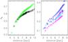 |
Fig. 10 Distance vs. extinction diagram for subfield l = 0.00, b = + 1.00. Left panel: green is AKs, H − Ks and black is AKs, J − Ks; right panel: blue is A [3.6] , K − [3.6] , violet A [4.5] , Ks − [4.5] , light blue A [5.8] , K − [5.8] , magenta A [8.0] , K − [8.0] . |
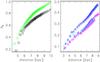 |
Fig. 11 Distance vs. extinction diagram for subfield l = 0.00, b = −1.00. The symbols are the same as in Fig. 10. |
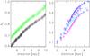 |
Fig. 12 Distance vs. extinction diagram for subfield l = 10.00, b = 1.00. The symbols are the same as in Fig. 10. |
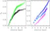 |
Fig. 13 Distance vs. extinction diagram for subfield l = 0.00, b = + 1.75. The symbols are the same as in Fig. 10. |
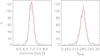 |
Fig. 14 Distribution of the distance (left) and the extinction (right) derived from 1000 samples with a bootstrap method. |
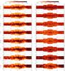 |
Fig. 15 3D extinction and error maps for AKs. The x-axis denotes the Galactic longitude and the y-axis the Galactic latitude. The units are in δAKs kpc-1. The map shows the weighted average extinction converted from the seven individual color excesses using the reddening law derived in Sect. 6. |
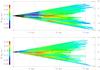 |
Fig. 16 Dust extinction in the Galactic plane for |b| < 0.25. The dotted lines correspond to distances of 5, 10, and 15 kpc. The Sun position is marked as X and the Galactic center as +. Indicated on the y-axis is the Galactic longitude. The upper panel shows our results and the lower one those from Marshall et al. (2006). |
As already mentioned in Sect. 2.3, the VVV data used here are only for Ks fainter than 12 mag. For this reason, the first bin of the VVV data is 4 kpc. The VVV data on the other hand go much deeper (d ~ 10−12 kpc). But 2MASS starts to be incomplete at 12 mag depending on the line of sight. Therefore, there is in general a very small overlap between 2MASS and VVV, which is also seen in the color–magnitude diagrams (see Figs. 8 and 9) where we miss the bright foreground branch of K giants in the VVV data that is clearly visible in GLIMPSE II. For the four [IRAC] bands we see very similar extinction vs. distance relations.
5.2. Three-dimensional extinction map
To visualize the distribution of extinction in 3D, we divided the extinction between subsequent bins by the distance between them, similar as in Marshall et al. (2006). The distance intervals are interpolated in bins of 1 kpc. All 3D maps using the six different color excesses i.e. E(J − Ks), E(H − Ks), E(K − [3.6] ), E(K − [4.5] ), E(K − [5.8] ), and E(K − [8.0] ), are presented in Appendix A. The units are in kpc-1. In addition we also show the error maps for each pair of filters. These errors are calculated using the bootstrap method. On average the errors are lowest between 4–8 kpc. We see a very similar picture of the dust distribution very concentrated to the Galactic plane in all maps. As expected, extinction becomes higher as the distance from the Sun increases.
We converted the seven color excesses to AKs using the extinction law derived in Sect. 6 separately. The extinction map of the weighted mean values is shown in Fig. 15. The maps are presented as extinction in Ks band and are also in units of kpc-1. To better visualize the dust extinction along the line of sight, Fig. 16 shows a view of our results (upper panel) together with that from Marshall et al. (2006) (lower panel) from the north Galactic pole toward the Galactic plane at |b| < 0.25 similar to Fig. 9 of Marshall et al. (2006). Our results show generally similar structures compared to Marshall et al. (2006). Except for l = 00 and l = −70 we notice a very smooth and featureless dust extinction beyond 6 kpc. Clearly visible in this comparison is also the much lower extinction until 6 kpc compared to Marshall et al. (2006), which we discuss in Sect. 5.3. The highest concentration of dust is around the central molecular zone, a giant molecular cloud complex with an asymmetric distribution of molecular gas (see e.g. Morris & Serabyn 1996). The dust extinction map shows a non-axisymmetric structure very similar to that observed in OH and CO. However, the spatial resolution of our map is not high enough to trace features like the 100 pc elliptical and twisted ring of cold dust discovered by Molinari et al. (2011).
The highest extincted regions are best traced by E(H − Ks) using the VVV data and E(Ks − [3.6] ) going up to AKs = 3.5 mag. Thanks to the high sensitivity of VVV, we are able to trace highly extincted regions in 3D (such as star-forming regions, molecular clouds, etc.) up to distances of 10 kpc.
Concerning the E(Ks − [8.0] ) map, we emphasize that at 8 μm PAHs become an important component of emission that weakens the stellar flux (see e.g. Cotera et al. 2006). We find systematically higher extinction due to the PAHs emission.
Figure 17 shows the comparison in the two-dimensional space between the color excess using E(J − Ks) and the E(H − Ks), E(Ks − [3.6] ), E(Ks − [4.5] ), E(Ks − [5.8] ), and E(Ks − [8.0] ) to check whether we introduced any systematic offsets between the different filter pairs. Points with bootstrapping errors larger than 1σ were excluded. In general we see a very good relation with a difference not larger than 0.1 mag. The dispersion is higher for the GLIMPSE II data, which is due to the larger photometric errors.
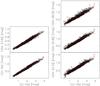 |
Fig. 17 Comparison of derived color excess values from J–Ks (VVV) to H–Ks (VVV), Ks–[3.6] (GLIMPSE-II), Ks–[4.5] (GLIMPSE-II), Ks–[5.8] (GLIMPSE-II), and Ks–[8.0] (GLIMPSE-II). |
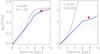 |
Fig. 18 3D extinction comparison with Marshall et al. (2006) and Drimmel et al. (2003), where the black solid line is for Drimmel et al. (2003), the black dashed line for Marshall et al. (2006), and the blue line is the result of our determination. The star symbols denote the calculated distance of the corresponding red-clump position of Gonzalez et al. (2012). |
5.3. Comparison with other 3D maps
We compared our results with those from Marshall et al. (2006) and Drimmel et al. (2003) for the extinction in the Ks band. Figure 18 shows the extinction v.s. distance diagram for two different fields, one located at (l, b) = (0.00, 1.00) and the other at extremely high extinction located at the Galactic center (l = 0.00, b = 0.00) compared to the dust model of Drimmel et al. (2003) and to Marshall et al. (2006).
We can see that they show the same trend as mentioned in Sect. 5.1. The black solid line is from Drimmel et al. (2003) and the dotted line from Marshall et al. (2006). To compare our results with those of Marshall et al. (2006), we converted their AKs values assuming the extinction coefficients of Nishiyama et al. (2009). Figure 18 shows that we obtain a similar AKs vs. distance relation for d > 6 kpc for our reference field (l, b) = (0, +1) while Marshall et al. predict a rather steep slope for d < 6 kpc. For the high-extinction field at (l, b) = (0, 0) there is quite a significant difference. We obtain a steeper slope and systematically higher extinction values for d > 4 kpc. We also added for comparison a data point of the 2D map of Gonzalez et al. (2012) that is marked as star symbol on the diagram. The distance was calculated by taking the difference of the dereddened mean magnitude of the red clump and the absolute magnitude of the red clump, which we assume to be MKs = −1.55 mag. Evidently the estimated distances from Gonzalez et al. (2012) agree remarkably well with our distances. Schödel et al. (2010) used adaptive optics observations of the central parsec of the Galactic center in the Ks band to map the extinction. They obtained a mean extinction value around Sagittarius A∗ of AKs = 2.46m with a distance to the Galactic center of R0 = 8.02 kpc, while Fritz et al. (2011) derived AKs = 2.42m. Our derived value of AKs = 2.34m is within the errors of the cited papers.
For low-extinction fields, our results agree with Marshall et al. (2006). Only for larger distances do we obtain slightly higher AKs values than Marshall et al. (2006). However, for the highly extincted fields such as the Galactic center (right panel of Fig. 18), we notice quite significant differences: While the extinction seems to flatten at a distance of about 6 kpc for Marshall et al. (2006), we notice a steady increase in extinction, reaching values of AKs = 2.5m compared to only AKs = 1.5m for Marshall et al. (2006). This low limit is due to the large incompleteness of 2MASS in this highly extincted region compared to the VVV. We emphasize that compared to Marshall et al. (2006) our distance steps shown here are much smaller and we therefore trace the derived distance-color relations better.
Thanks to its deeper photometry and higher spatial resolution, the VVV survey catalog has stars at larger distances than 2MASS. For a red clump star with MKs = −1.65m for example, a brightness at Ks = 12m, which is the reliable measurement by 2MASS toward crowded regions, means a distance of about 3.5 kpc with AKs = 1 mag, and 5.5 kpc if no extinction is applied. Since the Marshall results are derived based on the 2MASS data, there are difficulties in probing far and highly extincted regions. In contrast, at Ks = 15 mag the red clump star in the VVV survey can be detected at a distance of 13.4 kpc if AKs = 1 mag and 5.4 kpc if AKs = 3 mag. Considering the RGB and AGB stars that are mostly brighter than red clump stars, the VVV survey detected many stars at a distance farther than 5 kpc. This depth of the VVV makes the results at larger distance more solid. This also explains the systematically higher extinction we obtained for the Galactic center field at l = 0.0 and b = 0.0 (see Fig. 18) compared to Marshall et al. (2006).
Our results are clearly very different from those of Drimmel et al. (2003), in particular for the Galactic center region. The Drimmel model predicts much higher extinction than ours or Marshall’s. The dust model of Drimmel et al. (2003) strongly depends on the dust temperature. However, in the Galactic center region the gas pressure and temperature is higher than in the Galactic disk (see Serabyn & Morris 1996), which explains the large difference in the extinction values compared to Drimmel et al. (2003). Our map is not sensitive to dust temperature like theirs, but to the modeled K/M giant stellar population. Because our map is restricted to a spatial resolution of 15′ × 15′, small-scale variations such as seen, e.g., by Gosling et al. (2008) cannot be resolved.
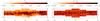 |
Fig. 19 2D extinction and error map for AKs integrated to a distance of 8 kpc. The map shows the weighted average extinction converted from the seven individual colors excesses using the reddening law derived in Sect. 6. The x-axis denotes the Galactic longitude and the y-axis the Galactic latitude. |
5.4. Two-dimensional extinction maps
We compared our extinction maps with the 2D-maps of Schultheis et al. (1999) and Gonzalez et al. (2012). While Schultheis et al. (1999) mainly used the RGB/AGB star population, Gonzalez et al. (2012) restricted themselves to the red clump stars to trace the extinction. To compare this with our results, we integrated our extinction map up to a distance to 8 kpc. The resulting 2D-maps of the combined AKs are shown in Fig. 19. The individual maps of the different color excesses are presented in Appendix B. They clearly show dust features very similar to those described in Schultheis et al. (1999) and Gonzalez et al. (2012). We clearly see the small-scale variation of the interstellar dust clouds concentrated toward the Galactic plane, which is not symmetric. In addition to the clear dust features of the central molecular zone,we also see a clear correlation between the high extinction and the number of detected infrared dark clouds based on molecular line observations (Jackson et al. 2008), especially at the region around (l, b) = (353.0, 0.0) with a strong concentration of young stellar objects.
For a more quantitative comparison we smoothed the Gonzalez et al. (2012) maps to the same spatial resolution as ours (15′ × 15′) and corrected for differences in the extinction law. Figure 20 shows the comparison. We see an excellent agreement between these maps with no systematic offset. For AKs > 1.5 mag the dispersion between our map and that of Schultheis et al. (1999) increases which is caused mainly by the limited sensitivity of the DENIS survey in the J- and Ks bands. In contrast, the dispersion compared to the VVV extinction is quite low, even for higher AK. We are therefore confident that our extinction determination is highly reliable.
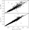 |
Fig. 20 Comparison of AKs with Schultheis et al. (1999) (top panel) and Gonzalez et al. (2012) (lower panel). |
Figure 21 shows that the intrinsic dispersion grows with increasing extinction. Lada et al. (1994) demonstrated that the form of the observed σdisp versus AV relation can be used to place constraints on the nature of the spatial distribution of extinction. However, photometric uncertainties as well as uncertainties in the extinction law dominate this relation. The dispersion in the VVV is much lower than for 2MASS because of its much smaller photometric errors. A higher spatial resolution would be needed to study this feature in more detail. The 2D maps of Gonzalez et al. (2012) have a 2′ × 2′ resolution resolution but their dispersion is dominated by the distribution of dust along the distance in that line of sight.
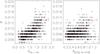 |
Fig. 21 Errors vs. the extinction diagram for the VVV (left panel) and 2MASS+GLIMPSE (right panel). The red solid line is an exponential fit. |
Figure 22 shows the total number of observed stars for each VVV subfield and the corresponding AKS. We clearly see that the number of stars gives an indication of the extinction, i.e., lower numbers mean higher extinction.
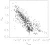 |
Fig. 22 Total number of stars for each VVV field as a function of AKS. |
6. Extinction coefficients
Because we determined the extinction maps using
E(λ − Ks), we can calculate the
extinction coefficients. For the extinction coefficients
Aλ/AKs,
we used here the values from Nishiyama et al. (2009)
as initial values. If λ is the wavelength we are going to derive and
α is the assumed wavelength, we can write
 (3)where
Aα/AKs
is the initial value for the assumed wavelength from Nishiyama et al. (2009).
E(λ − Ks)/(E(α − Ks))
is the color excess derived from the iteration of χ2 test (see
Sect. 4). Using Eq. (3), we derive the assumed wavelengths as J,
H, [3.6],[4.5],[5.8],[8.0] to calculate the extinction coefficients for
each subfield. The values we adopted are taken from Nishiyama et al. (2009) because the line of sight study is taken toward the
Galactic center. However, considering the variation of the extinction law that is suggested
by several studies, using a unique value
of Aα/AKs
could introduce some errors.
(3)where
Aα/AKs
is the initial value for the assumed wavelength from Nishiyama et al. (2009).
E(λ − Ks)/(E(α − Ks))
is the color excess derived from the iteration of χ2 test (see
Sect. 4). Using Eq. (3), we derive the assumed wavelengths as J,
H, [3.6],[4.5],[5.8],[8.0] to calculate the extinction coefficients for
each subfield. The values we adopted are taken from Nishiyama et al. (2009) because the line of sight study is taken toward the
Galactic center. However, considering the variation of the extinction law that is suggested
by several studies, using a unique value
of Aα/AKs
could introduce some errors.
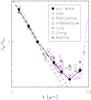 |
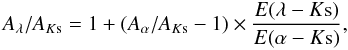
Fig. 23 Our derived interstellar extinction curve together with the comparison of different literature work. We used the mean extinction values over all fields. The red dashed line indicates a simple power law Aλ ∝ λ-1.75 from Draine (1989), the blue line the power law of Cardelli et al. (1989) with Aλ ∝ λ-1.61, and the green line depicts the power law of Fitzpatrick & Massa (2009) with Aλ ∝ λ-1.84. The dot-dashed line in magenta shows the extinction curve of Fritz et al. (2011) in the Galactic center. |
Extinction coefficients Aλ/AKs.
6.1. Mean extinction coefficients
Different choices of the assumed Aα/AKs would lead to different results for Aλ/AKs. We list our results in Table 3, varying the assumed extinction coefficient Aα/AKs. The mean extinction coefficients of all our fields are also listed in Table 3 and are compared to Gao et al. (2009), Indebetouw et al. (2005), and Nishiyama et al. (2009). The assumed values are noted in bold font in Table 3. Figure 23 shows the derived extinction curve. The black circles indicate our mean value (see Table 3). The red line indicates a simple power law Aλ ∝ λ-1.75 from Draine (1989), the blue line the power law of Cardelli et al. (1989) with Aλ ∝ λ-1.61, and the green line denotes the power law of Fitzpatrick & Massa (2009) with Aλ ∝ λ-1.84. Clearly these simple power laws cannot explain the flattening of the extinction curve between 3–8 μm. As shown by Gao et al. (2009) (see their Fig. 7), a larger mean dust grain size (e.g. 0.3 μm) would give a steeper extinction law (i.e., lower Aλ/AKs ratios) than that of the diffuse ISM where the mean dust size is 0.1 μm. Our derived extinction curve is very similar to that of Nishiyama et al. (2009). Interestingly, we find a lower A [5.8] /AKs value than Nishiyama et al. (2009). However, our value is within the errors close to the value of Nishiyama et al. (2009). Fritz et al. (2011) studied the near-IR and mid-IR extinction law toward Sgr A∗ using hydrogen emission lines. They found a power-law slope of alpha = −2.11 ± 0.06 shortward of 2.8 μm. This agree with our derived value of α = −2.175 and those found in the literature. Figure 23 shows that our derived extinction curve agrees remarkably well with that of Fritz et al. (2011) (indicated by the dot-dashed line) and confirms our low extinction value at [5.8]. As pointed out by Fritz et al. (2011), classical grain models (Li & Draine 2001; Weingartner & Draine 2001), using mainly silicate and graphite grains with different size distributions fails in reproducing the observed extinction law and especially the change of slope in the extinction law. Water ice features could be responsible for the slope change in the mid-IR. However, additional modeling is necessary.
The comparison shows that our mean values in the IRAC bands are comparable to those found in the literature. However, it depends on the assumed Aα/AKs. It can be seen from Table 3 that Aλ/AKs has lower values when Aα/AKs is bigger, which is a natural result from Eq. (3) because (Aα/AKs − 1) is negative for any wavelength longer than Ks. The values of AJ/AKs assumed or derived have a minimum of 2.56, a maximum of 2.89, and a mean of 2.70. In comparison, Gao et al. (2009) used AJ/AKs = 2.52.
 |
Fig. 24 Galactic longitude vs. Galactic latitude map of the A [3.6] /AKs extinction coefficient assuming AJ/AKs = 2.86 as long as longitudinal and latitudinal distribution of Aλ/AKs (λ equals to 3.6, 4.5, 5.8 and 8.0 μm). a) the distribution of Aλ/AKs as function of the Galactic longitude. Different colors denotes different wavelengths, the zero line stands for fixed AJ/AKs, and the black line indicates the data from Gao et al. (2009). b) The map of the A [3.6] /AKs extinction coefficient, the x-axis denotes the Galactic longitude, the y-axis the Galactic latitude. c) The same as a), but for the Galactic latitude. |
6.2. Variation of the extinction coefficients
The extinction coefficient may differ along different lines of sight. Gao et al. (2009) showed an interesting distribution of
extinction ratios as a function of Galactic longitude with 131 GLIMPSE fields. In this
work, we assumed the extinction
coefficients Aλ/AKs
for all subfields in our field. We took the median value of
the Aλ/AKs
in each bin of longitude or latitude. To see the variation clearly, we present here the
relative value ( ). Figure 24b shows a 2D map of
A [3.6] /AKs
assuming AJ/AKs = 2.86,
and Fig. 24a, c show the variation of the extinction
coefficients (i.e.,
A [3.6] /AKs,A [4.5] /AKs,A [5.8] /AKs,
and A [8.0] /AKs)
as a function of Galactic longitude (Fig. 24a) and
latitude (Fig. 24c). Overplotted in Fig. 24a are also the values from Gao et al. (2009). These authors used binsizes larger (1 degree) than
ours. We notice a similar behavior in all [IRAC] bands in the variation of the extinction
coefficient along the Galactic longitude, which follows the extinction curve variation of
Gao et al. (2009). While this variation is quite
small, we see a surprisingly strong peak visible toward the Galactic plane, indicating a
strong variation with Galactic latitude (see Fig. 24b). This variation seems to be stronger for longer wavelengths except
for 8.0 μm, where the amplitude becomes small again. This might be
related to the 9.7 μm silicate absorption feature (Gao et al. 2009). Figure 24
indicates that the extinction curve becomes flatter in the mid-IR, approaching the
Galactic center region. A detailed comparison with interstellar dust models is needed to
explain this feature, but this is beyond the scope of this paper.
). Figure 24b shows a 2D map of
A [3.6] /AKs
assuming AJ/AKs = 2.86,
and Fig. 24a, c show the variation of the extinction
coefficients (i.e.,
A [3.6] /AKs,A [4.5] /AKs,A [5.8] /AKs,
and A [8.0] /AKs)
as a function of Galactic longitude (Fig. 24a) and
latitude (Fig. 24c). Overplotted in Fig. 24a are also the values from Gao et al. (2009). These authors used binsizes larger (1 degree) than
ours. We notice a similar behavior in all [IRAC] bands in the variation of the extinction
coefficient along the Galactic longitude, which follows the extinction curve variation of
Gao et al. (2009). While this variation is quite
small, we see a surprisingly strong peak visible toward the Galactic plane, indicating a
strong variation with Galactic latitude (see Fig. 24b). This variation seems to be stronger for longer wavelengths except
for 8.0 μm, where the amplitude becomes small again. This might be
related to the 9.7 μm silicate absorption feature (Gao et al. 2009). Figure 24
indicates that the extinction curve becomes flatter in the mid-IR, approaching the
Galactic center region. A detailed comparison with interstellar dust models is needed to
explain this feature, but this is beyond the scope of this paper.
7. Conclusion
Using an improved version of the Besançon model, we presented here 3D extinction maps in the J, H, Ks, [3.6], [4.5], [5.8], and [8.0] bands using GLIMPSE II and VVV data. All extinction maps are available online at CDS (Tables 1 and 2), or through the BEAMER webpage2. We derived new temperature−color relations for M-giants, which match the observed color–magnitude diagrams better.
We presented 3D maps from 1.25 μm until 8 μm. Owing to the high sensitivity of the VVV data, we were able to trace high extinction until 10 kpc. Our maps integrated along the line of sight up to 8 kpc show an excellent agreement with the 2D-maps from Schultheis et al. (2009) and Gonzalez et al. (2012). These maps show the same dust features and consistent AKs values.
Using the initial value from Nishiyama et al. (2009), we derived the mean extinction coefficient of our field in the seven bands AJ/AKs = 2.70 ± 0.13, AH/AKs = 1.63 ± 0.03, A [3.6] /AKs = 0.53 ± 0.02, A [4.5] /AKs = 0.40 ± 0.02, A [5.8] /AKs = 0.32 ± 0.04, and A [8.0] /AKs = 0.42 ± 0.05. The variation of the coefficients indicates that the wavelength dependence of interstellar extinction in the mid-IR varies for different lines of sight, which means that there is no universal IR extinction law. This also agree with the study of Gao et al. (2009).
Online material
Appendix A: 3D reddening maps
 |
Fig. A.1 3D reddening and error maps for J–Ks VVV. The x-axis denotes the Galactic longitude and the y-axis the Galactic latitude. The units are in δE(J − Ks) kpc-1. |
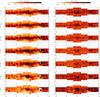 |
Fig. A.2 3D reddening and error maps for E(H–Ks) VVV. |
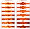 |
Fig. A.3 3D reddening and error maps for E(Ks–[3.6]). |
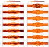 |
Fig. A.4 3D reddening and error maps for E(Ks–[4.5]). |
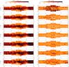 |
Fig. A.5 3D reddening and error maps for E(Ks–[5.8]). |
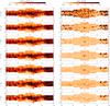 |
Fig. A.6 3D reddening and error maps for E(Ks–[8.0]). |
Appendix B: 2D reddening maps
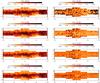 |
Fig. B.1 2D reddening and error map for E(Ks–[3.6]), E(Ks–[4.5]), E(Ks–[5.8], and E(K–[8.0]) integrated to 8 kpc distance. |
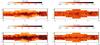 |
Fig. B.2 2D reddening and error map for E(J–Ks), E(H–Ks) in the VVV bands integrated to 8 kpc distance. |
Acknowledgments
We want to thank the referee for his/her fruitful comments. We gratefully acknowledge use of data from the ESO Public Survey program ID 179.B-2002 taken with the VISTA telescope, data products from the Cambridge Astronomical Survey Unit and funding from the FONDAP center for Astrophysics 15010003, the BASAL CATA center for Astrophysics and Associated Technologies PFB-06, the MILENIO Milky Way Millennium Nucleus from the Ministry of Economy ICM grant P07-021-F, and the FONDECYT the Proyecto FONDECYT Regular No. 1090213. We are grateful to the GLIMPSE-II project for providing access to the data. B.Q.C. was supported by a scholarship of the China Scholarship Council (CSC).
References
- Babusiaux, C., Gómez, A., Hill, V., et al. 2010, A&A, 519, A77 [NASA ADS] [CrossRef] [EDP Sciences] [Google Scholar]
- Bensby, T., Adén, D., Meléndez, J., et al. 2011, A&A, 533, A134 [NASA ADS] [CrossRef] [EDP Sciences] [Google Scholar]
- Bertelli, G., Bressan, A., Chiosi, C., Fagotto, F., & Nasi, E. 1994, A&AS, 106, 275 [NASA ADS] [Google Scholar]
- Bessell, M. S., Brett, J. M., Wood, P. R., & Scholz, M. 1989, A&AS, 77, 1 [NASA ADS] [Google Scholar]
- Cardelli, J. A., Clayton, G. C., & Mathis, J. S. 1989, ApJ, 345, 245 [NASA ADS] [CrossRef] [Google Scholar]
- Churchwell, E., Babler, B. L., Meade, M. R., et al. 2009, PASP, 121, 213 [NASA ADS] [CrossRef] [Google Scholar]
- Cotera, A., Stolovy, S., Ramirez, S., et al. 2006, J. Phys. Conf. Ser., 54, 183 [NASA ADS] [CrossRef] [Google Scholar]
- Draine, B. T. 1989, in Infrared Spectroscopy in Astronomy, ed. E. Böhm-Vitense, ESA SP, 290, 93 [Google Scholar]
- Drimmel, R., Cabrera-Lavers, A., & López-Corredoira, M. 2003, A&A, 409, 205 [NASA ADS] [CrossRef] [EDP Sciences] [Google Scholar]
- Dutra, C. M., Santiago, B. X., Bica, E. L. D., & Barbuy, B. 2003, MNRAS, 338, 253 [NASA ADS] [CrossRef] [Google Scholar]
- Fazio, G. G., Hora, J. L., Allen, L. E., et al. 2004, ApJS, 154, 10 [NASA ADS] [CrossRef] [Google Scholar]
- Fitzpatrick, E. L., & Massa, D. 2009, ApJ, 699, 1209 [NASA ADS] [CrossRef] [Google Scholar]
- Fritz, T. K., Gillessen, S., Dodds-Eden, K., et al. 2011, ApJ, 737, 73 [NASA ADS] [CrossRef] [Google Scholar]
- Gao, J., Jiang, B. W., & Li, A. 2009, ApJ, 707, 89 [NASA ADS] [CrossRef] [Google Scholar]
- Girardi, L., Williams, B. F., Gilbert, K. M., et al. 2010, ApJ, 724, 1030 [NASA ADS] [CrossRef] [Google Scholar]
- Gonzalez, O. A., Rejkuba, M., Zoccali, M., Valenti, E., & Minniti, D. 2011, A&A, 534, A3 [NASA ADS] [CrossRef] [EDP Sciences] [Google Scholar]
- Gonzalez, O. A., Rejkuba, M., Zoccali, M., et al. 2012, A&A, 543, A13 [NASA ADS] [CrossRef] [EDP Sciences] [Google Scholar]
- Gosling, A. J., Blundell, K. M., Bandyopadhyay, R. M., & Lucas, P. 2008, in A Population Explosion: The Nature & Evolution of X-ray Binaries in Diverse Environments, eds. R. M. Bandyopadhyay, S. Wachter, D. Gelino, & C. R. Gelino, AIP Conf. Ser., 1010, 168 [Google Scholar]
- Houdashelt, M. L., Bell, R. A., Sweigart, A. V., & Wing, R. F. 2000, AJ, 119, 1424 [NASA ADS] [CrossRef] [Google Scholar]
- Indebetouw, R., Mathis, J. S., Babler, B. L., et al. 2005, ApJ, 619, 931 [NASA ADS] [CrossRef] [Google Scholar]
- Jackson, J. M., Finn, S. C., Rathborne, J. M., Chambers, E. T., & Simon, R. 2008, ApJ, 680, 349 [NASA ADS] [CrossRef] [Google Scholar]
- Jiang, B. W., Gao, J., Omont, A., Schuller, F., & Simon, G. 2006, A&A, 446, 551 [NASA ADS] [CrossRef] [EDP Sciences] [Google Scholar]
- Lada, C. J., Lada, E. A., Clemens, D. P., & Bally, J. 1994, ApJ, 429, 694 [NASA ADS] [CrossRef] [Google Scholar]
- Lejeune, T., Cuisinier, F., & Buser, R. 1997, A&AS, 125, 229 [NASA ADS] [CrossRef] [EDP Sciences] [Google Scholar]
- Lejeune, T., Cuisinier, F., & Buser, R. 1998, A&AS, 130, 65 [NASA ADS] [CrossRef] [EDP Sciences] [Google Scholar]
- Li, A., & Draine, B. T. 2001, ApJ, 554, 778 [Google Scholar]
- Marigo, P., Girardi, L., Bressan, A., et al. 2008, A&A, 482, 883 [NASA ADS] [CrossRef] [EDP Sciences] [Google Scholar]
- Marshall, D. J., Robin, A. C., Reylé, C., Schultheis, M., & Picaud, S. 2006, A&A, 453, 635 [NASA ADS] [CrossRef] [EDP Sciences] [Google Scholar]
- Marshall, D. J., Fux, R., Robin, A. C., & Reylé, C. 2009, in The Evolving ISM in the Milky Way and Nearby Galaxies [Google Scholar]
- Minniti, D., Lucas, P. W., Emerson, J. P., et al. 2010, New A, 15, 433 [NASA ADS] [CrossRef] [Google Scholar]
- Molinari, S., Bally, J., Noriega-Crespo, A., et al. 2011, ApJ, 735, L33 [NASA ADS] [CrossRef] [Google Scholar]
- Morris, M., & Serabyn, E. 1996, ARA&A, 34, 645 [NASA ADS] [CrossRef] [Google Scholar]
- Nidever, D. L., Zasowski, G., & Majewski, S. R. 2012, ApJS, 201, 35 [NASA ADS] [CrossRef] [Google Scholar]
- Nishiyama, S., Tamura, M., Hatano, H., et al. 2009, ApJ, 696, 1407 [NASA ADS] [CrossRef] [Google Scholar]
- Ojha, D. K., Omont, A., Schuller, F., et al. 2003, A&A, 403, 141 [NASA ADS] [CrossRef] [EDP Sciences] [Google Scholar]
- Omont, A., Ganesh, S., Alard, C., et al. 1999, A&A, 348, 755 [NASA ADS] [Google Scholar]
- Omont, A., Gilmore, G. F., Alard, C., et al. 2003, A&A, 403, 975 [NASA ADS] [CrossRef] [EDP Sciences] [Google Scholar]
- Press, W. H., Teukolsky, S. A., Vetterling, W. T., & Flannery, B. P. 1992, Numerical recipes in FORTRAN. The art of scientific computing (Cambridge University Press) [Google Scholar]
- Ramírez, S. V., Arendt, R. G., Sellgren, K., et al. 2008, ApJS, 175, 147 [NASA ADS] [CrossRef] [Google Scholar]
- Robin, A. C., Reylé, C., Derrière, S., & Picaud, S. 2003, A&A, 409, 523 [NASA ADS] [CrossRef] [EDP Sciences] [Google Scholar]
- Robin, A. C., Marshall, D. J., Schultheis, M., & Reylé, C. 2012, A&A, 538, A106 [NASA ADS] [CrossRef] [EDP Sciences] [Google Scholar]
- Saito, R. K., Hempel, M., Minniti, D., et al. 2012, A&A, 537, A107 [NASA ADS] [CrossRef] [EDP Sciences] [Google Scholar]
- Schödel, R., Najarro, F., Muzic, K., & Eckart, A. 2010, A&A, 511, A18 [NASA ADS] [CrossRef] [EDP Sciences] [Google Scholar]
- Schultheis, M., Ganesh, S., Simon, G., et al. 1999, A&A, 349, L69 [NASA ADS] [Google Scholar]
- Schultheis, M., Sellgren, K., Ramírez, S., et al. 2009, A&A, 495, 157 [NASA ADS] [CrossRef] [EDP Sciences] [Google Scholar]
- Serabyn, E., & Morris, M. 1996, Nature, 382, 602 [NASA ADS] [CrossRef] [Google Scholar]
- Taylor, M. B. 2006, in Astronomical Data Analysis Software and Systems XV, eds. C. Gabriel, C. Arviset, D. Ponz, & S. Enrique, ASP Conf. Ser., 351, 666 [Google Scholar]
- Uttenthaler, S., Stute, M., Sahai, R., et al. 2010, A&A, 517, A44 [NASA ADS] [CrossRef] [EDP Sciences] [Google Scholar]
- Uttenthaler, S., Blommaert, J. A. D. L., Lebzelter, T., et al. 2012, Assembling the Puzzle of the Milky Way, Le Grand-Bornand, France, eds. C. Reylé, A. Robin, & M. Schultheis, EPJ Web Conf., 19, 6009 [Google Scholar]
- Wall, J. V., & Jenkins, C. R. 2003, Practical Statistics for Astronomers, eds. R. Ellis, J. Huchra, S. Kahn, G. Rieke, & P. B. Stetson [Google Scholar]
- Weingartner, J. C., & Draine, B. T. 2001, ApJ, 548, 296 [NASA ADS] [CrossRef] [Google Scholar]
- Werner, M. W., Roellig, T. L., Low, F. J., et al. 2004, ApJS, 154, 1 [Google Scholar]
- Zasowski, G., Majewski, S. R., Indebetouw, R., et al. 2009, ApJ, 707, 510 [NASA ADS] [CrossRef] [Google Scholar]
- Zoccali, M., Renzini, A., Ortolani, S., et al. 2003, A&A, 399, 931 [NASA ADS] [CrossRef] [EDP Sciences] [Google Scholar]
- Zoccali, M., Hill, V., Lecureur, A., et al. 2008, A&A, 486, 177 [NASA ADS] [CrossRef] [EDP Sciences] [Google Scholar]
All Tables
Extinction as a function of Galactic longitude, latitude, and distance based on VVV data.
Extinction as a function of Galactic longitude, latitude, and distance based on GLIMPSE-II data.
All Figures
|
Fig. 1 Star counts of GLIMPSE-II data of two example fields for the 2MASS bands and IRAC bands. Each field is 15′ × 15′. |
| In the text | |
|
Fig. 2 Star counts of VVV-survey data of two example fields for the 2MASS bands. Each field is 15′ × 15′. |
| In the text | |
|
Fig. 3 Comparison of the the simulated color–magnitude diagrams using the old Teff vs. color relation (left) compared to the new one (right) for the reference field (l = 0.00 and b = 1.00). The color bar indicates the number of the stars. |
| In the text | |
|
Fig. 4 a): log Teff vs. log g grid in the Besançon model. Black triangles indicate the coverage of the Besançon model (Robin et al. 2003) while red stars show the new extended grid. b): J–Ks vs. Teff relation. Black triangles show the old relation and red crosses the new one. The blue symbols is the relation for M giants from Houdashelt et al. (2000). c): Similar as b) but for K–[4.5] vs. Teff. |
| In the text | |
|
Fig. 5 Comparison of the Ks–[4.5] vs. [4.5] diagram of Baade window (left panel) with the old (middle panel) and the new temperature vs. color relation (left panel). The data are from Uttenthaler et al. (2010). The color bar indicates the number of the stars. |
| In the text | |
|
Fig. 6 Calculation process for the extinction of the example subfield (l, b) of (0.0, +1.0). From upper left to lower right, they are a) the errors of [3.6] vs. the [3.6] diagram, b) the color Ks–[3.6] vs. distance diagram, c) the extinction at [3.6] vs. the distance diagram where we show the first initial guess of extinction after the first iteration (black) and the final iteration after 20 loops, (red) and d) the color Ks–[3.6] distribution of the data compared to the first guess iteration (black) and the final one (red). |
| In the text | |
|
Fig. 7 Test of our method. The red line is the artificial extinction with clouds. The black crosses show our derived extinction values. The left panel is of field (l, b) = (0.00, +1.00) and the right of field (l, b) = (5.00, 0.00). |
| In the text | |
|
Fig. 8 Color–magnitude diagram and color distribution for all colors of the field l = 0.00, b = 1.00. The lower panel shows the observed color–magnitude diagram, the middle panel the synthetic color–magnitude diagram with the best-fitted extinction, and the upper panel shows the histograms in the color distribution. The red color scale (lower panel) shows the observations (noted as “VVV or GLIMPSE” in the title of the inner color bar) while the blue color scale shows the simulated data (noted as “model”). The dashed lines show the completeness limit. The color bar inside the color–magnitude diagram shows the number of stars of each corresponding dataset. |
| In the text | |
|
Fig. 9 Color–magnitude diagram and color distribution for all colors of the field l = 0.00, b = −1.00, same as Fig. 8. |
| In the text | |
|
Fig. 10 Distance vs. extinction diagram for subfield l = 0.00, b = + 1.00. Left panel: green is AKs, H − Ks and black is AKs, J − Ks; right panel: blue is A [3.6] , K − [3.6] , violet A [4.5] , Ks − [4.5] , light blue A [5.8] , K − [5.8] , magenta A [8.0] , K − [8.0] . |
| In the text | |
|
Fig. 11 Distance vs. extinction diagram for subfield l = 0.00, b = −1.00. The symbols are the same as in Fig. 10. |
| In the text | |
|
Fig. 12 Distance vs. extinction diagram for subfield l = 10.00, b = 1.00. The symbols are the same as in Fig. 10. |
| In the text | |
|
Fig. 13 Distance vs. extinction diagram for subfield l = 0.00, b = + 1.75. The symbols are the same as in Fig. 10. |
| In the text | |
|
Fig. 14 Distribution of the distance (left) and the extinction (right) derived from 1000 samples with a bootstrap method. |
| In the text | |
|
Fig. 15 3D extinction and error maps for AKs. The x-axis denotes the Galactic longitude and the y-axis the Galactic latitude. The units are in δAKs kpc-1. The map shows the weighted average extinction converted from the seven individual color excesses using the reddening law derived in Sect. 6. |
| In the text | |
|
Fig. 16 Dust extinction in the Galactic plane for |b| < 0.25. The dotted lines correspond to distances of 5, 10, and 15 kpc. The Sun position is marked as X and the Galactic center as +. Indicated on the y-axis is the Galactic longitude. The upper panel shows our results and the lower one those from Marshall et al. (2006). |
| In the text | |
|
Fig. 17 Comparison of derived color excess values from J–Ks (VVV) to H–Ks (VVV), Ks–[3.6] (GLIMPSE-II), Ks–[4.5] (GLIMPSE-II), Ks–[5.8] (GLIMPSE-II), and Ks–[8.0] (GLIMPSE-II). |
| In the text | |
|
Fig. 18 3D extinction comparison with Marshall et al. (2006) and Drimmel et al. (2003), where the black solid line is for Drimmel et al. (2003), the black dashed line for Marshall et al. (2006), and the blue line is the result of our determination. The star symbols denote the calculated distance of the corresponding red-clump position of Gonzalez et al. (2012). |
| In the text | |
|
Fig. 19 2D extinction and error map for AKs integrated to a distance of 8 kpc. The map shows the weighted average extinction converted from the seven individual colors excesses using the reddening law derived in Sect. 6. The x-axis denotes the Galactic longitude and the y-axis the Galactic latitude. |
| In the text | |
|
Fig. 20 Comparison of AKs with Schultheis et al. (1999) (top panel) and Gonzalez et al. (2012) (lower panel). |
| In the text | |
|
Fig. 21 Errors vs. the extinction diagram for the VVV (left panel) and 2MASS+GLIMPSE (right panel). The red solid line is an exponential fit. |
| In the text | |
|
Fig. 22 Total number of stars for each VVV field as a function of AKS. |
| In the text | |
|
Fig. 23 Our derived interstellar extinction curve together with the comparison of different literature work. We used the mean extinction values over all fields. The red dashed line indicates a simple power law Aλ ∝ λ-1.75 from Draine (1989), the blue line the power law of Cardelli et al. (1989) with Aλ ∝ λ-1.61, and the green line depicts the power law of Fitzpatrick & Massa (2009) with Aλ ∝ λ-1.84. The dot-dashed line in magenta shows the extinction curve of Fritz et al. (2011) in the Galactic center. |
| In the text | |
|
Fig. 24 Galactic longitude vs. Galactic latitude map of the A [3.6] /AKs extinction coefficient assuming AJ/AKs = 2.86 as long as longitudinal and latitudinal distribution of Aλ/AKs (λ equals to 3.6, 4.5, 5.8 and 8.0 μm). a) the distribution of Aλ/AKs as function of the Galactic longitude. Different colors denotes different wavelengths, the zero line stands for fixed AJ/AKs, and the black line indicates the data from Gao et al. (2009). b) The map of the A [3.6] /AKs extinction coefficient, the x-axis denotes the Galactic longitude, the y-axis the Galactic latitude. c) The same as a), but for the Galactic latitude. |
| In the text | |
|
Fig. A.1 3D reddening and error maps for J–Ks VVV. The x-axis denotes the Galactic longitude and the y-axis the Galactic latitude. The units are in δE(J − Ks) kpc-1. |
| In the text | |
|
Fig. A.2 3D reddening and error maps for E(H–Ks) VVV. |
| In the text | |
|
Fig. A.3 3D reddening and error maps for E(Ks–[3.6]). |
| In the text | |
|
Fig. A.4 3D reddening and error maps for E(Ks–[4.5]). |
| In the text | |
|
Fig. A.5 3D reddening and error maps for E(Ks–[5.8]). |
| In the text | |
|
Fig. A.6 3D reddening and error maps for E(Ks–[8.0]). |
| In the text | |
|
Fig. B.1 2D reddening and error map for E(Ks–[3.6]), E(Ks–[4.5]), E(Ks–[5.8], and E(K–[8.0]) integrated to 8 kpc distance. |
| In the text | |
|
Fig. B.2 2D reddening and error map for E(J–Ks), E(H–Ks) in the VVV bands integrated to 8 kpc distance. |
| In the text | |
Current usage metrics show cumulative count of Article Views (full-text article views including HTML views, PDF and ePub downloads, according to the available data) and Abstracts Views on Vision4Press platform.
Data correspond to usage on the plateform after 2015. The current usage metrics is available 48-96 hours after online publication and is updated daily on week days.
Initial download of the metrics may take a while.