| Issue |
A&A
Volume 550, February 2013
|
|
|---|---|---|
| Article Number | A50 | |
| Number of page(s) | 14 | |
| Section | Interstellar and circumstellar matter | |
| DOI | https://doi.org/10.1051/0004-6361/201219423 | |
| Published online | 24 January 2013 | |
Ionisation impact of high-mass stars on interstellar filaments
A Herschel study of the RCW 36 bipolar nebula in Vela C ⋆,⋆⋆
1
Laboratoire AIM Paris-Saclay, CEA/IRFU-CNRS/INSU-Université Paris Diderot,
CEA Saclay,
91191
Gif-sur-Yvette Cedex,
France
e-mail: This email address is being protected from spambots. You need JavaScript enabled to view it.
2
Departamento de Astronomía, Universidad de Chile, Camino El
Observatorio 1515, Las Condes,
Santiago, 36- D
Casilla, Chile
3
The Rutherford Appleton Laboratory, Chilton, Didcot, OX11
0QX, UK
4
Department of Physics and Astronomy, The Open
University, Milton
Keynes, UK
5
School of Physics, University of New South Wales,
Sydney,
2052
NSW,
Australia
6
Laboratoire d’Astrophysique de Marseille, UMR 6110, CNRS –
Université de Provence, 38 rue F.
Joliot-Curie, 13388
Marseille,
France
7
National Research Council of Canada, 5071 West Saanich Road,
Victoria, V9E 2E7 BC,
Canada
8
IAPS − Instituto di Astrofisica e Planetologia Spaziali,
via Fosso del Cavaliere
100, 00133
Roma,
Italy
9
INAF − Osservatorio Astronomico di Roma, via Frascati 33,
00040
Monte Porzio Catone,
Italy
10 Jeremiah Horrocks Institute, University of Central
Lancashire, PR1 2HE, UK
Received:
16
April
2012
Accepted:
30
November
2012
Abstract
Context. Ionising stars reshape their original molecular cloud and impact star formation, leading to spectacular morphologies such as bipolar nebulae around H ii regions. Molecular clouds are structured in filaments where stars principally form, as revealed by the Herschel space observatory. The prominent southern hemisphere H ii region, RCW 36, is one of these bipolar nebulae.
Aims. We study the physical connection between the filamentary structures of the Vela C molecular cloud and the bipolar morphology of RCW 36, providing an in-depth view of the interplay occurring between ionisation and interstellar structures (bright-rims and pillars) around an H ii region.
Methods. We have compared Herschel observations in five far-infrared and submillimetre filters with the PACS and SPIRE imagers, to dedicated numerical simulations and molecular line mapping.
Results. Our results suggest that the RCW 36 bipolar morphology is a natural evolution of its filamentary beginnings under the impact of ionisation.
Conclusions. Such results demonstrate that, filamentary structures can be the location of very dynamical phenomena inducing the formation of dense clumps at the edge of H ii regions. Moreover, these results could apply to better understanding the bipolar nebulae as a consequence of the expansion of an H ii region within a molecular ridge or an interstellar filament.
Key words: ISM: individual objects: RCW 36 / ISM: individual objects: Vela C / ISM: structure / stars: massive / hydrodynamics / HII regions
Herschel is an ESA space observatory with science instruments provided by European-led Principal Investigator consortia and with important participation from NASA.
Appendices are available in electronic form at http://www.aanda.org
© ESO, 2013
1. Introduction
Ionising stars play a likely significant role in reshaping the molecular cloud and triggering star formation (e.g. Deharveng et al. 2010; Zavagno et al. 2010; Purcell et al. 2009; Minier et al. 2009). However, the actual impact of high-mass star radiation remains a debated scientific controversy in the literature (e.g. Hill et al. 2012; Schneider et al. 2012; Dale & Bonnell 2012; Tremblin et al. 2012a; Thompson et al. 2012; Flagey et al. 2011).
Among the molecular clouds with embedded ionising stars, many exhibit a spectacular, bipolar morphology. It consists of an H ii region and its cavity of ionised gas surrounded by molecular gas, a star cluster inside, and a dust lane that crosses the cavity and sometimes partly hides the ionising stars. S 106 (Bally et al. 1998), IRS16/Vela D (Strafella et al. 2010), NGC 3576 (Purcell et al. 2009), NGC 2024 (Mezger et al. 1992), S88 (White & Fridlung 1992) and S 201 (Mampaso et al. 1987), for instance, are among this type of H ii regions, and these could be referred as being hourglass-shaped nebulae, bipolar nebulae, or bi-lobed appearance nebulae (e.g. Staude & Elsässer 1994). In this paper, we investigate a possible connection between the actual morphology of these nebulae and the basic structures of the parent molecular clouds in light of recent Herschel observations of interstellar filamentary structures (André et al. 2010; Molinari et al. 2010; Hill et al. 2011). Can the interstellar features observed with Herschel teach us anything about the process turning a molecular cloud into a bipolar nebula?
RCW 36, at a distance of 700 pc from the Sun (Murphy & May 1991), is one hourglass-shaped environment (see Fig. 1). At the centre, an embedded cluster, 2–3 Myr old, has 350 members with the most massive star being a type O8 or O9 (Baba et al. 2004). The cluster extends over a radius of 0.5 pc, with a stellar surface number density of 3000 stars pc-2 within the central 0.1 pc. FIR emission and radio continuum emission are reported to be consistent with the presence of an H ii region (Verma et al. 1994). Massive stars lie at the centre of the cluster, while low mass stars and near-infrared (NIR) excess sources spread all over the H ii region (Baba et al. 2004). The massive stars have probably inflated the G265.151+1.454 H ii region (Caswell & Haynes 1987) that is responsible for the Hα emission originally observed by Rodger et al. (1960).
Looking at larger scales, RCW 36 is located within the Vela C molecular cloud that consists of an apparent network of filaments (Hill et al. 2011). Such filaments are star formation sites. Herschel observations of low-mass star-forming molecular clouds (e.g. Arzoumanian et al. 2011) show that stars form in supercritical filaments while Schneider et al. (2012) propose that massive star cluster-formation sites coincide with filament network junctions. Among the networks of filaments in Vela C, there is a more prominent and elongated interstellar dust structure of ~10 pc in length that was named the Centre-Ridge by Hill et al. It encompasses RCW 36, which is at its Southern end (Fig. 1).
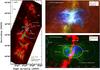 |
Fig. 1 a) Column density map of Vela C derived from Herschel observations at 160, 250, 350 and 500 μm with a resolution of 36″ (see Hill et al. 2011). The peak column density is ~1023 cm-2, although the column density range on this image is 2 × 10²¹–5 × 1022 cm-2 to emphasize both the high density filamentary structure and the more diffuse dust around. The “low density areas” are minima at a few 1021 cm-2 on the East and West sides of the H ii region. The RCW 36 area is indicated by a dashed box. White contours represent the radio continuum emission at 5 GHz. b) Zoom on the RCW 36 bipolar nebula as seen by Herschel at 70, 160 and 250 μm (in blue, green, red, respectively). c) Three-colour image of RCW 36 showing areas with column density from 2 × 10²¹ to 5 × 1022 cm-2 (red), temperature from 14 to 40 K (green) and Hα (blue). Hα emission is within a white ellipse, with a major axis oriented East-West. The column density exhibits a ring-like structure (white dashed-dotted ellipse), that is part of the Centre-Ridge. The hourglass or bipolar shape is suggested with a bi-lobed curve shown in blue. |
In this work, we focus on the interstellar environment of RCW 36 and analyse its morphology in relationship with the overall filamentary structure of Vela C. We investigate a possible scenario for which the ionising UV radiation from the star cluster is the main physical phenomenon that reshapes the Centre-Ridge as seen in the column density map, and creates a bipolar ionised nebula. In light of dedicated numerical hydrodynamic simulations based on work by Tremblin et al. (2012a), we finally explore the physical mechanisms that lead to the formation of bright rims and pillars-like structures1 as well as the triggered formation of dense star-forming clumps at the borders of the H ii region.
2. Herschel observations and complementary data
Vela C was observed on 2010, May 18 by Hill et al. (2011) as part of the HOBYS key programme (Motte et al. 2010) with the Herschel space observatory (Pilbratt et al. 2010). The parallel-scan mode of Herschel was used with PACS at 70 and 160 μm (5 and 12″ resolution; Poglitsch et al. 2010) and SPIRE at 250, 350, 500 μm (18″, 25″ and 36″ resolution; Griffin et al. 2010) with a scan speed of 20″s-1. A total area of 3 deg2 was mapped (see Hill et al. for details). In this paper, we focus on the RCW 36 region as part of the Vela C molecular cloud (see Fig. 1).
Complementary data at 450 μm for the RCW 36 area were obtained with the P-ArTéMiS bolometer camera (see André et al. 2008; Minier et al. 2009) on the APEX telescope during May 2009 as part of ESO programme 083.C-0996. This has allowed us to improve the angular resolution of the derived column density map in this area from 36″ in Hill et al. (2011) to 12″, by combining the Herschel 160 and 250 μm data with the P-ArTéMiS 450 μm data. To produce this column density map, a temperature map at the 18″ resolution of the SPIRE 250 μm observations was first derived based on the ratio of Herschel 160 and 250 μm data. The PACS 160 μm data (12″ resolution) and a slightly smoothed version of the P-ArTéMiS 450 μm data were then converted to a column density map at 12″ resolution, assuming optically thin dust emission at a fixed temperature given by the temperature map at each pixel and the same dust opacity law as in Hill et al. (2011) and Arzoumanian et al. (2011). This procedure is only approximate as it neglects any temperature variation on angular scales smaller than 18″ in the plane of the sky, as well as any temperature variation along the line of sight.
The dynamics of the region, such as the velocity information, is provided by the CS(1−0) line data mapped with the Mopra Telescope (CSIRO/CASS), as part of the continuing Vela C multi-molecular line mapping project at 3, 7 and 12 mm wavebands (PI: Cunningham, Maria). The RCW 36 region observations were carried out in 2009 and 2010 using the 8 GHz bandwidth UNSW-MOPS digital filterbank backend and the MMIC receiver. At 48 GHz the velocity resolution is 0.2 km s-1 and the FWHM beam size is 76″. The data were reduced using the Livedata and Gridzilla packages available from the CSIRO/CASS. Livedata performs a bandpass calibration for each row in the raster map using the preceding OFF scan and then fits a user-specified polynomial to the spectral baseline. Gridzilla grids the data according to user-specified weighting and beam parameter inputs. A first-order polynomial baseline fitting was used in the presented data and were weighted by the relevant Tsys measurements.
RCW 36 was also observed in May 2006 with Spitzer IRAC (PI: Tsujimoto, Masahiro). The data at 4.5 μm were retrieved from the Spitzer Heritage Archives. Complementary 2MASS K-band data provide the star cluster location. Finally to locate the H ii region and quantify its physical properties, archival Hα data were obtained from the SuperCOSMOS Sky Survey (Hambly et al. 2001), as well as a radio continuum map at 5 GHz was downloaded from the Parkes-MIT-NRAO (PMN) Surveys Web page (Condon et al. 1993).
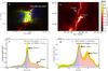 |
Fig. 2 a) Three-colour image of RCW 36 nebula (red: SPIRE 250 μm, green: PACS 70 μm, blue: Hα). The cross indicates the ionizing source. Each coloured circle indicates area for which CS spectra have been integrated as in Fig. 7. The ellipse highlights the ring of compressed gas. b) column density map around RCW 36. The DisPerSe skeleton is drawn in white and each part of the shocked layer is labeled front 1 and front 2. c) Profile of the front 1 traced by DisPerSe on a Herschel+P-ArTéMiS column density map at 12″ resolution. d) Profile of the front 2 traced by DisPerSe on a Herschel column density map at 36′′ resolution. The yellow shaded area represents the standard deviation of the profiles. The green- dashed curve is the Gaussian fit used to determinate the FWHM width. |
3. The RCW 36 bipolar nebula
3.1. Overall characteristics
The Vela C molecular cloud shows an elongated structure running approximately north-south, with a size of about 30 pc and mass of about 3 × 10⁴ M⊙, based on the Herschel column density map (Fig. 1a). RCW 36 is located close to the centre of Vela C. Focusing on the RCW 36 area, interstellar matter appears to have been cleared up to 1.5 pc away on each side of the star cluster where high-mass stars have already formed, revealing the dense filamentary structure: the Centre-Ridge (Fig. 1a). Hα emission is observed towards RCW 36 and traces an ionised gas shell of 1.8 pc in extent. The Hα emission falls within an ellipse with an East-West major axis (Fig. 1c). The corresponding radio continuum emission with a total flux of ~26 Jy at 4.8 GHz, derived from the PMN survey map, is consistent with an ionising photon flux of 6 × 1047 ph s-1 (i.e. a O9.5 star in Panagia 1973) and an electronic density of ~200 cm-3 assuming a temperature of 8000 K (see Martin-Hernandez et al. 2005, for detailed equations used for the calculation). For these physical parameters, the radius of a Strömgren sphere would be ~1 pc (Strömgren 1939).
The RCW 36 area is characterised by both an increase of column density by a factor of 10 inside the densest part of the Centre-Ridge with respect to a mean column density of ~3 × 1022 cm-2, and a decrease of the column density for up to 1.5 pc on each side of the ridge by a factor of 10 with respect to the mean density (the “low density” − a few 1021 cm-2 areas seen in Fig. 1a). These two areas of much lower column density terminate the Hα ellipsoidal shell (see Fig. 1c). The temperature map (Fig. 1c) shows an East-West structure of heated dust that encompasses both the H ii region and the low density areas.
3.2. A ring of compressed gas
The high column density area in the Centre-Ridge has been interpreted as a supercritical (Hill et al. 2011), i.e. gravitationally unstable, filament. Its shape is, however, much more complex than a single filament. The column density image, as represented in Fig. 1c to emphasize low densities, exhibits a ring-like morphology that could define the dense gas contours of an H ii region cavity. This complex internal structure is also revealed in Figs. 1b and 2. The combined Spitzer IRAC and Herschel PACS image shows that this ring-like structure can be decomposed into various layers of dust, bright-rims, clumps and pillar-like structures (Fig. 3). In Fig. 1 of Baba et al. (2004), there is a dust lane seen in extinction that corresponds to the low column density part of the ring-like structure (front 2 in Fig. 2). We interpret this as the outer side. In this view, the bright rims are located on the inner side of the ring (front 1 in Fig. 2), where heated dust emission due to the star cluster is not absorbed by colder dust along the line-of-sight.
Figure 2b shows a column density map around RCW 36 with the interstellar filament skeleton as identified using DisPerSe (see Appendix A). Two parts of the ring-like structure are labeled front 1 and front 2 in Fig. 2b. We interpret them as the signature of ionised and shock fronts. Note that, it is possible to deduce from the Hα and NIR data that the front 1 is behind the cluster (seen in emission in Hα and NIR), and the front 2 is between the cluster and the observer (seen in extinction in Hα and NIR). The profiles of the two fronts are presented in Figs. 2c, d. The deconvolved FWHM of these profiles is around 0.1–0.2 pc: 0.10 ± 0.02 pc for the front 1 at a resolution of 12″ including P-ArTéMiS data and 0.20 ± 0.02 pc for the front 2 at a resolution of 36″. This provides an estimate of the thickness of the compressed gas shell around the H ii region.
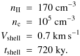
The parameters of a compressed shell around the ionised bubble can be determined thanks to equations presented in Appendix B related to H ii region theories. The input parameters are the ionising flux of the cluster (6 × 1047 ph s-1), the thickness of the shell (0.1 pc), and the observed radius of the shell (0.9 pc). These values lead to an initial density of 1.7 × 104 cm-3 back to ionisation onset, and a present electron density of 170 cm-3 in good agreement with the value deduced from radio continuum flux. Furthermore, we derive an H2 shell density of 5 × 104 cm-3. For an average column density of 3 × 1022 cm-2 for fronts 1 and 2 (without the dense clumps), it implies a depth of 0.2 pc. We conclude that front 1 and front 2 are parts of a ring around the ionised bubble, with a radius ~1 pc and a toroidal section of radius ~0.1–0.2 pc.
What could the original cloud geometry leading to a ring-confined bipolar H ii region be? The mass of ionised gas is of the order of 20 M⊙, taking a density of 200 cm-3 within a sphere of 0.9 pc in radius. Originally, this gas was in a neutral phase and progressively ionised by the massive stars at the centre of the cluster. If this mass was contained in a sphere with an initial density of 1.7 × 104 cm-3 (hence 3.4 × 104 cm-3 in H i), its diameter would have been 0.34 pc. Vela C presenting an elongated morphology, we propose that the massive stars in RCW 36 were born in a sheet confined by the hot low-dense neutral phase of the ISM and having a thickness of 0.34 pc at ionisation onset. An ionised bubble could expand into it, reaching a final density around 200 cm-3, while a ring of dense material will form only in the plane of the sheet. The extent in the horizontal direction of the sheet has to be ~2 pc to get the final ring. This means that we can estimate the initial dense ridge to have an H2 column density of ~1023 cm-2, a depth of ~2 pc and a thickness of ~0.3 pc. This result is in good agreement with observations of dense ridge in high-mass star-forming regions (e.g. Hennemann et al. 2012). Note that the pressure of the ionised gas is much bigger than the pressure in the hot ISM. Therefore, it is likely that the region will evolve into a bipolar H ii region with a morphology that strongly deviate from the spherical shape.
3.3. H ii region expansion in a molecular gas sheet
Using the electron density derived above, the pressure in the H ii region is estimated to be Pi/kB = 3 × 10⁶ K cm-3, where kB is the Boltzmann’s constant. Using a mean column density of 3 × 1022 cm-2, a diameter of 0.15 pc and a temperature around 20 K, as estimated from the column density and temperature maps, the mean pressure in the ring is about Pr/kB = 2 × 10⁶ K cm-3. In the densest parts where the column density reaches ~1023 cm-2 within 0.1-pc clumps, the pressure might reach 6 × 10⁶ K cm-3. These similar values suggest that the H ii region and the surrounding dense, molecular material that defines the ring-like morphology, may reach a pressure equilibrium, although the ring is still in supersonic expansion (1 pc/1 Myr ~ 1 km s-1, compared to a sound velocity ~0.4 km s-1 at 20 K). Using Eq. (B.4), the velocity of the H ii region shell is estimated to be 0.7 km s-1.
In the less dense parts, in particular at both ends of the Hα shell, the column density decreases to 5−10 × 1021 cm-2. No evidence is seen for shocks, or the presence of a dense dust shell. A possible explanation for this absence is that the density is very low at both ends of the Hα shell and the measured column density is dominated by local and galactic foregrounds and backgrounds. This explanation would imply that the H ii region may be freely expanding into the diffuse interstellar medium although it is probably confined at very large scales by the HI gas pressure. Heating of the dust over a large area will then be favoured in the East-West direction rather than in the North-South direction that is shielded by denser dust within the Centre-Ridge. This anisotropy would also explain the bipolar shape of the nebula as seen in the temperature map (Fig. 1c). The H ii region may have expanded inside a pre-existing elongated structure, either a filament or a sheet of molecular gas, that has been impacted by the UV ionisation. Assuming that the density of this pre-existing filament was proportional to r-2 in the East-West direction as reported in Arzoumanian et al. (2011) for interstellar filaments in IC 5146, Polaris and Aquila, then the ionised gas pressure due to the O9.5 star radiation becomes much greater than (i.e. 10 times) the gas pressure at a distance >0.3 pc from the star cluster in the E-W direction.
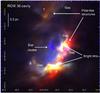 |
Fig. 3 Three-colour image of the RCW 36 sub-area focusing on the inner cavity of the ring-like structure as defined in Fig. 1c. Red is PACS 160 μm emission. Green is PACS 70 μm emission. Blue is IRAC 4.5 μm emission that here shows the star cluster distribution. Bright rims, pillar-like structures and 7 clumps appear prominent as well as large gaps between these structures. |
3.4. Structures in the ring
The Herschel and Spitzer IRAC observations allow the examination of the various structures of interstellar matter that comprise the environment of the RCW 36 at smaller scales (~0.1–0.2 pc). We focus in this paper on objects that are associated with pillar-like structures and bright rims. Seven areas with enhanced emission clearly stand out at the outer border of the cavity formed around the star cluster in Fig. 3. These clumps are identified in those figures by their number. Clumps 1, 2, 4, 5, 6 and 7 are associated in position with the observed bright-rims. Clump 3 coincides with a dark area on the Spitzer image and Hα map, which could be the backside of a pillar, seen in extinction in the NIR and Hα due to absorption by dust and in emission at 70 and 250 μm. This behaviour tells us that the observed emission features probably arise from areas at different distances and that pillar-like structures associated with the clumps have various orientations with respect to the star cluster. For instance, the bright-rimmed surfaces associated with clumps 1 and 2 would be behind the star cluster along the line-of-sight, while the dark areas associated with clumps 3, 6 and 7 would be in the foreground.
Interestingly, the bright-rims are found at the ends of pillar-like structures that are well separated by large gaps (see Fig. 3). The 70 μm emission traces the sides of the pillars closer to the star cluster. Peak emission seen at 70 and 250 μm (or 350, 450, 500 μm) is in general not coincident, while the optically thin emission at 250, 350 and 500 μm coincides more closely. This behaviour is clearly observed in clumps 1, 3, 4 and 5 (Figs. 4c, d). Given the various directional offsets, pointing errors cannot be the only explanation. In particular around clumps 4 and 5, 70-μm emission nicely traces three bright-rimmed structures also observed in the NIR, one corresponding to clump 4, another to clump 5 and the third in-between them in Fig. 4d. The 250-μm emission traces more deeply embedded structures, with distinct morphologies and positions clearly offset relative to the 70 μm and NIR emission peaks.
The source position offsets at various wavelengths suggest that emission at 4.5, 70, 160 and 250 μm (as well as 350 and 500 μm) trace distinct zones in the pillar-like structures, from bright-rimmed surfaces to internal regions. A possible reason for these differences is that these emission offsets reveal a temperature gradient from the photodissociation region (PDR) traced by the Hα emission to colder dust areas as detected at 250, 350 and 500 μm. We also note that the Hα emission encompasses the bright-rims around the star cluster and also arise in each lobe of the nebula (Fig. 1c). Another possible interpretation is that the 70-μm emission traces shocked, denser substructures ahead of the ionisation front and photodissociation region. The curved and bright-rimmed shape of the 70-μm emission corresponds to the inner border of a ring that is progressively photoionised by UV radiation from the star cluster. The bright-rimmed surfaces would then be the results of density enhancements in thin shells due to gas compression around the pillar-like structures (e.g. Tremblin et al. 2011). The sharp emission cut-off at the level of 40% of the peak flux seen in Fig. 4c suggests that 70-μm emission mainly arises from the surface of pillar heads rather than from inside. The clean western border also indicates that morphology and density could explain the 70-μm emission brightness in addition to the usual temperature gradient effects on dust emission.
3.5. Summary
In summary, the gas shell that surrounds the H ii region consists of an inhomogeneous medium, with a prominent ring-like structure of dense gas nearly perpendicular to the plane of the sky (see Fig. 5). The ring consists of many interstellar structures (bright rims, pillars, clumps) that have formed in between the shock and ionisation fronts, i.e. within the compressed gas ring that surrounds the star cluster and H ii region cavity. We now discuss what physical mechanism is the cause of their formation and how it is related to an initial filamentary cloud.
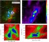 |
Fig. 4 a) Three-colour image of the RCW 36 cavity (see Fig. 1) corresponding to the field mapped by P-ArTéMiS. Red is the column density that is shown for values between 3 × 10²¹ and 5 × 1022 cm-2 to limit the dynamics and emphasize low density features. The peak column density is 1.7 × 1023 cm-2. Green is the IRAC 4.5 μm image that shows structures due to extinction or emission near the star cluster. Blue is the 2MASS K-band image that shows the young stars. The 7 clumps as described in the text are numbered from 1 to 7 on this image. The two rectangular areas in dashed white lines represent the regions mapped in c) and d). b) Column density map combining Herschel and p-ArTéMiS observations. c) PACS 70-μm emission (colour image and blue contours) with SPIRE 250-μm emission overlaid (in yellow) contours (levels: 10, 20, 30, 40, 50, 60, 70, 80, and 90% of 250 Jy beam-1 peak emission) for clumps 1 and 2. d) Same as b) but for clumps 3, 4 and 5. Position offsets between 70 and 250 μm emission are clearly observed. |
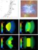 |
Fig. 5 Illustration of the proposed scenario. Observations: a) Schematic view of the initial ridge as derived in Sect. 3.2. b) Modelled ring superimposed on the Herschel 3-colour image. Numerical simulations: c) Cut through the plane of the initial ridge. The radius of the yellow circular section is 1 pc. The density is given in H i cm-3. d) Cut through the plane of the ridge after ionisation reshaped it and formed a ring. e) Cut of d) from above. The bipolar shape clearly appears. f) Cut of d) from the backside. The ridge/filament projected shape clearly appears. The orientation of each cut is given by x, y, z axes on each image. |
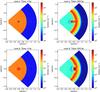 |
Fig. 6 Numerical simulations. Each box shows a cut of the density map (φ = 0) before or after the ionisation of a slab of interstellar gas. a) A clump with a density of 3 × 105 cm-3 is embedded in the slab of interstellar gas. Radiation from the O9.5 star comes from the position (0, 0). b) After 0.6 Myr, the ionisation has led to the formation of a pillar. The base of the pillar is located within the compressed shell, in between the ionisation and shock fronts. The head of the pillar remains nearly at the position of the initial clump. c) A larger clump with a lower density is ionised by the O9.5 photon flux. d) A clump is formed within the compressed shell with a hole around it. |
4. Modelling the RCW 36 nebula and its structures
4.1. Global scale modelling
In Sect. 3, we proposed a geometry of RCW 36 consisting of a ring centred around the star cluster and perpendicular to the bipolar lobes. Using an analytical 1D-model for H ii region evolution (Appendix B), we deduce the physical characteristics of the initial ridge that was reshaped by ionisation (see Fig. 5a,b). In this section, dedicated 3D numerical simulations are employed to model the process turning a dense ridge into a bipolar nebula.
We have employed the HERACLES2 code (Gonzalez et al. 2007), a three-dimensional (3D) numerical code solving the equations of hydrodynamics that has been coupled to the ionisation as described in Tremblin et al. (2012a). We take for initial conditions the parameters deduced from Sect. 3.2 i.e., a cluster emitting 6 × 1047 s-1 inside a ridge (or a sheet) that is 0.34 pc large and extents up to 1 pc on each side of the cluster. The H2 density of the ridge is 1.7 × 104 cm-3 (3.4 × 104 cm-3 in H i for the simulation). The geometry of the mesh is spherical. The radius extents from 0.1 pc to 1.5 pc, the polar angle θ from 45° to 135°, and the azimuth angle φ between –45° and +45°. The number of cells is 1003. The boundary conditions are reflexive at the inner radius, free flow at the outer radius, and periodic in the other directions. The adiabatic index γ is set to 1.01 allowing us to treat both the hot ionized gas and the cold unionized one as two different isothermal phases. The simulation is ran until the shocked layer reached a radius of 1 pc. A 3D view of the output of the simulation is shown in Fig. 5c, d with an orientation comparable to the observed ring in Fig. 5b. The density and the width of the ring as well as the density in the ionised region are in good agreement with the parameters that was deduced from the 1D analytical formulae in Sect. 3.2. Another view (Fig. 5e) illustrates the bipolar morphology of the H ii region formed in the simulation, with the two lobes on each side of the dense ring. Interestingly, such a morphology would appear as a ridge or a filament on the sky if observed edge-on (Fig. 5f).
The only difference with the 1D model in an homogeneous medium is the velocity of the shell and the time at which the radius of 1 pc is reached. In the 3D case, the velocity of the shell is around 1.4 km s-1 (1-pc radius reached in 600 ky) while it was only 0.7 km s-1 in the 1D case (1-pc radius reached in 750 ky). This difference can be easily understood in terms of rocket motion. The analytic formula in Appendix B gives a shell velocity that always decreases with time for the collect process in an homogeneous medium. In our 3D simulation, the ridge has a thickness that gives enough material to the ionised bubble to reach an electron density around 200 cm-3. Nevertheless some ionised gas is evacuated from the 1-pc radius bubble through the extended lobes (see Fig. 5). Therefore the ionisation at the front will increase and will accelerate the shell so that the velocity remains almost constant around 1.4 km s-1.
Gravity was not included in the numerical simulations. The kinetic energy of the expanding shell dominates its gravitational energy by a large factor at early ionisation phases and still in the present observed situation. Nonetheless star cluster gravity may affect the H ii region expansion in the future.
4.2. Triggered formation of pillars and clumps
In Sect. 3.4, we surmised that the various morphological features in the RCW 36 area could result from the ionisation of a section of a pre-existing ridge. Nonetheless, it was not clear whether the clumps were already inside the filament or whether they formed in the ionisation/shock shell with their bright rim counterparts. We have employed the simulations to test the two possibilities.
Figure 6a presents the initial conditions of clump existing before the impact of ionisation on the filament. A dense and small spherical clump (0.1 pc in diameter, 3 × 105 cm-3, 20 times the density in the initial filament) was embedded in the slab of interstellar gas. Such physical conditions corresponded to those observed in the Herschel map where the clump column density reached 1023 cm-2 within 0.1 pc. Figure 6b shows the result after 0.6 Myr, the ionising front pushed away the gas by 1 pc and an elongated pillar formed due to the dense clump resistance inducing a curvature in the shock front. Tremblin et al. (2012a) discussed the role of shock curvature in forming pillars. The pillar head was nearly at the location of the clump in this model.
Figure 6c illustrates the second situation, where the spherical clump was wider (0.1 pc in diameter) and less dense (5 × 104 cm-3), i.e. 3 times the density in the initial filament. Instead of forming an elongated pillar, the ionisation front produced a more compact structure than in the first situation. Large gaps on each side of the compact clump were also formed (Fig. 6d), which are consistent with the large gaps observed in Fig. 3.
The perturbation, caused by ionisation, triggered local curvature of the ionisation and shock fronts. This process was already identified in Tremblin et al. (2012) as the key process to form pillars, i.e., when the induced curvature is sufficient to make the shell collapse on itself. When the clumpy inhomogeneity is large in size and at a lower density, however, the curvature is not sufficient to trigger a collapse, but rather leads to gas flows in the shell perpendicular to the propagation of the ionising flux. These flows are accelerated with the shell and will form dense clumps and gaps that will remain in the shell during the 0.6 Myr of expansion.
In summary, ionisation of very dense inhomogeneities can lead to long pillar morphology. Ionisation of inhomogeneities only slightly denser than the ambient molecular gas lead to very compact clumps with a large gaps around them. Clumps 4, 5, 6, and 7, given the orientation of the associated pillar-like structures (Fig. 3), correspond to the second case. The orientations of clumps 1, 2, and 3 do not exclude the possibility that they are much larger than observed in projection, and are in fact large pillars seen head-on. However, the large gaps around these objects suggest that their formation is better explained by the second case scenario in Figs. 6c, d. Therefore, the observed pillar-like structures must result from the compression of only slightly denser inhomogeneities in a pre-existing filament due to the ionisation/shock front.
5. Second generation of star formation
The seven clumps (as seen in Fig. 3) are areas with enhanced emission that could result from density enhancements due to compression induced by the ionisation (see Sects. 3.4 and 4.2). They may be potential sites of star formation. Thanks to our Herschel data in five bands, it is possible to characterise the temperature and mass of these clumps, and hence test whether they could be the progenitors of new stars. Nonetheless, the various positional source offsets from 70 to 250 μm make difficult the clear identification of any single sources in RCW 36 at the given wavelengths, as also noticed by Giannini et al. (2012) in their star formation census towards Vela C. This behaviour precludes the use of a spectral energy distribution fit as an accurate identification tool of the protostellar nature of the sources without extrapolating the measured flux at a given wavelength for a predefined area. With the ambiguities between the contribution of each substructures (bright rims, clumps), extrapolating flux values is not easy, especially at 70 μm. Focusing on the optically thin dust emission observed with sufficient angular resolution is a better option.
Derived and observed physical parameters of the Vela C region, initial ridge, H ii region and ring.
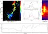 |
Fig. 7 a) CS (1–0) velocity map around RCW 36 in Vela C with column density contours overlaid (levels: 5, 15, 25, 35, and 45% of the 1.8 × 1023 cm-2 column density). b) CS(1−0) integrated spectra around RCW 36. The spectra are spatially integrated in the coloured circles showed in Fig. 2a. CS (blue) and C34S (red) lines towards pillar 1 are presented in the bottom panel. c) Position−velocity diagram for a shell, which is expanding radially beyond the clumps. The diagram is built by taking the mean velocity around a circle for a given radius (the angular offset). Each circle is centred on the star cluster. The colour indicates the line intensity. d) Velocity−position diagramme for the area in Fig. 7a based on the vertical profile of the CS velocity, which is averaged horizontally. 0 offset corresponds to RCW 36. |
The gas and dust mass of the clumps embedded in the pillar-like structures described in Sect. 3 can, however, be estimated by considering the integrated flux at 350 μm. We modelled the dust emission flux with a Planck function and a dust opacity per unit (gas + dust) mass column density of 0.07 cm2 g-1, which allows deduction of the dust mass (see Minier et al. 2009, for details). The dust temperature range is first estimated with the temperature map in Hill et al. (2011). Given the uncertainties on the temperature values around RCW 36, the mass values are derived for a temperature range of 17–25 K. M25′′ is the total mass estimated over an area of ~25″ in diameter, i.e. 0.09 pc at 700 pc, which corresponds to the Herschel beam at 350 μm. M25′′ vary from ~4 to 72 M⊙ across the seven clumps, which is in relative agreement with results by Giannini et al. (2012) and Hill et al. (2011). Clump 1 is the most massive. A Gaussian fit was applied to the 350 μm emission image at the position of each dust clump embedded in the pillar-like structures. Clumps 1, 2, 3 and 7 are well fitted while the fitting procedure does not converge for clumps 4, 5 and 6. From the Gaussian fits, the level of a diffuse emission component was estimated and substracted from the measured fluxes. The derived masses (M) using these corrected fluxes are also given in Table 2. M6000 AU are masses estimated inside an area of 6000 AU or 0.03 pc in diameter, i.e. the typical fragmentation length-scale observed in nearby cluster-forming regions (Peretto et al. 2007; Longmore et al. 2006), using the corrected peak flux and a density profile in r-2 (as in Minier et al. 2009). Another way of deriving the clump masses was based on the use of the combined Herschel 160 μm and p-ArTéMiS 450 μm data (Fig. 4b). This method can produce a column density map with better angular resolution (12″) than the Herschel single one (36″). It is possible to fit the column density over each clump area with a 2-dimensional Gaussian curve and obtain a second estimate of the clump masses (MNH2 listed as in Table 2). However, as noted in Sect. 2, the method remains approximate.
Comparing MNH2 and M values, estimates made with either method are consistent within a factor of 2. Differences can be explained by different dust temperatures and higher angular resolution in the combined Herschel and p-ArTéMiS map, which results in a better Gaussian fit of the column density area associated with each clump. If the emission arises from dusty envelopes around protostar candidates, the derived masses indicate that clumps 1, 2, 3 and 7 could form low-mass to intermediate-mass stars, possibly high-mass stars in the case of clump 1. It is, however, difficult to exhibit evidence for on-going star formation. Recent SINFONI/VLT observations of RCW 36 (Ellerbroek et al. 2011) have revealed two young stellar objects (YSOs) coincident in position with clump 1. These YSOs are also seen in the Spitzer/IRAC images. One of the YSOs is identified as a K5 star in preliminary work using the SINFONI data by Paalvast (2011). Given the high density of the clump, the visual extinction Av is ~100, leading to high extinction in the near infrared. The two YSOs, as observed in the near infrared, are probably located in front of clump 1 rather than inside it. Their colours suggest that they were formed with the star cluster and therefore belong to the first generation of stars (see the star cluster distribution, Fig. 7 in Baba et al. 2004). This placement also confirms that clump 1 is located behind the star cluster along the line-of-sight.
A second generation of star formation in the RCW 36 area is possibly preparing to emerge from the dense clumps 1, 2, 3 and 7. Uncertainties remain on the mass of the future stars to be formed, if any.
Masses of the seven clumps.
6. Discussion
6.1. Kinematics and the 3-dimensional model of RCW 36
We have modelled RCW 36 as a ring of molecular gas expanding with the H ii region. As noted in Sects. 3 and 4, the emission of pillar-like structures, clumps and bright rims tells us about their orientation, and their various distances relative to the star cluster. Figure 5 presents the orientation of the ring. Clumps 1 and 2 are for instance located behind the star cluster, nearly head-on. Pillar-like structure 7 is located on the outer layer of the ring.
The velocity field can put further constraints on the expanding motion in RCW 36. This area has recently been mapped in CS(1−0) with the Mopra telescope. The corresponding velocity map is presented in Fig. 7a. When comparing the velocity map with the column density map (Fig. 1a), the Northern region is mainly redshifted and Southern one is mainly blueshifted, both with respect to an average velocity around 7 km s-1. The velocity spans a range of 4–9 km s-1. This gradient might suggest some North-South global motion in the direction of RCW 36. Nonetheless, small velocity gradients also appear locally on the CS velocity map in the environment of RCW 36, suggesting that small-scale motions are also at play. Similar lateral gradients are observed in the DR21 filament dynamics (Schneider et al. 2010; White et al. 2010).
In the case of RCW 36, lateral gradients are observationally explained by multiple line profiles in CS(1−0) spectra. Clump 1 for instance presents clear double line profiles with a peak at 6.5 and the other at 8 km s-1. Very weak emission is detected in the optically thin C34S(1−0) line with double peaks, as well, which correspond in velocity with the CS line maxima (Fig. 7b). These two components would indicate that the CS line is partly optically thin and that the double line profile signposts two distinct geographical areas within the telescope beam, one approaching us, the other receding. Similar profiles in CS are seen towards clumps 2 and 7 while CS is single-peaked in clumps 3, 4, 5 and 6.
CS spectra have been integrated in four different locations in the ring-like structure around RCW 36 (see Fig. 2a). The corresponding spectra are shown in Fig. 7b. The yellow and green spectra are integrated on the front 2, and the blue and black spectra on the front 1. The four zones present a component at 7 km s-1 corresponding to the systemic velocity of the ridge area. In addition to that component, the yellow spectrum on the front 2 has a blue-shifted component at 5 km s-1 and the blue spectrum on the front 1, a red-shifted component at 8 km s-1. Recall that from the Hα emission (see Fig. 2a), it is possible to infer that the front 1 is behind the star cluster and the front 2 in front of it. Therefore the velocity shifts are not the signature of infall and can be interpreted as the outward expansion of the ring at a velocity between 1 and 2 km s-1. The green and black areas expand on the north-south axis that is perpendicular to the line of sight. Therefore their velocity spectra are coherent with an expansion. The velocity of the shell as derived from the 3D numerical simulations is ~1.4 km s-1 and is in relatively good agreement with the velocity inferred from the CS data. Finally, when measuring the CS gas velocity inside a circular area centred on the star cluster and encompassing the clumps, a profile is seen that suggests the clumps are located on an expanding front (Fig. 7c). Their radial velocities fall within a rough C-shape in the velocity versus radius diagram that is typical of radially-measured spherical expansion (e.g. Purcell et al. 2009).
In conclusion, the kinematic analysis of RCW 36 leads to an interpretation of the velocity field consistent with an expanding ring of molecular gas under ionising pressure.
6.2. Ionisation impact and feedback
We have shown in Sect. 4 that gas structures observed in the compressed shell around the H ii region, such as pillar-like structures, bright rims and clumps, teach us what occurred in the parent molecular cloud. The shape of the bright-rimmed clouds as observed in Fig. 3, with a base corresponding in position with the H ii region shell and a head pointing towards the star cluster, can be compared to the results in Tremblin et al. (2012a,b): these can explain the formation of pillar-like structures, including clumps around the H ii region shell, by ionisation, turbulence and lateral shocks on a curved molecular border that is not homogeneous in density (e.g. Deharveng et al. 2010; Thompson et al. 2004; Hester et al. 1996, for observational examples). Numerical simulations including turbulence (Tremblin et al. 2012b) suggest that ionisation-triggered structures include globules and pillars for high Mach number (>2) (e.g. Schneider et al. 2012b) and very compact, pillar-like clumps for low Mach number. RCW 36 in Vela C would then be a quiet region in terms of turbulence that is dominated by ionisation.
Dedicated simulations for RCW 36 in Sect. 4.2, including ionisation only, provide explanation of the processes that led to the observed clumps and pillar-like structures. Our simulations suggest that very dense clumps such as clump 1 could not have pre-existed because they would have formed long pillars otherwise. Since the clumps are located in the H ii region shell, their formation was triggered by instabilities in the ionisation/shock front. They are then accelerated with the shell and stay at the edge of the H ii region. This interpretation is consistent with recent statistics on the location of the dense clumps around star cluster including young massive stars that show that they tend to be around the H ii region (Thompson et al. 2011; Deharveng et al. 2010).
Based on this study, we propose that the impact of radiative feedback on the star-formation rate could be “positive”. Such a result was also pointed out in other numerical simulations of implosion of isothermal spherical clouds using smoothed particle hydrodynamics (SPH) codes (e.g. Miao et al. 2006; Gritschneder et al. 2009). However, our scenario differs from the radiative-driven implosion of a spherical clump as we argue that bright-rims and pillars do not form from an isolated, pre-existing dense clumps, but from only slightly denser inhomogeneities in an interstellar filament. Indeed, ionisation does not disperse cores that have already formed, pillars will form around them, and density perturbations in the cloud lead to the formation of new clumps inside the dense shell. In the case of RCW 36, the ionisation-triggered clumps are sufficiently dense to lead to star formation. Ionisation feedback induces the formation of clumps, and possibly stars inside them.
7. Conclusions and summary
In this paper, we have investigated the role of ionising stars in reshaping the RCW 36 area through morphological and kinematical signatures. In particular, we have showed that, locally, a filament in a column density map near an ionising star cluster could be described as a more complex structure of interstellar matter than a linear one. Indeed, projection effects along the line-of-sight, which could lead to apparent alignments of interstellar gas structures from distinct distances, are known to cause major issues in deriving a mass-size relationship based on a line velocity analysis (Shetty et al. 2010). We may face similar issues when interpreting local morphologies at (sub)parsec scales in a column density map.
Starting from the Herschel observations of interstellar filaments in Vela C that were statistically analysed by Hill et al., our dedicated study of the RCW 36 area offers a way of understanding a complex interstellar morphology as the natural evolution of a filamentary one. Thanks to the relatively close location of the Vela C molecular cloud and in light of dedicated numerical simulations, we are able to propose a clear view of the radiative feedback impact on an interstellar filament, including the physical mechanisms that lead to the formation of bright rims and pillars-like structures as well as the triggered formation of dense star-forming clumps at the borders of the H ii region.
In summary, the overall morphology of RCW 36 results from the ionisation of a filamentary structure, that was oriented North-South similarly to Centre-Ridge in Vela C. Our results demonstrate that the RCW 36 environment is the scene of (1) the ionisation of an initial molecular ridge or sheet by a star cluster; (2) the expansion of an associated H ii region; followed by (3) the formation of a ring in the sheet plane and bipolar lobes in the perpendicular plane; (4) the emergence of bright-rims and pillar-like structures; and (5) the triggered formation of star-forming clumps. Such results demonstrate that, locally, filamentary structures mark the location of very dynamical phenomena.
We conclude that the detailed analysis of the pillar-like structures leads to a better knowledge of the initial conditions that dominated in the parent molecular cloud. We propose that a morphological diagnostic of ionisation-triggered structures near the compressed gas shells associated with H ii regions could lead to better understanding of the physical process in action, including the turbulence role and the trigger of a new generation of stars.
Beyond the study of Vela C, these results could apply to understanding better bipolar nebulae as the results of H ii region expansion within a molecular ridge or an interstellar filament. Ionisation-triggered structures could be used generally as tools to disentangle physical phenomena at play in a molecular cloud under the influence of high-mass star radiative feedback.
Online material
Appendix A: DisPerSe and filament fitting
The DisPerSe algorithm (Sousbie 2011) was used with an intensity contrast level of 1021 cm-2 and a low-density threshold of 2 × 1022 cm-2. These parameters are taken to trace the crests of the main parts of the dense fronts that can be identified by eye on the column density map. Then we performed transverse column density profiles along a piecewise linear segmentation of the DisPerSe skeleton. We also fitted the inner part of the profiles with Gaussian functions (similarly to Arzoumanian et al. 2011) after subtracting a background set at the minimum of the fitted profile. The level of the background does impact the width of the Gaussian profile. However, other choices of the background level only induce small variations of the width (Peretto et al. 2012). There are two possibilities to determine the full width at half maximum (FWHM), fitting Gaussian profiles at each position along the front and take the mean value or fitting a Gaussian profile on the averaged profiles. We used both strategies and the corresponding deconvolved FWHM values are in good agreement (0.10 ± 0.02 pc for the front 1 at a resolution 12″ and 0.20 ± 0.02 pc for the front 2 at a resolution of 36″ to compare with the values indicated in Fig. 2).
Appendix B: Collect theory in a homogeneous medium
Based on the works of Elmegreen et al. (1977) and Spitzer (1978), we derive an analytical expression for the different parameters of an H ii region shell: its velocity Vshell, its density nc, its thickness Lshell and its radius rshell.
For simplicity we suppose that the velocity of the ionisation front (I-front) and shock
front (S-front) are the same and are equal to Vshell. The
cold medium (n0, v0 = 0) is
separated from the compressed shell (nc,
vc) by the S-front. The compressed shell is separated from
the ionised gas (nII, vII) by
the I-front. All the parameters are resumed in the schematic view in Fig. B.1. The isothermal Rankine-Hugoniot conditions in the
referential of the cold gas gives 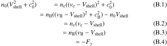 with
Fγ the ionisation flux at the I-front
(taking in account the recombination in the ionised gas). These relations are local and
we neglect the curvature of the fronts, besides the shell is assumed stationary in the
referential of the cold gas. Since the shock is strongly supersonic, the second equation
can be approximated by
with
Fγ the ionisation flux at the I-front
(taking in account the recombination in the ionised gas). These relations are local and
we neglect the curvature of the fronts, besides the shell is assumed stationary in the
referential of the cold gas. Since the shock is strongly supersonic, the second equation
can be approximated by  (B.5)with
ζ = 2 for a D-critical I-front
(Vshell − vII =
cII) and ζ varies from 2 to 1 in the weak
D phase. The time-scale of the expansion of the shell is much longer than the ionisation
time-scale, therefore the equilibrium between ionisation and recombination holds during
the expansion
(B.5)with
ζ = 2 for a D-critical I-front
(Vshell − vII =
cII) and ζ varies from 2 to 1 in the weak
D phase. The time-scale of the expansion of the shell is much longer than the ionisation
time-scale, therefore the equilibrium between ionisation and recombination holds during
the expansion
 |
Fig. B.1 Outline of the collect and collapse scenario with the different variables used in the analytical model. |
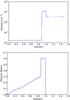 |
Fig. B.2 Density and velocity profile of a 1D spherical simulation of the ionization of a homogeneous medium in the conditions of RCW 36. The radius is between 0 and 1.5 pc with 2000 cells. The initial density is 3.4 × 104 cm-3, the ionizing flux 6 × 1047 ph s-1 and the simulation is run during 720 ky. |
 (B.6)with
Rs the Strömgren radius at the end of the R-type phase and
rshell the position of the shell at a
time t in the D-type phase. Therefore from Eqs. (B.5) and (B.6), we get
(B.6)with
Rs the Strömgren radius at the end of the R-type phase and
rshell the position of the shell at a
time t in the D-type phase. Therefore from Eqs. (B.5) and (B.6), we get 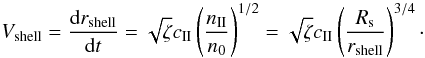 (B.7)By integration we
get the position of the shell and we set ζ to 1 (weak D-type I-front)
to get back the result from Spitzer (1978)
(B.7)By integration we
get the position of the shell and we set ζ to 1 (weak D-type I-front)
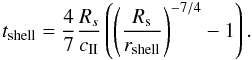
to get back the result from Spitzer (1978) 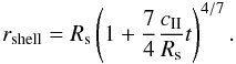 (B.8)This is the quickest
way to obtain the position of the shell that was obtained by Spitzer
(1978). The age of the H ii region can be deduced from
(B.8)This is the quickest
way to obtain the position of the shell that was obtained by Spitzer
(1978). The age of the H ii region can be deduced from
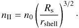
 (B.9)The density in
the shell nc can be obtained with Eq. (B.5)
(B.9)The density in
the shell nc can be obtained with Eq. (B.5)
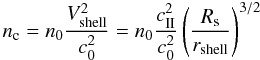 (B.10)and
the density in the H ii region
(B.10)and
the density in the H ii region
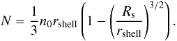
 (B.11)It is interesting
to note that the compression decreases with time. The column density N
in the shell is equal to what has been accumulated during the collect phase:
n0rshell/3 minus what remains
in the H ii region:
nIIrshell/3
(B.11)It is interesting
to note that the compression decreases with time. The column density N
in the shell is equal to what has been accumulated during the collect phase:
n0rshell/3 minus what remains
in the H ii region:
nIIrshell/3
 (B.12)The thickness of the
shell Lshell is then given by
N/nc
(B.12)The thickness of the
shell Lshell is then given by
N/nc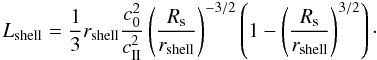 (B.13)\newpage\noindentThis
expression only depends on the shell radius and the Strömgren radius. Thus the shell
thickness and radius can be used to infer the initial Strömgren radius and the initial
density in the medium. For a shell thickness of 0.1 pc and a shell radius of 0.9 pc, the
initial H i density of the medium is 3.4 × 104 cm-3.
All the other parameters can be deduced from this density
(B.13)\newpage\noindentThis
expression only depends on the shell radius and the Strömgren radius. Thus the shell
thickness and radius can be used to infer the initial Strömgren radius and the initial
density in the medium. For a shell thickness of 0.1 pc and a shell radius of 0.9 pc, the
initial H i density of the medium is 3.4 × 104 cm-3.
All the other parameters can be deduced from this density
 (B.14)We
compared these results with a one-dimensional spherical simulation performed with the
Heracles code (radius between 0 and 1.5 pc with 2000 cells). We took an initial density
at 3.4 × 104 cm-3, a flux of
6 × 1047 ph s-1 and run the simulation during 720 ky to reach
the observed shell radius of 0.9 pc. The density and velocity profiles are given in Fig.
B.2. In the simulation, the averaged ionised-gas
density is 170 cm-3, the compressed gas density
1.1 × 105 cm-3, the shell velocity 0.61 km s-1, and
the shell thickness 0.11 pc. The results from our simple analytical approach and the
simulation are in a good agreement (no more than 10% difference).
(B.14)We
compared these results with a one-dimensional spherical simulation performed with the
Heracles code (radius between 0 and 1.5 pc with 2000 cells). We took an initial density
at 3.4 × 104 cm-3, a flux of
6 × 1047 ph s-1 and run the simulation during 720 ky to reach
the observed shell radius of 0.9 pc. The density and velocity profiles are given in Fig.
B.2. In the simulation, the averaged ionised-gas
density is 170 cm-3, the compressed gas density
1.1 × 105 cm-3, the shell velocity 0.61 km s-1, and
the shell thickness 0.11 pc. The results from our simple analytical approach and the
simulation are in a good agreement (no more than 10% difference).
We define a “pillar-like structure” as a dust emission morphology that consists of a roughly elongated body of ~0.1 to 1 pc in extent with a convex head and large gaps around it. See Tremblin et al. (2012a) for a complete morphology overview.
Acknowledgments
The Herschel spacecraft was designed, built, tested, and launched under a contract to ESA managed by the Herschel/Planck Project team by an industrial consortium under the overall responsibility of the prime contractor Thales Alenia Space (Cannes), and including Astrium (Friedrichshafen) responsible for the payload module and for system testing at spacecraft level, Thales Alenia Space (Turin) responsible for the service module, and Astrium (Toulouse) responsible for the telescope, with in excess of a hundred subcontractors. SPIRE has been developed by a consortium of institutes led by Cardiff Univ. (UK) and including Univ. Lethbridge (Canada); NAOC (China); CEA, LAM (France); IFSI, Univ. Padua (Italy); IAC (Spain); Stockholm Observatory (Sweden); Imperial College London, RAL, UCL-MSSL, UKATC, Univ. Sussex (UK); Caltech, JPL, NHSC, Univ. Colorado (USA). This development has been supported by national funding agencies: CSA (Canada); NAOC (China); CEA, CNES, CNRS (France); ASI (Italy); MCINN (Spain); SNSB (Sweden); STFC and UKSA (UK); and NASA (USA). PACS has been developed by a consortium of institutes led by MPE (Germany) and including UVIE (Austria); KU Leuven, CSL, IMEC (Belgium); CEA, LAM (France); MPIA (Germany); INAF-IFSI/OAA/OAP/OAT, LENS, SISSA (Italy); IAC (Spain). This development has been supported by the funding agencies BMVIT (Austria), ESA-PRODEX (Belgium), CEA/CNES (France), DLR (Germany), ASI/INAF (Italy), and CICYT/MCYT (Spain). The Mopra radio telescope is part of the Australia Telescope National Facility which is funded by the Commonwealth of Australia for operation as a National Facility managed by CSIRO. The UNSW-MOPS Digital Filter Bank used for the observations with the Mopra Telescope was provided with support from the University of New South Wales, Monash University, University of Sydney and Australian Research Council. This work is based in part on observations made with the Spitzer Space Telescope, which is operated by the Jet Propulsion Laboratory, California Institute of Technology under a contract with NASA. N.L. acknowledges support from Région Ile de France and partial support from Center of Excellence in Astrophysics and Associated Technologies (PFB 06) and Centro de Astrofísica FONDAP 15010003. D.E. and K.L.J.R. are funded by an ASI fellowship under contract number I/005/11/0. This work was granted access to the HPC resources of [CCRT/CINES/IDRIS] under the allocations c2011042204 and c2012042204 made by GENCI (Grand Équipement National de Calcul Intensif). We acknowledge Christophe Carreau’s (ESTEC/ESA) help in producing Fig. 1b.
References
- André, P., Minier, V., Gallais, P., et al. 2008, A&A, 490, L27 [NASA ADS] [CrossRef] [EDP Sciences] [Google Scholar]
- André, P., Men’shchikov, A.,Bontemps, S., et al. 2010, A&A, 518, L102 [NASA ADS] [CrossRef] [EDP Sciences] [Google Scholar]
- Arzoumanian, D., André, P., Didelon, P., et al. 2011, A&A, 529, L6 [Google Scholar]
- Baba, D., Nagata, T., Nagayama, T., et al. 2004, ApJ, 614, 818 [NASA ADS] [CrossRef] [EDP Sciences] [Google Scholar]
- Bally, J., Chun Yu, K., & Zinnecker, H. 1998, AJ, 116, 1868 [NASA ADS] [CrossRef] [Google Scholar]
- Caswell, J., & Haynes, R. F. 1987, A&A, 171, 261 [NASA ADS] [Google Scholar]
- Condon, J. J., Griffith, M. R., & Wright, A. E. 1993, AJ, 106, 1095 [NASA ADS] [CrossRef] [Google Scholar]
- Deharveng, L., Schuller, F., Anderson, L. D., et al. 2010, A&A, 523, A6 [NASA ADS] [CrossRef] [EDP Sciences] [Google Scholar]
- Dale, J. E., & Bonnell, I. 2012, MNRAS, 422, 1352 [NASA ADS] [CrossRef] [Google Scholar]
- Ellerbroek, L. E., Kaper, L., Bik, A., et al. 2011, ApJ, 732, 9 [Google Scholar]
- Elmegreen, B. G., & Lada, C. J. 1977, ApJ, 214, 725 [NASA ADS] [CrossRef] [Google Scholar]
- Flagey, N., Boulanger, F., Noriega-Crespo, A., et al. 2011, A&A, 531, A51 [NASA ADS] [CrossRef] [EDP Sciences] [Google Scholar]
- Giannini, T., Elia, D., Lorenzetti, D., et al. 2012, A&A, 539, A156 [NASA ADS] [CrossRef] [EDP Sciences] [Google Scholar]
- Gonzalez, M., Audit, E., & Huynh, P. 2007, A&A, 464, 429 [NASA ADS] [CrossRef] [EDP Sciences] [Google Scholar]
- Griffin, M. J., Abergel, A., Abreu, A., et al. 2010, A&A, 518, L3 [Google Scholar]
- Gritschneder, M., Naab, T., Burkert, A., et al. 2009, MNRAS, 393, 21 [NASA ADS] [CrossRef] [Google Scholar]
- Hambly, N. C., MacGillivray, H. T., Read, M. A., et al. 2001, MNRAS, 326, 1279 [NASA ADS] [CrossRef] [Google Scholar]
- Hester, J. J., Scowen, P. A., Sankrit, R., et al. 1996, AJ, 111, 2349 [NASA ADS] [CrossRef] [Google Scholar]
- Hill, T., Motte, F., Didelon, P., et al. 2011, A&A, 533, A94 [NASA ADS] [CrossRef] [EDP Sciences] [Google Scholar]
- Hill, T., Motte, F., Didelon, P., et al. 2012, A&A, 542, A114 [NASA ADS] [CrossRef] [EDP Sciences] [Google Scholar]
- Longmore, S. N., Burton, M. G., Minier, V., & Walsh, A. J. 2006, MNRAS, 369, 1196 [NASA ADS] [CrossRef] [Google Scholar]
- Mampaso, A., Vilchez, J. M., Pismis, P., & Phillips, J. P. 1987, RMxAA, 14, 474 [NASA ADS] [Google Scholar]
- Martin-Hernandez, N. L., Vermeij, R., & van der Hulst, J .M. 2005, A&A, 433, 205 [NASA ADS] [CrossRef] [EDP Sciences] [Google Scholar]
- Massi, F., Lorenzetti, D., & Giannini, T. 2003, A&A, 399, 147 [NASA ADS] [CrossRef] [EDP Sciences] [Google Scholar]
- Mezger, P. G., Sievers, A. W., Haslam, C. G. T., et al. 1992, A&A, 256, 631 [NASA ADS] [Google Scholar]
- Miao, J., White, G. J., Nelson, R., Thompson, M., & Morgan, L., 2006, MNRAS, 369, 143 [NASA ADS] [CrossRef] [Google Scholar]
- Minier, V., André, P., Bergman, P., et al. 2009, A&A, 501, 1 [Google Scholar]
- Molinari, S., Swinyard, B., Bally, J., et al. 2010, A&A, 518, L100 [NASA ADS] [CrossRef] [EDP Sciences] [Google Scholar]
- Motte, F., Zavagno, A., Bontemps, S., et al. 2010, A&A, 518, L77 [NASA ADS] [CrossRef] [EDP Sciences] [Google Scholar]
- Murphy, D. C., & May, J. 1991, A&A, 247, 202 [NASA ADS] [Google Scholar]
- Panagia, N. 1973, AJ, 78, 929 [NASA ADS] [CrossRef] [Google Scholar]
- Paalvast, M. 2011, Bachelor Report, University of Amsterdam [Google Scholar]
- Peretto, N., Hennebelle, P., & André, P. 2007, A&A, 464, 983 [NASA ADS] [CrossRef] [EDP Sciences] [Google Scholar]
- Peretto, N., André, Ph., Könyves, V., et al. 2012, A&A, 541, A63 [NASA ADS] [CrossRef] [EDP Sciences] [Google Scholar]
- Pilbratt, G. L., Riedinger, J. R., Passvogel, T., et al. 2010, A&A, 518, L1 [CrossRef] [EDP Sciences] [Google Scholar]
- Poglitsch, A., Waelkens, C., Geis, N., et al. 2010, A&A, 518, L2 [NASA ADS] [CrossRef] [EDP Sciences] [Google Scholar]
- Purcell, C., Minier, V., Longmore, S., et al. 2009, A&A, 504, 139 [NASA ADS] [CrossRef] [EDP Sciences] [Google Scholar]
- Rodger, A. W., Campbell, C. T., & Whiteoak, J. B. 1960, MNRAS, 121, 103 [NASA ADS] [CrossRef] [Google Scholar]
- Schneider, N., Csengeri, T., Bontemps, S., et al. 2010, A&A, 520, A49 [NASA ADS] [CrossRef] [EDP Sciences] [Google Scholar]
- Schneider, N., Csengeri, T., Hennemann, M., et al. 2012a, A&A, 540, L11 [NASA ADS] [CrossRef] [EDP Sciences] [Google Scholar]
- Schneider, N., Güsten, R., Tremblin, P., et al. 2012b, A&A, 542, L18 [Google Scholar]
- Sousbie, T. 2011, MNRAS, 414, 350 [NASA ADS] [CrossRef] [Google Scholar]
- Shetty, R., Collins, D. C., Kauffmann, J., et al. 2010, ApJ, 712, 1049 [NASA ADS] [CrossRef] [Google Scholar]
- Spitzer, L. 1978, in Physical processes in the interstellar medium (New York: Wiley-Interscience) [Google Scholar]
- Staude, H. J, & Elsässer, H. 1994, A&ARv, 1993, 5, 165 [Google Scholar]
- Strafella, F., Elia, D., Campeggio, L., et al. 2010, ApJ, 719, 9 [NASA ADS] [CrossRef] [Google Scholar]
- Strömgren, B. 1939, ApJ, 89, 526 [NASA ADS] [CrossRef] [Google Scholar]
- Thompson, M. A., Urquhart, J. S., & White, G. J. 2004, A&A, 415, 627 [NASA ADS] [CrossRef] [EDP Sciences] [Google Scholar]
- Thompson, M. A., Urquhart, J. S., Moore, T. J. T., & Morgan, L. K. 2012, MNRAS, 421, 428 [Google Scholar]
- Tremblin, P., Audit, E., Minier, V., & Schneider, N. 2012a, A&A, 538, A31 [NASA ADS] [CrossRef] [EDP Sciences] [Google Scholar]
- Tremblin, P., Audit, E., Minier, V., Schmidt, W., & Schneider, N. 2012b, A&A, 546, A33 [NASA ADS] [CrossRef] [EDP Sciences] [Google Scholar]
- Verma, R. P., Bisht, R. S., Ghosh, K. V. K, et al. 1994, A&A, 284, 936 [NASA ADS] [Google Scholar]
- White, G. J., & Fridlund, C. V. M. 1992, A&A, 266, 452 [NASA ADS] [Google Scholar]
- White, G. J., Abergel, A., Spencer, L., et al. 2010, A&A, 518, L114 [NASA ADS] [CrossRef] [EDP Sciences] [Google Scholar]
- Zavagno, A., Russeil, D., Motte, F., et al. 2010, A&A, 518, L81 [NASA ADS] [CrossRef] [EDP Sciences] [Google Scholar]
All Tables
Derived and observed physical parameters of the Vela C region, initial ridge, H ii region and ring.
All Figures
|
Fig. 1 a) Column density map of Vela C derived from Herschel observations at 160, 250, 350 and 500 μm with a resolution of 36″ (see Hill et al. 2011). The peak column density is ~1023 cm-2, although the column density range on this image is 2 × 10²¹–5 × 1022 cm-2 to emphasize both the high density filamentary structure and the more diffuse dust around. The “low density areas” are minima at a few 1021 cm-2 on the East and West sides of the H ii region. The RCW 36 area is indicated by a dashed box. White contours represent the radio continuum emission at 5 GHz. b) Zoom on the RCW 36 bipolar nebula as seen by Herschel at 70, 160 and 250 μm (in blue, green, red, respectively). c) Three-colour image of RCW 36 showing areas with column density from 2 × 10²¹ to 5 × 1022 cm-2 (red), temperature from 14 to 40 K (green) and Hα (blue). Hα emission is within a white ellipse, with a major axis oriented East-West. The column density exhibits a ring-like structure (white dashed-dotted ellipse), that is part of the Centre-Ridge. The hourglass or bipolar shape is suggested with a bi-lobed curve shown in blue. |
| In the text | |
|
Fig. 2 a) Three-colour image of RCW 36 nebula (red: SPIRE 250 μm, green: PACS 70 μm, blue: Hα). The cross indicates the ionizing source. Each coloured circle indicates area for which CS spectra have been integrated as in Fig. 7. The ellipse highlights the ring of compressed gas. b) column density map around RCW 36. The DisPerSe skeleton is drawn in white and each part of the shocked layer is labeled front 1 and front 2. c) Profile of the front 1 traced by DisPerSe on a Herschel+P-ArTéMiS column density map at 12″ resolution. d) Profile of the front 2 traced by DisPerSe on a Herschel column density map at 36′′ resolution. The yellow shaded area represents the standard deviation of the profiles. The green- dashed curve is the Gaussian fit used to determinate the FWHM width. |
| In the text | |
|
Fig. 3 Three-colour image of the RCW 36 sub-area focusing on the inner cavity of the ring-like structure as defined in Fig. 1c. Red is PACS 160 μm emission. Green is PACS 70 μm emission. Blue is IRAC 4.5 μm emission that here shows the star cluster distribution. Bright rims, pillar-like structures and 7 clumps appear prominent as well as large gaps between these structures. |
| In the text | |
|
Fig. 4 a) Three-colour image of the RCW 36 cavity (see Fig. 1) corresponding to the field mapped by P-ArTéMiS. Red is the column density that is shown for values between 3 × 10²¹ and 5 × 1022 cm-2 to limit the dynamics and emphasize low density features. The peak column density is 1.7 × 1023 cm-2. Green is the IRAC 4.5 μm image that shows structures due to extinction or emission near the star cluster. Blue is the 2MASS K-band image that shows the young stars. The 7 clumps as described in the text are numbered from 1 to 7 on this image. The two rectangular areas in dashed white lines represent the regions mapped in c) and d). b) Column density map combining Herschel and p-ArTéMiS observations. c) PACS 70-μm emission (colour image and blue contours) with SPIRE 250-μm emission overlaid (in yellow) contours (levels: 10, 20, 30, 40, 50, 60, 70, 80, and 90% of 250 Jy beam-1 peak emission) for clumps 1 and 2. d) Same as b) but for clumps 3, 4 and 5. Position offsets between 70 and 250 μm emission are clearly observed. |
| In the text | |
|
Fig. 5 Illustration of the proposed scenario. Observations: a) Schematic view of the initial ridge as derived in Sect. 3.2. b) Modelled ring superimposed on the Herschel 3-colour image. Numerical simulations: c) Cut through the plane of the initial ridge. The radius of the yellow circular section is 1 pc. The density is given in H i cm-3. d) Cut through the plane of the ridge after ionisation reshaped it and formed a ring. e) Cut of d) from above. The bipolar shape clearly appears. f) Cut of d) from the backside. The ridge/filament projected shape clearly appears. The orientation of each cut is given by x, y, z axes on each image. |
| In the text | |
|
Fig. 6 Numerical simulations. Each box shows a cut of the density map (φ = 0) before or after the ionisation of a slab of interstellar gas. a) A clump with a density of 3 × 105 cm-3 is embedded in the slab of interstellar gas. Radiation from the O9.5 star comes from the position (0, 0). b) After 0.6 Myr, the ionisation has led to the formation of a pillar. The base of the pillar is located within the compressed shell, in between the ionisation and shock fronts. The head of the pillar remains nearly at the position of the initial clump. c) A larger clump with a lower density is ionised by the O9.5 photon flux. d) A clump is formed within the compressed shell with a hole around it. |
| In the text | |
|
Fig. 7 a) CS (1–0) velocity map around RCW 36 in Vela C with column density contours overlaid (levels: 5, 15, 25, 35, and 45% of the 1.8 × 1023 cm-2 column density). b) CS(1−0) integrated spectra around RCW 36. The spectra are spatially integrated in the coloured circles showed in Fig. 2a. CS (blue) and C34S (red) lines towards pillar 1 are presented in the bottom panel. c) Position−velocity diagram for a shell, which is expanding radially beyond the clumps. The diagram is built by taking the mean velocity around a circle for a given radius (the angular offset). Each circle is centred on the star cluster. The colour indicates the line intensity. d) Velocity−position diagramme for the area in Fig. 7a based on the vertical profile of the CS velocity, which is averaged horizontally. 0 offset corresponds to RCW 36. |
| In the text | |
|
Fig. B.1 Outline of the collect and collapse scenario with the different variables used in the analytical model. |
| In the text | |
|
Fig. B.2 Density and velocity profile of a 1D spherical simulation of the ionization of a homogeneous medium in the conditions of RCW 36. The radius is between 0 and 1.5 pc with 2000 cells. The initial density is 3.4 × 104 cm-3, the ionizing flux 6 × 1047 ph s-1 and the simulation is run during 720 ky. |
| In the text | |
Current usage metrics show cumulative count of Article Views (full-text article views including HTML views, PDF and ePub downloads, according to the available data) and Abstracts Views on Vision4Press platform.
Data correspond to usage on the plateform after 2015. The current usage metrics is available 48-96 hours after online publication and is updated daily on week days.
Initial download of the metrics may take a while.