| Issue |
A&A
Volume 550, February 2013
|
|
|---|---|---|
| Article Number | A50 | |
| Number of page(s) | 14 | |
| Section | Interstellar and circumstellar matter | |
| DOI | https://doi.org/10.1051/0004-6361/201219423 | |
| Published online | 24 January 2013 | |
Online material
Appendix A: DisPerSe and filament fitting
The DisPerSe algorithm (Sousbie 2011) was used with an intensity contrast level of 1021 cm-2 and a low-density threshold of 2 × 1022 cm-2. These parameters are taken to trace the crests of the main parts of the dense fronts that can be identified by eye on the column density map. Then we performed transverse column density profiles along a piecewise linear segmentation of the DisPerSe skeleton. We also fitted the inner part of the profiles with Gaussian functions (similarly to Arzoumanian et al. 2011) after subtracting a background set at the minimum of the fitted profile. The level of the background does impact the width of the Gaussian profile. However, other choices of the background level only induce small variations of the width (Peretto et al. 2012). There are two possibilities to determine the full width at half maximum (FWHM), fitting Gaussian profiles at each position along the front and take the mean value or fitting a Gaussian profile on the averaged profiles. We used both strategies and the corresponding deconvolved FWHM values are in good agreement (0.10 ± 0.02 pc for the front 1 at a resolution 12″ and 0.20 ± 0.02 pc for the front 2 at a resolution of 36″ to compare with the values indicated in Fig. 2).
Appendix B: Collect theory in a homogeneous medium
Based on the works of Elmegreen et al. (1977) and Spitzer (1978), we derive an analytical expression for the different parameters of an H ii region shell: its velocity Vshell, its density nc, its thickness Lshell and its radius rshell.
For simplicity we suppose that the velocity of the ionisation front (I-front) and shock
front (S-front) are the same and are equal to Vshell. The
cold medium (n0, v0 = 0) is
separated from the compressed shell (nc,
vc) by the S-front. The compressed shell is separated from
the ionised gas (nII, vII) by
the I-front. All the parameters are resumed in the schematic view in Fig. B.1. The isothermal Rankine-Hugoniot conditions in the
referential of the cold gas gives 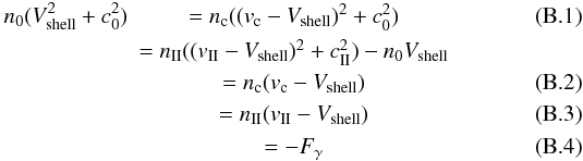 with
Fγ the ionisation flux at the I-front
(taking in account the recombination in the ionised gas). These relations are local and
we neglect the curvature of the fronts, besides the shell is assumed stationary in the
referential of the cold gas. Since the shock is strongly supersonic, the second equation
can be approximated by
with
Fγ the ionisation flux at the I-front
(taking in account the recombination in the ionised gas). These relations are local and
we neglect the curvature of the fronts, besides the shell is assumed stationary in the
referential of the cold gas. Since the shock is strongly supersonic, the second equation
can be approximated by 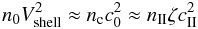 (B.5)with
ζ = 2 for a D-critical I-front
(Vshell − vII =
cII) and ζ varies from 2 to 1 in the weak
D phase. The time-scale of the expansion of the shell is much longer than the ionisation
time-scale, therefore the equilibrium between ionisation and recombination holds during
the expansion
(B.5)with
ζ = 2 for a D-critical I-front
(Vshell − vII =
cII) and ζ varies from 2 to 1 in the weak
D phase. The time-scale of the expansion of the shell is much longer than the ionisation
time-scale, therefore the equilibrium between ionisation and recombination holds during
the expansion
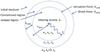 |
Fig. B.1
Outline of the collect and collapse scenario with the different variables used in the analytical model. |
| Open with DEXTER | |
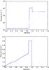 |
Fig. B.2
Density and velocity profile of a 1D spherical simulation of the ionization of a homogeneous medium in the conditions of RCW 36. The radius is between 0 and 1.5 pc with 2000 cells. The initial density is 3.4 × 104 cm-3, the ionizing flux 6 × 1047 ph s-1 and the simulation is run during 720 ky. |
| Open with DEXTER | |
 (B.6)with
Rs the Strömgren radius at the end of the R-type phase and
rshell the position of the shell at a
time t in the D-type phase. Therefore from Eqs. (B.5) and (B.6), we get
(B.6)with
Rs the Strömgren radius at the end of the R-type phase and
rshell the position of the shell at a
time t in the D-type phase. Therefore from Eqs. (B.5) and (B.6), we get 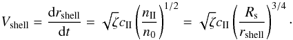 (B.7)By integration we
get the position of the shell and we set ζ to 1 (weak D-type I-front)
to get back the result from Spitzer (1978)
(B.7)By integration we
get the position of the shell and we set ζ to 1 (weak D-type I-front)
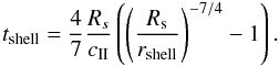
to get back the result from Spitzer (1978) 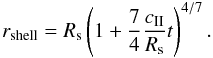 (B.8)This is the quickest
way to obtain the position of the shell that was obtained by Spitzer
(1978). The age of the H ii region can be deduced from
(B.8)This is the quickest
way to obtain the position of the shell that was obtained by Spitzer
(1978). The age of the H ii region can be deduced from
 (B.9)The density in
the shell nc can be obtained with Eq. (B.5)
(B.9)The density in
the shell nc can be obtained with Eq. (B.5)
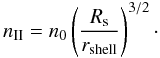
 (B.10)and
the density in the H ii region
(B.10)and
the density in the H ii region
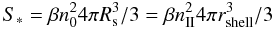
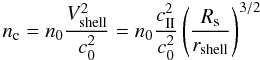
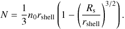
 (B.11)It is interesting
to note that the compression decreases with time. The column density N
in the shell is equal to what has been accumulated during the collect phase:
n0rshell/3 minus what remains
in the H ii region:
nIIrshell/3
(B.11)It is interesting
to note that the compression decreases with time. The column density N
in the shell is equal to what has been accumulated during the collect phase:
n0rshell/3 minus what remains
in the H ii region:
nIIrshell/3
 (B.12)The thickness of the
shell Lshell is then given by
N/nc
(B.12)The thickness of the
shell Lshell is then given by
N/nc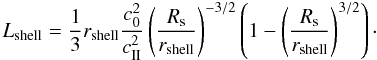 (B.13)\newpage\noindentThis
expression only depends on the shell radius and the Strömgren radius. Thus the shell
thickness and radius can be used to infer the initial Strömgren radius and the initial
density in the medium. For a shell thickness of 0.1 pc and a shell radius of 0.9 pc, the
initial H i density of the medium is 3.4 × 104 cm-3.
All the other parameters can be deduced from this density
(B.13)\newpage\noindentThis
expression only depends on the shell radius and the Strömgren radius. Thus the shell
thickness and radius can be used to infer the initial Strömgren radius and the initial
density in the medium. For a shell thickness of 0.1 pc and a shell radius of 0.9 pc, the
initial H i density of the medium is 3.4 × 104 cm-3.
All the other parameters can be deduced from this density
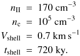 (B.14)We
compared these results with a one-dimensional spherical simulation performed with the
Heracles code (radius between 0 and 1.5 pc with 2000 cells). We took an initial density
at 3.4 × 104 cm-3, a flux of
6 × 1047 ph s-1 and run the simulation during 720 ky to reach
the observed shell radius of 0.9 pc. The density and velocity profiles are given in Fig.
B.2. In the simulation, the averaged ionised-gas
density is 170 cm-3, the compressed gas density
1.1 × 105 cm-3, the shell velocity 0.61 km s-1, and
the shell thickness 0.11 pc. The results from our simple analytical approach and the
simulation are in a good agreement (no more than 10% difference).
(B.14)We
compared these results with a one-dimensional spherical simulation performed with the
Heracles code (radius between 0 and 1.5 pc with 2000 cells). We took an initial density
at 3.4 × 104 cm-3, a flux of
6 × 1047 ph s-1 and run the simulation during 720 ky to reach
the observed shell radius of 0.9 pc. The density and velocity profiles are given in Fig.
B.2. In the simulation, the averaged ionised-gas
density is 170 cm-3, the compressed gas density
1.1 × 105 cm-3, the shell velocity 0.61 km s-1, and
the shell thickness 0.11 pc. The results from our simple analytical approach and the
simulation are in a good agreement (no more than 10% difference).
© ESO, 2013
Current usage metrics show cumulative count of Article Views (full-text article views including HTML views, PDF and ePub downloads, according to the available data) and Abstracts Views on Vision4Press platform.
Data correspond to usage on the plateform after 2015. The current usage metrics is available 48-96 hours after online publication and is updated daily on week days.
Initial download of the metrics may take a while.