| Issue |
A&A
Volume 549, January 2013
|
|
|---|---|---|
| Article Number | A74 | |
| Number of page(s) | 15 | |
| Section | Stellar structure and evolution | |
| DOI | https://doi.org/10.1051/0004-6361/201220211 | |
| Published online | 21 December 2012 | |
Seismic diagnostics for transport of angular momentum in stars
I. Rotational splittings from the pre-main sequence to the red-giant branch
1
Georg-August-Universität Göttingen, Institut für Astrophysik,
Friedrich-Hund-Platz 1,
37077
Göttingen, Germany
e-mail: jmarques@astro.physik.uni-goettingen.de
2
Observatoire de Paris, LESIA, CNRS UMR 8109,
92195
Meudon,
France
3
Observatoire de Paris, GEPI, CNRS UMR 8111,
92195
Meudon,
France
4
Institut de Physique de Rennes, Université de Rennes 1, CNRS UMR
6251, 35042
Rennes,
France
5
Département de Physique, Université de Montréal,
Montréal PQ
H3C 3J7,
Canada
6
LUPM – UM2/CNRS UMR 5299, Place Eugène Bataillon cc72, 34095
Montpellier,
France
7
Institut d’Astrophysique, Géophysique et Océanographie de
l’Université de Liège, Allée du 6
Août 17, 4000
Liège,
Belgium
8
Departamento de Astrofísica, Centro de Astrobiología
(INTA-CSIC), PO Box
78, 28691
Villanueva de la Cañada,
Madrid,
Spain
9
Laboratoire Lagrange, UMR 7293, CNRS, Observatoire de la Côte
d’Azur, Université de Nice Sophia-Antipolis, Nice, France
10
Laboratoire AIM Paris-Saclay, CEA/DSM-CNRS-Université Paris
Diderot, IRFU/SAp Centre de
Saclay, 91191
Gif-sur-Yvette,
France
11
Observatoire de Paris, LUTH, CNRS UMR 8102,
92195
Meudon,
France
Received:
13
August
2012
Accepted:
15
October
2012
Context. Rotational splittings are currently measured for several main sequence stars and a large number of red giants with the space mission Kepler. This will provide stringent constraints on rotation profiles.
Aims. Our aim is to obtain seismic constraints on the internal transport and surface loss of the angular momentum of oscillating solar-like stars. To this end, we study the evolution of rotational splittings from the pre-main sequence to the red-giant branch for stochastically excited oscillation modes.
Methods. We modified the evolutionary code CESAM2K to take rotationally induced transport in radiative zones into account. Linear rotational splittings were computed for a sequence of 1.3 M⊙ models. Rotation profiles were derived from our evolutionary models and eigenfunctions from linear adiabatic oscillation calculations.
Results. We find that transport by meridional circulation and shear turbulence yields far too high a core rotation rate for red-giant models compared with recent seismic observations. We discuss several uncertainties in the physical description of stars that could have an impact on the rotation profiles. For instance, we find that the Goldreich-Schubert-Fricke instability does not extract enough angular momentum from the core to account for the discrepancy. In contrast, an increase of the horizontal turbulent viscosity by 2 orders of magnitude is able to significantly decrease the central rotation rate on the red-giant branch.
Conclusions. Our results indicate that it is possible that the prescription for the horizontal turbulent viscosity largely underestimates its actual value or else a mechanism not included in current stellar models of low mass stars is needed to slow down the rotation in the radiative core of red-giant stars.
Key words: stars: evolution / stars: interiors / stars: rotation / stars: oscillations
© ESO, 2012
1. Introduction
Stars rotate, and this rotation has important consequences on their evolution. On the one hand, centrifugal acceleration reduces local gravity, mimicking a lower mass. On the other hand, rotation induces meridional circulation (Eddington 1925; Mestel 1953) and shear and baroclinic instabilities (Mathis et al. 2004), which contribute to the mixing of chemical elements.
The problem of transport of angular momentum inside stars has not yet been fully understood. Several mechanisms seem to be active, the most commonly invoked being diffusion by turbulent viscosity, transport by meridional circulation (Zahn 1992; Maeder & Zahn 1998), torques due to magnetic fields (Maeder & Meynet 2004; Mathis & Zahn 2005; Strugarek et al. 2011), and transport by gravity waves (Talon & Charbonnel 2005). For stars with significant convective envelopes (M⋆ ≲ 1.4 M⊙), the problem is complicated further by the magnetic braking by stellar winds (Kawaler 1988). Another problem concerns the initial rotation state, which can have an influence on the rotation profile during the pre-main sequence (PMS) and early main sequence (MS). The initial rotation state depends on the presence and lifetime of a circumstellar disk during the first stages of the PMS; magnetic fields seem to effectively lock the stellar surface to the disk (Shu et al. 1994). Maeder’s (2009) textbook contains an extensive description of these processes.
Several stellar evolutionary codes already include transport of angular momentum and associated chemical element mixing (Chaboyer et al. 1995; Talon et al. 1997; Palacios et al. 2003; Eggenberger et al. 2008). They have been developed first with a focus on studying consequences on the evolution of massive stars or evolved stars (see, e.g., Maeder & Meynet 2000; Sills & Pinsonneault 2000). The Sun and solar-like stars have been studied as above (e.g., Chaboyer et al. 1995; Zahn et al. 1997; Talon 1997), and one important application was the lithium surface depletion (e.g., Talon & Charbonnel 1998; Charbonnel & Talon 1999).
One way to study the internal transport and evolution of angular momentum is to obtain seismic information on the internal rotation profile of stars in the low and intermediate mass range at different stages of evolution. The SoHO satellite for the Sun (Turck-Chièze et al. 2010) and the ultra high precision photometry (UHP) asteroseismic space missions CoRoT (Baglin 2003) and Kepler (Borucki et al. 2010) offer such an opportunity. Seismic information has being obtained for PMS and MS stars (e.g., Benomar et al. 2010; Escobar et al. 2012), and now we also have seismic observational constraints on the internal rotation of red-giant stars (e.g., Beck et al. 2012; Mosser et al. 2012a; Deheuvels et al. 2012).
Our goal is to use seismic diagnostics to test the description of transport of angular momentum processes in 1D stellar models of low-mass stars, from the PMS to the red-giant branch (RGB). Rotational splittings (differences between nonaxisymmetric oscillation modes) are such diagnostics. When the rotation is slow, the relation between rotational splittings and rotation rate is linear and therefore relatively easy to interpret.
The information that rotational splittings provide on the internal rotation, however, depends on the physical nature of the stochastically excited modes, which in turn depend on the structure of the star, hence its age. In addition, some rotation gradient is expected to develop during the evolution; the core rotation rate is expected to become higher than the surface, as the core contracts and the envelope expands. If the rotation rate of some layers becomes too high, the associated distortion of the star and/or the Coriolis acceleration invalidates the linear approximation that provides the usual (linear) rotational splittings. In such cases, nonperturbative methods must be used (such as those developed in Lignières et al. 2006; Reese et al. 2006; Ouazzani et al. 2012). It is therefore necessary to determine if linear splitting are valid for an evolutionary stage in order to interpret correctly the observations.
We have thus started a series of papers devoted to establish seismically validated processes of transport of angular momentum that play an essential role in shaping the rotation profile of stars. The present paper is the first of this series. The second and the third will focus specifically on the case of red-giant stars. They will investigate the seismic diagnostics of rotation for slowly rotating red-giant stars for which linear rotational splittings are valid, and then rapidly rotating red-giant stars with nonperturbative methods.
In the present paper, we compute the rotation profiles and their evolution with time from the PMS to the RGB with an evolutionary code where rotationally induced mixing using the prescription of Zahn (1992) as refined by Maeder & Zahn (1998) has been implemented. We then follow the evolution of the linear rotational splittings calculated with the rotation profiles obtained from our evolutionary models and discuss their validity.
The paper is organized as follows: in Sect. 2 we describe the physical inputs that are implemented in our evolutionary code, with special emphasis on the transport of angular momentum and rotation induced mixing. We developed a version CESAM2K of the code CESAM (Morel 1997; Morel & Lebreton 2008) by implementing rotation-induced transport in radiative zones with careful attention to conservation and transport of angular momentum. The numerical scheme for the rotationally induced transport had to be modified compared to the general scheme used in CESAM2K, and some differences in the physical inputs also exist. For these reasons, the modified version will be referred to as the CESTAM code hereafter. This will avoid any possible confusion with results from other versions of CESAM2K used in the international community. The acronym CESAM stands for Code d’Evolution Stellaire Adaptatif et Modulaire, and the extra T in CESTAM stands for transport. A validated standard version of CESTAM will be made freely available.
The numerical implementation is described in Sect. 3. We then show comparisons with other codes for validation (Sect. 4). During the implementation of the code, we encountered some difficulties already present but not clearly explained in previous work. We chose to describe them carefully. In Sect. 5 we follow the evolution of theoretical linear rotational splittings for a 1.3 M⊙ sequence of stellar models evolved from the PMS to the RGB. The ℓ = 1,2 modes are computed with the ADIPLS code (Christensen-Dalsgaard 2008) in a frequency range where the modes are expected to be stochastically excited. We discuss the behavior of the splittings with frequency that can be observed during the various phases of evolution. For red-giant models, we find rotational splittings that are much higher than observed. In Sect. 6 we consider possible reasons for this disagreement. Finally, conclusions and some perspectives are given in Sect. 7.
2. Physical input
The original version of the CESAM2K code (Morel 1997; Morel & Lebreton 2008) consists of a set of routines that calculates 1D quasi-hydrostatic stellar evolution including microscopic diffusion of chemical species. The solution of the quasi-static equilibrium is performed by a collocation method based on piecewise polynomial approximations projected on a B-spline basis. For models without diffusion, the evolution of the chemical composition is solved by stiffly stable schemes of orders up to four; in the convection zones mixing and evolution of chemicals are simultaneous. The solution of the diffusion equation employs the Galerkin finite elements scheme, and the mixing of chemicals in convective zones is then performed by a strong turbulent diffusion.
The code CESAM2K allows the choice of several options for the physics. The microscopic input physics is updated regularly. The opacity tables are presently the OPAL95 data (Iglesias & Rogers 1996) complemented at low temperatures by the Wichita opacity data (Ferguson et al. 2005). Several sets of opacity tables are provided that correspond to various mixtures of chemical elements, for instance the Grevesse & Noels (1993) or Asplund et al. (2005, 2009) solar mixtures, as well as α-element enhanced mixtures. We included Pothekhin’s updated conductive opacities (see e.g. Cassisi et al. 2007). Several options are possible for the equation of state, the most commonly used being the OPAL2005 EoS (Rogers et al. 1996; Rogers & Nayfonov 2002). Several networks of nuclear reactions (and corresponding updated nuclear reaction rates) were implemented, allowing the evolution of stars to be calculated from the PMS up to helium burning. The microscopic diffusion of chemical elements includes gravitational settling, thermal, and concentration diffusion terms, but no radiative accelerations. Two formalisms are available for microscopic diffusion transport (Burgers 1969; Michaud & Proffitt 1993). Also, two options are available for treating convection, the classical MLT theory of Böhm-Vitense (1958) or the Canuto et al. (1996) so-called full spectrum of turbulence. The atmospheric boundary condition is derived either from gray model atmospheres or from Kurucz ATLAS9 models (Kurucz 2005). Overshooting is an option.
Mass loss can be considered with different prescriptions. In the models presented hereafter we use the empirical mass loss rates of Reimers (1975) scaled with metallicity according to Schaller et al. (1992).
Recently, the CESAM2K code has been involved in the ESTA activities undertaken to prepare the interpretation of the seismic observations of CoRoT. Stellar models were calculated for a range of mass, chemical composition, and the evolutionary stages corresponding to CoRoT main targets and have been compared with the results of several other evolutionary codes showing a very good general agreement (Lebreton et al. 2008a,b; Montalbán et al. 2008).
CESAM2K is freely available for download, with the details in Morel & Lebreton (2008).
2.1. Transport of angular momentum
In convective zones, although there is differential rotation in latitude, the mean rotation rate at a given radius weakly depends on the radius. Therefore, it is often assumed in 1D stellar evolution codes that convective zones rotate as solid bodies (e.g. Talon et al. 1997; Meynet & Maeder 2000; Palacios et al. 2003). In extended convective zones, however, comparisons with 3D numerical simulations suggest instead a prescription of uniform specific angular momentum (e.g. Denissenkov & Tout 2000; Palacios et al. 2006). Both options can be used in CESTAM.
In a radiative zone, we used the formalism of Zahn (1992), refined in Maeder & Zahn (1998), to model the transport of angular momentum and chemical species by meridional circulation and shear-induced turbulence. In what follows, we sketch the model to make it clear exactly which equations we adopted, as several slightly different versions have been used (e.g. Zahn 1992; Talon et al. 1997; Maeder & Zahn 1998; Denissenkov & Tout 2000; Palacios et al. 2003; Mathis & Zahn 2004).
Turbulence is expected to be highly anisotropic owing to the stable stratification in
radiative zones. Turbulence would then be much stronger in the horizontal than in the
vertical direction. Thus, the hypothesis of “shellular rotation” can be used: as
differential rotation is presumably weak along isobars, it is treated as a perturbation.
All variables f can be split into a mean value over an isobar and a
perturbation (as in Zahn 1992):
 (1)where
P2(cosϑ) is the second-order Legendre
polynomial and p is the pressure. Higher order effects, included in the
formalism developed by Mathis & Zahn
(2004), are not considered here for the moment.
(1)where
P2(cosϑ) is the second-order Legendre
polynomial and p is the pressure. Higher order effects, included in the
formalism developed by Mathis & Zahn
(2004), are not considered here for the moment.
The velocity of meridional circulation can be written in a spherical coordinate system as
 (2)where
r is the mean radius of the isobar and ϑ the
colatitude. The vertical component U2 is given in
Appendix A, following Maeder & Zahn (1998). The equation of continuity in the
anelastic approximation gives then the horizontal component
V2:
(2)where
r is the mean radius of the isobar and ϑ the
colatitude. The vertical component U2 is given in
Appendix A, following Maeder & Zahn (1998). The equation of continuity in the
anelastic approximation gives then the horizontal component
V2:  (3)where
ρ is the density.
(3)where
ρ is the density.
The transport of angular momentum obeys an advection-diffusion equation:  (4)where
νV is the vertical component of the turbulent viscosity
and d/dt represents the Lagrangian time derivative.
(4)where
νV is the vertical component of the turbulent viscosity
and d/dt represents the Lagrangian time derivative.
The relative horizontal variation of the density,  , and the mean molecular weight,
 , obey
  where
Dh is the horizontal component of turbulent diffusion
discussed in Appendix B. The evolution of Λ,
Eq. (6), depends on the competition
between the advection of a mean molecular weight gradient and its destruction by the
horizontal turbulent diffusion.
where
Dh is the horizontal component of turbulent diffusion
discussed in Appendix B. The evolution of Λ,
Eq. (6), depends on the competition
between the advection of a mean molecular weight gradient and its destruction by the
horizontal turbulent diffusion.
2.2. Evolution of the chemical composition
The vertical advection of chemicals due to the large-scale meridional circulation coupled
with a strong horizontal turbulent diffusion results in a vertical diffusion process (see,
e.g. Chaboyer & Zahn 1992). The equation of
the chemical composition evolution can then be written as
![\begin{equation} \tderiv{X_i}{t} = \frac{\partial}{\partial m} \left[ \left(4 \pi r^2 \rho \right)^2 \left(\Dv + D\ind{eff} \right) \pderiv{X_i}{m} \right] + \left. \tderiv{X_i}{t} \right|_{\rm nucl} + \left. \tderiv{X_i}{t} \right|_{\rm micro} \end{equation}](/articles/aa/full_html/2013/01/aa20211-12/aa20211-12-eq25.png) (7)where
Xi is the abundance by mass of the
ith nuclear species
and DV = νV
and Deff the vertical diffusivity and the diffusion
coefficient associated with the meridional circulation; DV
and Deff are discussed in Appendix B.
(7)where
Xi is the abundance by mass of the
ith nuclear species
and DV = νV
and Deff the vertical diffusivity and the diffusion
coefficient associated with the meridional circulation; DV
and Deff are discussed in Appendix B.
A necessary condition for shear instability is the Richardson criterion as given by Talon & Zahn (1997). Another condition is that
the turbulent viscosity νV must be greater than the molecular
viscosity, ν, as expressed by the Reynolds criterion  (8)where Rec ≃ 10
is the critical Reynolds number (Schatzman et al.
2000). When condition (8) is not
satisfied we use
DV = νV = ν.
(8)where Rec ≃ 10
is the critical Reynolds number (Schatzman et al.
2000). When condition (8) is not
satisfied we use
DV = νV = ν.
2.3. Initial conditions
Stars are fully convective when they start their PMS evolution on the Hayashi track. Assuming that convective zones rotate like solid bodies, the star should have uniform angular velocity at the beginning of its evolution.
Several facts complicate this simple picture. First, Palla & Stahler (1991) showed that stars that are more massive than about 2 M⊙ are no longer fully convective when they appear on the PMS (the exact mass depends mainly on the protostellar accretion rate and deuterium abundance). Second, if during the PMS the only process slowing down stellar rotation were the magnetic braking by stellar winds mentioned above, stars would rotate much more rapidly than observed on the ZAMS. The PMS is too short for this process to slow down the star significantly. An additional process is needed during the PMS, most likely disk locking (e.g., Bouvier et al. 1997).
Young stars are most often surrounded by a circumstellar disk left over after the main accretion phase is over. The magnetic coupling between the star and the disk slows the star down (see, e.g., Shu et al. 1994), and this effect is often modeled by assuming that the stellar surface corotates with the disk at a constant angular velocity (see Bouvier et al. 1997) as long as the disk exists. Once the disk has disappeared, the star surface rotation evolves freely. This scenario is implemented in CESTAM with the disk lifetime τdisk and period Pdisk as free parameters of the model.
2.4. Magnetic braking
Stars that are less massive than about 1.4 M⊙ have
significant outer convective zones. A solar-type dynamo operates there and generates a
magnetic field. The coupling between the magnetic field and the plasma in the stellar wind
strongly brakes the rotation of the star. Kawaler (1988,
hereafter K88) proposed the following law for the loss of angular momentum
 :
:
 (9)where
Ωsat is a saturation angular velocity, above which magnetic field generation
seems to saturate. The value of Ωsat is often set at 8–14 Ω⊙ (as
in Bouvier et al. 1997). There are indications,
however, that Ωsat varies with stellar mass (see, e.g. Krishnamurthi et al. 1997; Andronov
et al. 2003).
(9)where
Ωsat is a saturation angular velocity, above which magnetic field generation
seems to saturate. The value of Ωsat is often set at 8–14 Ω⊙ (as
in Bouvier et al. 1997). There are indications,
however, that Ωsat varies with stellar mass (see, e.g. Krishnamurthi et al. 1997; Andronov
et al. 2003).
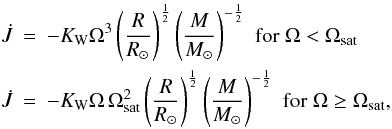
The parameter KW in Eq. (9) is usually calibrated by requiring that calibrated solar models have Ω = Ω⊙ = 2.86 × 10⁻⁶ rad s-1. The precise value of KW needed to spin down the Sun to its current period depends on the prescription for the transport of angular momentum adopted (see Sect. 4.2 below). The parameter KW should also depend on stellar mass (see, e.g. Krishnamurthi et al. 1997).
Recently, Reiners & Mohanty (2012, hereafter
RM12) have criticized the approach used in K88. Specifically, K88 supposed that
the surface magnetic flux goes as some power of the angular velocity, whereas RM12 suggest
instead that it is the magnetic field strength that obeys such a law. As a consequence,
they obtain the following law: 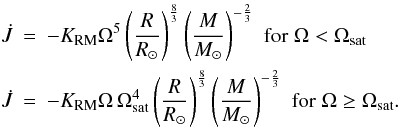 (10)The
value of KRM does not depend on the stellar mass, and
Ωsat ≃ 3 Ω⊙. Both prescriptions, Eqs. (9) and (10), are implemented in CESTAM and tested below.
(10)The
value of KRM does not depend on the stellar mass, and
Ωsat ≃ 3 Ω⊙. Both prescriptions, Eqs. (9) and (10), are implemented in CESTAM and tested below.
3. Numerical procedure
3.1. The overall problem
Stellar evolution depends on two interconnected problems: the problem of stellar structure (solving the stellar structure equations), and the problem of the evolution of the chemical composition. It has proved very difficult to solve the two problems simultaneously; different stellar evolution codes employ several techniques to overcome this difficulty. Some codes (e.g., Degl’Innocenti et al. 2008) compute the solutions of the structure equations and chemical composition in an independent way, where they use the structure calculated at the previous time step to evolve the chemical composition to the current time step, and then use this composition to calculate the structure at the current time step (or the other way around: first the structure, then the chemical composition). A second kind of code computes the chemical composition between each iteration of the structure problem, as in Scuflaire et al. (2008). And finally, Eggleton’s code (Eggleton 1971) solves the two problems simultaneously. Stancliffe (2006) has shown that differences between the three kinds of codes are only significant on the AGB.
The CESAM2K code (Morel 1997; Morel & Lebreton 2008) belongs to the second category above. It begins a time step by updating the chemical composition. With the new chemical composition, a new structure is obtained by performing one iteration of the algorithm used to solve the structure equations. This structure is used to update the chemical composition again, before a new iteration on the structure is performed. The procedure is repeated until convergence of the structure algorithm. CESTAM keeps this iterative scheme.
Rotation with angular momentum transport introduces a new problem interconnected with the previous two. The evolution of the chemical composition depends on the turbulent mixing induced by differential rotation, whereas the structure equations are changed by the inclusion of the centrifugal acceleration. In CESTAM, we inserted the resolution of the angular momentum transport equations at the beginning of the cycle, because the rotation profile is required to calculate the turbulent diffusion coefficients that are needed to update the chemical composition. Our cycle, then, is as follows: we update the rotation profile, then the chemical composition, and finally we iterate on the structure. The cycle is repeated until convergence.
In the absence of external torques, total angular momentum is conserved. The rotation
profile obtained at this stage does not enforce angular momentum conservation, however,
because the profile Ω(m) was computed with the stellar structure obtained
in the iteration before convergence. The total angular momentum is
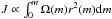 and the function
r(m) changes between iterations. We need to compute
the rotation profile one more time after convergence to make sure that it is consistent
with the stellar structure, so that angular momentum is numerically conserved.
and the function
r(m) changes between iterations. We need to compute
the rotation profile one more time after convergence to make sure that it is consistent
with the stellar structure, so that angular momentum is numerically conserved.
3.2. The rotation profile
Equation (4) (with Eqs. (A.1), (5) and (6)), is a fourth-order differential equation in r. To solve it, we split it into four first-order differential equations, and solve the system using the well known relaxation method (Henyey et al. 1964; Press et al. 2007). Equation (6) is solved simultaneously with Eq. (4), so that we have a total of five finite difference equations. We chose this method for its simplicity in dealing with the complex relations between variables expressed in Eq. (4), taking Eqs. (A.1), (5), and (6) into account. Methods that require that the solutions are approximated by a linear combination of known functions (collocation methods, spectral methods) are therefore difficult to implement. In practice, the relaxation method we employed proved to be efficient, robust, and fairly stable.
The scheme can be fully implicit or semi-implicit in time (to ensure higher order accuracy in time). The time step can be subdivided if needed, a useful feature for future developments involving faster processes.
Four boundary conditions are needed. At the top of a radiative zone, we impose
conservation of angular momentum and no differential rotation:
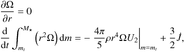 (11)where
mt is the mass inside the top of the
radiative zone. If the convective zone above it is at the surface,
(11)where
mt is the mass inside the top of the
radiative zone. If the convective zone above it is at the surface,
 is the torque applied at the surface of the star, Eq. (9), otherwise
  .
At the bottom of a radiative zone, similarly,
.
At the bottom of a radiative zone, similarly,  (12)where
mb is the mass inside the bottom of the
radiative zone. If the center of the star is radiative
(mb = 0), Eq. (12) is replaced by
U2 = 0, the requirement that there is no mass flow out of
the center.
(12)where
mb is the mass inside the bottom of the
radiative zone. If the center of the star is radiative
(mb = 0), Eq. (12) is replaced by
U2 = 0, the requirement that there is no mass flow out of
the center.
Intermediate convective regions (regions that are neither at the center nor at the
surface) are treated as if they were special points. The equations between the beginning
and the end of an intermediate convective zone (between mi and
mf) are ![\begin{eqnarray} \label{eq:conv1}&& \frac{\d}{\d t} \int_{m\ind i}^{m\ind f} \left(r^2 \Omega \right) \d m = \frac{4 \pi} 5 \left(\rho\ind i r\ind{i}^4 \Omega\ind i U\ind{2,i} - \rho\ind f r\ind{f}^4 \Omega\ind f U\ind{2,f} \right) \\[1.5mm] \label{eq:conv2}&& \left. \frac{\partial \Omega}{\partial r}\right|\ind i = 0 \\[1.5mm] \label{eq:conv3}&& \left. \frac{\partial \Omega}{\partial r}\right|\ind f = 0 \\[1.5mm] \label{eq:conv4}&& \Lambda\ind i = 0 \\[1.5mm] \label{eq:conv5}&& \Lambda\ind f = 0 . \end{eqnarray}](/articles/aa/full_html/2013/01/aa20211-12/aa20211-12-eq61.png) Equation
(13) guarantees conservation of total
angular momentum, Eqs. (14)–(15) impose no shear at the borders of the
convective zone, and Eqs. (16)–(17) result from the absence of
μ-gradients in a convective zone.
Equation
(13) guarantees conservation of total
angular momentum, Eqs. (14)–(15) impose no shear at the borders of the
convective zone, and Eqs. (16)–(17) result from the absence of
μ-gradients in a convective zone.
The four equations resulting from Eq. (4)
are written in finite-difference form between pairs of points, say, at
m = mk − 1 and
m = mk. Equation (6) requires a special treatment, because it is
not a differential equation in r (or m). We write Eq.
(6) as an algebraic equation at point
m = mk − 1, because
otherwise we would be solving for  (the average between
mk − 1 and
mk instead of the values at
mk − 1 and
mk). Indeed, Λ only appears as
in the other equations, since
it has no space derivatives. A fifth boundary condition is needed: Λ = 0 at
m = mt (the top of the
radiative zone) as in Eqs. (16)–(17).
(the average between
mk − 1 and
mk instead of the values at
mk − 1 and
mk). Indeed, Λ only appears as
in the other equations, since
it has no space derivatives. A fifth boundary condition is needed: Λ = 0 at
m = mt (the top of the
radiative zone) as in Eqs. (16)–(17).
4. Comparison with results from other evolutionary codes
The complicated nature of the equations describing the evolution of the rotation profile (and particularly the evolution of U2) made it important to validate our approach. To do that we compared our results with those obtained with other implementations of rotational mixing in stellar evolution codes, namely STAREVOL (Palacios et al. 2003) for the solar case (see also Turck-Chièze et al. 2010) and the Geneva stellar evolution code (Talon et al. 1997) for the case of 3 M⊙ and 5 M⊙ stars.
4.1. Standard physics
In these comparisons, we used the OPAL equation of state (Rogers et al. 1996) and opacities (Iglesias
& Rogers 1996), complemented
at T < 104 K by the Alexander & Ferguson (1994) opacities. We used
the NACRE nuclear reaction rates of Angulo et al.
(1999) except for the reaction, for which we used the reaction rates given in
Imbriani et al. (2004). The solar compositions of
Grevesse & Noels (1993, hereafter GN93)
and Asplund et al. (2005, hereafter AGS05) were
used. The Schwarzschild criterion was used to determine convective instability. Convective
core overshoot fully mixes the chemical composition to a distance
 from the border of the convective core (where rco is the
radius of the core determined by the Schwarzschild criterion). The temperature gradient in
the overshoot zone is ∇ = ∇ad. The centrifugal acceleration is taken into
account by adding the average centrifugal acceleration
2Ω2r/3 to gravity in the hydrostatic
equilibrium equation. The atmosphere is computed in the gray approximation and integrated
up to an optical depth of τ = 10-4.
from the border of the convective core (where rco is the
radius of the core determined by the Schwarzschild criterion). The temperature gradient in
the overshoot zone is ∇ = ∇ad. The centrifugal acceleration is taken into
account by adding the average centrifugal acceleration
2Ω2r/3 to gravity in the hydrostatic
equilibrium equation. The atmosphere is computed in the gray approximation and integrated
up to an optical depth of τ = 10-4.
Parameters of calibrated solar models.
4.2. The Sun
We computed calibrated rotating solar models using the compositions of GN93 and AGS05, with and without magnetic braking according to the magnetic braking law, Eq. (9). Models were calibrated to within 10-5 in luminosity, radius, and surface metallicity (Z = 0.0195 for GN93, Z = 0.0126 for AGS05). Initial rotational velocities (and parameter KW for the models with magnetic braking) were chosen so that models have an equatorial velocity veq = 2.02 km s-1 at the solar age (4.6 Gyr).
The temperature gradient in convective zones was computed using the convection model of Canuto et al. (1996) with l = αCGMHP. All models include microscopic diffusion and settling using the approximations proposed by Michaud & Proffitt (1993). The initial rotational velocities for the cases with braking were chosen in order to have veq = 20 km s-1 at the ZAMS.
Table 1 shows the values of parameters resulting from the solar calibration in αCGM, the initial helium, and metallicity abundances (Yi and Zi). The greatest differences between the cases with and without magnetic braking concern the initial abundances. This is because models with braking rotate much faster at the center (as shown in Turck-Chièze et al. 2010) and thus have a higher Ω-gradient, leading to a much higher turbulent diffusion. Turbulent diffusion tends to homogenize the radiative zone to a large extent, partially erasing the composition gradient created by gravitational settling.
Table 2 shows some characteristics of the calibrated solar models. The higher turbulent diffusion partially stops the settling of helium, causing a higher helium abundance in the convective zone. However, the strong Ω-gradient predicted by models with braking in the radiative zone is in direct contradiction with helioseismic results, which indicate a flat rotation profile to within r ≃ 0.25 R⊙ of the center (see, e.g. Chaplin et al. 1999; Couvidat et al. 2003; Eff-Darwich et al. 2008). A new physical mechanism is needed to explain the discrepancy, such as transport of angular momentum by internal gravity waves (see Talon & Charbonnel 2005) and/or magnetic stresses (Maeder & Meynet 2004; Mathis & Zahn 2005).
Characteristics of calibrated solar models.
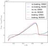 |
Fig. 1 Differences in sound speed profiles between the seismic models of Turck-Chièze et al. (2001) and CESTAM. |
Figure 1 shows differences between the sound speed cs profiles of the seismic Sun of Turck-Chièze et al. (2001) using results from SoHO (GOLF-MDI) and our calibrated solar models (see also Goupil et al. 2011, for intermediate opacities AGS09). The seismic Sun of Turck-Chièze et al. (2001) agrees with Basu et al. (2009) using results from BiSON and MDI. A good agreement at the level of 0.3% is seen when using the old mixture of GN93 with only small discrepancies below the convection zone and in the central region. On the other hand, severe discrepancies occur when more recent mixtures are used, such as AGS05. These results are quite similar to what is found in the literature (see, e.g., Basu et al. 1997; Basu & Antia 2008; Turck-Chièze et al. 2011,for models with no rotation induced transport).
We compared our results for calibrated solar models including rotation-induced transport of Type I with the results obtained in Turck-Chièze et al. (2010) with the STAREVOL code. We found good agreement between the profiles of the angular velocity, U2, and the two components of turbulent viscosity. Several improvements have been implemented in the code CESTAM compared to the CESAM2K version used in Turck-Chièze et al. (2010), but with no consequence for the solar case. We confirm that rotation induced transport of Type I does not help remove the discrepancies, as found by Turck-Chièze et al. (2010).
4.3. Higher mass, main sequence stellar models
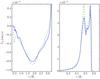 |
Fig. 2 Profiles of the vertical component of the meridional circulation U2(r) as a function of normalized radius (r/R⊙) for 5 M⊙ stellar models computed with CESTAM (continuous line) and the Geneva code (dashed line) when the central hydrogen abundance is Xc = 0.35 (see text). The left panel shows the central regions, the right panel the surface. |
We compared results for models with higher mass stars. These stars have thin convective or fully radiative surface layers and are therefore not expected to undergo magnetic braking. Calculations here are carried out assuming global conservation of angular momentum, which is obtained at the precision level of 10-6.
The first comparison concerns the evolution of a 5 M⊙ model computed with CESTAM and Geneva codes (as in Talon et al. 1997), using Xi = 0.73 and Zi = 0.01 (and no magnetic braking). These models were computed without microscopic diffusion and settling. Figure 2 shows the profile of U2(r) at the middle of the MS (when Xc = 0.35). Curves for the same quantities superimpose, showing excellent agreement between the results obtained with the two codes. There are small differences that we attribute to the different microphysics used in the codes. The rotation profiles, not shown, also agree during the course of the evolution.
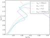 |
Fig. 3 Evolutionary tracks on the HRD for a 3 M⊙ model calculated with CESTAM code assuming either no extra mixing (dashed) or rotation with an initial equatorial velocity veq = 150 km s-1 at the ZAMS (continuous line) or without rotation but with overshooting and αov = 0.1 (dot-dashed line) and αov = 0.2 (dotted line). |
We also compared the effects of rotational mixing on the evolutionary tracks on the Herzsprung-Russel diagram (HRD) between CESTAM models and those of Eggenberger et al. (2010) computed with the Geneva code (Eggenberger et al. 2008). Figure 3 shows evolutionary tracks on the HRD for a 3 M⊙ model calculated without extra mixing (microscopic diffusion, convective overshoot, rotation), with rotational mixing only and with overshooting only.
We considered two cases for the models with overshooting, αov = 0.1 and αov = 0.2. The model with rotational mixing has veq = 150 km s-1 at the ZAMS. As in Eggenberger et al. (2010), the evolution of the rotating model closely resembles the evolution with αov = 0.1. The difference between the rotating models and the nonrotating models at the ZAMS is due to the centrifugal acceleration. The decrease in the effective gravity (gravity minus centrifugal force) replicates a nonrotating star with a lower mass.
The evolutionary tracks shown in Fig. 3 are identical to those in Fig. 2 of Eggenberger et al. (2010).
4.4. Evolved low-mass models
The rotation profiles that we obtain for our red-giant models are similar to those computed by Eggenberger et al. (2010). Examples for M⋆ = 1.3 M⊙ are given in the section below.
5. Evolution of rotational splittings from PMS to RGB
Rotational splittings are useful as seismic diagnostics for measuring the stellar internal
rotational profile. For slow rotation, a first order perturbation description provides
rotational splittings that are linearly dependent on the rotation profile. They are
therefore convenient tools, easy to compute from stellar models and theoretical oscillation
codes for comparison with observations. The first order approximation provides the following
expression for the linear rotational splittings (Christensen-Dalsgaard & Berthomieu 1991, and references therein):
 (18)where
x = r/R⋆
is the normalized radius, Ω is the angular rotation (rad/s) and the rotational kernel
Knℓ takes the form
(18)where
x = r/R⋆
is the normalized radius, Ω is the angular rotation (rad/s) and the rotational kernel
Knℓ takes the form
![\begin{equation} K_{n\ell} =\frac{1}{I_{n\ell}}~ \Bigl[\xi_r^2+\ell(\ell+1) \xi_h^2-2 \xi_r \xi_h - \xi_h^2 \Bigr] ~\rho~x^2 , \end{equation}](/articles/aa/full_html/2013/01/aa20211-12/aa20211-12-eq113.png) (19)where
Inℓ is the mode inertia
(19)where
Inℓ is the mode inertia
![\begin{equation} I_{n\ell}= {\int_0^1 ~\Bigl[\xi_r^2+\ell(\ell+1) \xi_h^2\Bigr]~\rho~x^2~ \d x}. \end{equation}](/articles/aa/full_html/2013/01/aa20211-12/aa20211-12-eq115.png) (20)The quantities entering the
equations above are the fluid vertical and horizontal displacement eigenfunctions,
ξr and
ξh respectively, and the density
ρ. For solid-body rotation, the rotational splittings become:
(20)The quantities entering the
equations above are the fluid vertical and horizontal displacement eigenfunctions,
ξr and
ξh respectively, and the density
ρ. For solid-body rotation, the rotational splittings become:
 (21)with
![\begin{equation} \beta_{n\ell} = 1-C_{n\ell}= \frac{1}{I_{n\ell}} \int_0^1 \Bigl[\xi_r^2+\ell(\ell+1) \xi_h^2-2 \xi_r \xi_h - \xi_h^2 \Bigr] ~\rho~x^2~ \d x, \end{equation}](/articles/aa/full_html/2013/01/aa20211-12/aa20211-12-eq119.png) (22)where
Cnℓ are the Ledoux coefficients.
(22)where
Cnℓ are the Ledoux coefficients.
For asymptotic pure p-modes, Cnℓ ~ 0 and βnℓ ~ 1. For pure g-modes, Cnℓ ~ 1/ℓ(ℓ + 1) and βnℓ ~ 1−1/ℓ(ℓ + 1), i.e. βnℓ ~ 1/2 for ℓ = 1 modes.
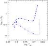 |
Fig. 4 Evolutionary track for a 1.3 M⊙ sequence of models from PMS to RGB. Dots indicate models for which rotational splittings are computed. The numbering of the selected models stars with the first dot on the PMS and ends with number 25 as the highest dot on the RGB. |
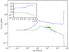 |
Fig. 5 Evolution of the central (blue line) and surface (green line) rotation rates for a 1.3 M⊙ sequence of models from the PMS to the RGB. The insert shows the central and surface rotation rates along the RGB. |
To investigate the evolution of rotational splittings with stellar age, we computed a 1.3 M⊙ evolutionary sequence including rotationally induced transport as described in Sect. 2 above. We used the same input physics as in the case AGS05 with braking described in Sect. 4.2, but without microscopic diffusion and settling, as we found that microscopic diffusion and settling do not affect the rotation profiles of our models. We chose M⋆ = 1.3 M⊙ because it is a typical seismic mass obtained for the Kepler and CoRoT red-giant stars.
Figure 4 shows an evolutionary track for a sequence of 1.3 M⊙ stellar models in a HR diagram computed with CESTAM. In order to interpret the rotational splittings, we plot the evolution of the central and surface rotation rates with age in Fig. 5.
We then computed oscillation frequencies and rotational splittings for several models spanning the track (shown in Fig. 4) using the freely available ADIPLS adiabatic oscillation code (Christensen-Dalsgaard 2008). We computed frequencies of ℓ = 0,1 axisymmetric modes and rotational splittings for ℓ = 1 modes.
The 1.3 M⊙ models have a convective envelope from PMS to
the RGB, hence we expect stochastically excited modes all along the sequence. Thus, we chose
the frequency range that spans an interval of a few radial orders below and above
nmax, the radial order corresponding to the frequency at
maximum power. It is estimated as
nmax = νmax/Δν,
where the frequency at maximum power spectrum νmax and the mean
large separation Δν are given by the usual scalings relations
 with
Teff, ⊙ = 5777 K,
νmax = 3050 μHz
and Δν⊙ = 134.7 μHz for the Sun. Indeed,
it has been conjectured, then shown observationally, that these relations predict well the
location of the excited frequency range of stochastically excited modes (e.g. Brown et al. 1991; Kjeldsen & Bedding 1995; Kallinger et al.
2010).
with
Teff, ⊙ = 5777 K,
νmax = 3050 μHz
and Δν⊙ = 134.7 μHz for the Sun. Indeed,
it has been conjectured, then shown observationally, that these relations predict well the
location of the excited frequency range of stochastically excited modes (e.g. Brown et al. 1991; Kjeldsen & Bedding 1995; Kallinger et al.
2010).
5.1. Validity of linear approximation for the rotation splittings
The validity of the linear approximation is estimated by comparing the rotation rate to
the oscillation frequency. In a perturbative approach, the parameter  (25)is
thus assumed smaller than unity. We evaluate this parameter at the center of each selected
equilibrium model of the evolutionary sequence, where Ω is largest, and for a range of
frequency spanning the radial order interval
(nmax − 4,nmax + 4).
(25)is
thus assumed smaller than unity. We evaluate this parameter at the center of each selected
equilibrium model of the evolutionary sequence, where Ω is largest, and for a range of
frequency spanning the radial order interval
(nmax − 4,nmax + 4).
Sharp rotation gradients develop in the central layers and can also cause some departure
from the linear approximation. In the oscillation equations (see, e.g. Eqs. (34.7)–(34.12)
in Unno et al. 1989), the rotation gradient term
appears with a factor  (26)Thus, we consider that
the linear approximation is valid if
(26)Thus, we consider that
the linear approximation is valid if
 (27)where the first
inequality follows from assuming ζ < 1.
(27)where the first
inequality follows from assuming ζ < 1.
We then evaluate the quantity  (28)at
the radius wherethe rotation gradient is greatest and
for ω/2π = νmax.
Figure 6 shows both quantities, ζ
and Δ, as functions of the effective temperature of the models. Both parameters remain
much smaller than unity until the model reaches the base of the RGB. Therefore, the use of
the linear approximation for the rotational splittings can be safely used for
stochastically excited solar-type modes of low mass stars except for the fast rotating
cores of red giants.
(28)at
the radius wherethe rotation gradient is greatest and
for ω/2π = νmax.
Figure 6 shows both quantities, ζ
and Δ, as functions of the effective temperature of the models. Both parameters remain
much smaller than unity until the model reaches the base of the RGB. Therefore, the use of
the linear approximation for the rotational splittings can be safely used for
stochastically excited solar-type modes of low mass stars except for the fast rotating
cores of red giants.
 |
Fig. 6 Evolution of the parameters ζ, Eq. (25) (top) and Δ, Eq. (28) (bottom), with the effective temperature of the model along its evolution from the PMS to the RGB. To be conservative, the layer where Ω is maximum is considered for ζ and the layer where the gradient is maximum is chosen for computing Δ. For ζ, we used m = −1, since ζ is higher for prograde modes, while for Δ we considered m = 1 as no difference is found for m = −1 due to the fact that Ω ≪ ω where Δ is maximum. |
5.2. Evolution of rotational splittings of stochastically excited modes along an evolutionary track
 |
Fig. 7 Top panel: rotation profiles as a function of the normalized mass m/M⋆ for 1.3 M⊙ PMS models #1 (black), #2 (cyan), #3 (red), #4 (green), #5 (blue) and #6 (magenta) shown in Fig. 4. Second panel: rotational splittings for ℓ = 1 modes as a function of the normalized frequency ν/Δν for models #1, #3, #5 and #6 (same colors as above). Third panel: βnℓ for the same models. Bottom panel: ⟨ Ω/2π ⟩ = δνnℓ/βnℓ for the same models. The large separation Δν goes from 87.9 μHz (model #1) to 106.2 μHz (model #6). |
In the following, we discuss the information that can be retrieved from the average value throughout the star ⟨ Ω/2π ⟩ = δνnℓ/βnℓ weighted by the mode. This definition is given at fixed ℓ, and depends on the radial order n.
-
The PMS regime: on the PMS, the central and surface rotationrates are equal as long as the model is fully convective. Therotation rate remains constant in time for the duration of disklocking. When the radiative core appears, the central rotationstarts to increase due to the contraction of the central layers. Whendisk locking stops, the surface rotation rate starts increasing as thestar contracts. Figure 7 shows the rotation profilesof the selected PMS models shown in Fig. 4. Thesurface rotation rate evolves from2.84 μHz (model #1) to 3.9 μHz (model #5) while the central rotation rate increases from 11.3 μHz to 21.2 μHz. The rotational splittings for ℓ = 1 modes are computed for models #1 to #6 according to Eq. (18) and are also shown in Fig. 7. The splittings are nearly independent on radial order and increase steadily with the surface rotation rate as the model evolves along the PMS towards the ZAMS. The value of the Ledoux constant almost vanishes, and βnℓ ~ 1, because the modes are essentially pressure modes in the frequency range where they are expected to be stochastically excited. These modes have no amplitudes in the inner layers and cannot probe the rotation there. Thus the mean rotation rate ⟨ Ω ⟩ /2π corresponds essentially to the rotation averaged over the outer layers. As the rotation increases inwards in these layers, we find that ⟨ Ω ⟩ /2π = 3.8 μHz for Model #1, close to – but slightly larger than – its surface rotation rate. Model #6 is already on the MS. Its surface rotation is faster than that of younger models but its central rotation is slower. This is not seen in the corresponding splittings and the averaged rotation ⟨ Ω ⟩ /2π remains close to the surface value. Results are similar for ℓ = 2 modes (not shown).
Fig. 8 Top panel: rotation profiles as a function of the normalized mass m/M⋆ for 1.3 M⊙ MS models #6 (magenta), #7 (blue), #9 (red), #10 (green) and #11 (black) shown in Fig. 4. Second panel: rotational splittings for ℓ = 1 modes as a function of the normalized frequency ν/Δν for models #7, #9, #10 and #11 (same colors as above). Third panel: βnℓ for the same models. Bottom panel: ⟨ Ω ⟩ = δνnℓ/βnℓ for the same models. The large separation Δν goes from 97.6 μHz (model #7) to 63.2 μHz (model #11).
-
The MS regime: on the MS, the surface rotation rate decreases with age due to both braking at the surface and an increase of the stellar radius. The central rotation rate also decreases with time due to transport of angular momentum from the core to the surface. The rotation in the central regions first decreases from Model #6 to #9 and increases by roughly 60% from model #9 to #11 (Fig. 8). The excited modes are still in the frequency domain of high order p-modes and their rotational splittings reflect the surface behavior only. The splittings decrease with the surface angular velocity. At the end of the MS (model #11), the central rotation rate has already reached 15.4 μHz, while the surface rotates at a rate of 0.6 μHz: the core is rotating roughly 26 times faster than the surface. As can be seen in Fig. 8, the rotational splittings for this model yield a mean rotation ⟨ Ω ⟩ /2π = 3.8 μHz, that is 1.22 μHz higher than the surface rotation rate but much lower than the central rotation rate.
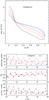
Fig. 9 Top panel: rotation profiles (logarithmic scale) as a function of the normalized mass m/M for 1.3 M⊙ subgiant models #12 (blue solid) to #17 (black solid) as indicated in Fig. 4. Second panel: rotational splittings for l = 1 modes as a function of the normalized frequency ν/Δν for model #12, #14, #15 and #16. Third panel: βnℓ for the same models. Bottom panel: ⟨ Ω ⟩ /2π = δνnℓ/βnℓ for the same models. The large separation Δν goes from 56.5 μHz (model #12) to 38.0 μHz (model #16).
-
The subgiant regime: when the model cools along the subgiant branch, its rotation keeps evolving differently in the inner and outer parts, slowing down at the surface and accelerating in the inner regions (Fig. 9). Substantial changes appear when the model leaves the MS and evolves as a subgiant. The Brunt-Väisälä frequency of red-giant stars is very high in the radiative interior, and the frequencies of g-modes enter the frequency domain of p-modes in the frequency range where stochastically excited modes are expected (Christensen-Dalsgaard 2012). During the subgiant phase, avoided crossings between p- and g-modes appear. As observationally shown (Deheuvels et al. 2010; Mosser et al. 2012b), some p-modes become mixed modes. These modes have amplitudes both in the inner regions, where they behave as gravity modes, and in the surface layers, where they behave as acoustic modes (Dziembowski & Pamyatnykh 1991). They are very interesting as they allow probing regions deep inside the star. The number of such mixed modes is small at the beginning of the subgiant branch and increases as the star evolves toward the RGB. During this phase, modes will eventually undergo avoided crossings, exchanging nature from p to g. Figure 9 shows that Model #12 is not evolved enough so that no mixed modes are present in the frequency domain shown. The splittings remain nearly frequency independent and provide a mean rotation rate close to its surface value. The variation in the splittings with frequency for the more evolved models #13 to #17 clearly shows the presence of mixed modes. With amplitudes in the dense interior, mixed modes have a much stronger inertia than the neighboring p-modes (Dupret et al. 2009). For the same reason, the rotational splittings exhibit the same behavior as the mode inertia although in a more pronounced way. They vary from one mode to the next. They are also larger than for pure p-modes when the rotation increases inward within the model. For subgiant stars, only one ℓ = 1 mixed mode exists between two consecutive radial modes. This explains the saw-like aspect of the variation in the splittings with frequency. This is confirmed by the same variation in βnℓ with frequency: p-modes have βnℓ close to 1 while mixed modes have βnℓ close to 1/2. Mixed modes enter the frequency domain by the low part and one can see that βnℓ is closer to 1 at high frequency where the g nature of the mixed modes is less pronounced. Because of the weighting by the eigenfunction, the values of the splittings yield a mean rotation ⟨ Ω ⟩ /2π that is no longer dominated by the outer layer contribution, since the mixed modes have amplitudes in the central region where the rotation rate is larger. As a result, one obtains a rotation rate that is higher than the surface value but still much lower than the rotation rate of the central regions.
-
The RGB: when the outer convective region progresses inward, its uniform rotation extends deeper as well. The surface rotation rate decreases with time essentially due to an increase in the stellar radius. The core accelerates, and in the intermediate region, where the H-burning shell lies, a sharp rotation gradient develops (see Palacios et al. 2006). The frequency spectrum of red giants is composed of g-dominated mixed modes and mixed modes with nearly equal p and g character. When the star evolves up the red-giant branch, the number of g-dominated modes increases and largely outnumbers the p-g mixed modes (Dupret et al. 2009). These modes mostly probe the core rotation (Beck et al. 2012; Deheuvels et al. 2012; Mosser et al. 2012a). For model #25 (the last shown in Fig. 4), the core rotation amounts to 251 μHz and the expected excited frequencies are about 90 μHz. This indicates a ratio ζ = 5.6 (Eq. (25)). At such rotation rates, the first-order perturbation is not relevant to computing the rotational splittings. Nonperturbative methods must then be used. However, observations show that several RGB stars have core rotation rates that are much lower than predicted by our models. (Mosser et al. 2012a). Indeed the observed values amount to a few hundred nHz, whereas here we find several dozen to a few hundred μHz. This leads to the conclusion that the central regions of our models rotate too fast and that rotationally induced transport of the kind included in our models is not efficient enough to slow down the central rotation of red-giant stars.
6. Seismic tests of transport of angular momentum: slowing down the rotating core of red-giant stars
As in the solar case, one can wonder whether another mechanism, such as internal gravity waves or magnetic fields, operates more efficiently to shape the rotation profile, either at the red-giant phase or before. However, several issues must be discussed before we can reach such a conclusion.
6.1. Uncertainties on stellar modeling and transport of angular momentum
A possible reason for this discrepancy is some inaccuracy in the current physical description of stellar models. Indeed several assumptions enter the rotationally induced transport as prescribed by Zahn (1992) and Maeder & Zahn (1998). Besides, several other uncertainties on the input physics of stellar models can also affect the resulting rotation profile to some extent. In what follows, we discuss the sensitivity of the rotation profile of red-giant models to several uncertainties.
6.1.1. Effect of convective overshoot
A 1.3 M⊙ star has a convective core during the MS. Overshoot shifts the tracks on the HR diagram, imitating tracks with higher masses. As a result, at a given radius in the RGB, the core of the model with overshoot has had less time to spin up, since it started its contraction later in the evolution. An overshoot of 0.1 HP reduces the core rotation rate by about 32% when R⋆ = 3.73 R⊙.
On the other hand, we need to reduce the mass of the model with overshoot by 0.04 M⊙ to reproduce the RGB at the same location in the HR diagram. In that case, the model with overshoot and M⋆ = 1.26 M⊙ has a central rotation rate (again, when R⋆ = 3.73 R⊙) that is similar to the central rotation rate of the model without overshoot and M⋆ = 1.3 M⊙.
6.1.2. Effect of the initial rotation state
It is well known that, after the early stages on the MS, the surface rotation rate does not depend on the initial conditions; it only depends on the magnetic braking law (Eqs. (9) and (10); see, e.g. Maeder 2009 and references therein). We found that it is indeed the case for our models. The internal rotation profile down to the center is also independent of the initial conditions after the early stages of the MS.
6.1.3. Impact of the magnetic braking law
We computed an evolution with the braking law of K88 with a value of KW twice the solar calibrated value to reduce the rotation rate. We found that the surface rotation rate is slowed down, as expected, but the central rotation rate changes only slightly. For instance, at the TAMS, the surface rotation rate changes by 20%, and by 3% at the base of the RGB, while the central rotation rate changes by 2% at the TAMS, 3% at the base of the RGB.
We calculated another evolutionary sequence with the RM12 magnetic braking law. With a coefficient KRM calibrated so as to yield the solar rotation rate in a solar model, our 1.3 M⊙ is much more efficiently slowed down compared to the evolution computed with K88. The central rotation rate, however, changes by at most 2%.
6.1.4. Stability of the rotation profile
The changes on the surface rotation rate caused by the mechanisms described above do
not change the central rotation rate significantly because the extraction of angular
momentum from the core is not efficient enough. The core and the surface are not
sufficiently coupled. One potential way of coupling the core to the surface is through
instabilities that might arise because of rotation gradient becoming very steep (as seen
in Fig. 10). The Rayleigh criterion requires that
r2Ω increases outwards. For
our 1.3 M⊙ model, the rotation profile becomes
unstable according to the Rayleigh criterion in two places, at the shell source and just
below the convective envelope. However, the stabilizing effect of the density
stratification overcomes this instability, as expressed by the Solberg-Hoiland
criterion:  (29)where
 is the
Rayleigh frequency in a rotating medium, given at the equator by
is the
Rayleigh frequency in a rotating medium, given at the equator by
 (30)According to
the Solberg-Hoiland criterion, the rotation profiles we obtain are stable throughout the
evolution. However, the Goldreich-Schubert-Fricke instability (GSF, see Goldreich & Schubert 1967; Fricke 1968) may occur in stellar conditions. Hirschi & Maeder (2010) have studied its
effects on pre-supernova models and find that if
(30)According to
the Solberg-Hoiland criterion, the rotation profiles we obtain are stable throughout the
evolution. However, the Goldreich-Schubert-Fricke instability (GSF, see Goldreich & Schubert 1967; Fricke 1968) may occur in stellar conditions. Hirschi & Maeder (2010) have studied its
effects on pre-supernova models and find that if  the
GSF instability is always present regardless of the μ− and
T − gradients. We implemented their prescription in CESTAM. Where
, turbulent transport by the
GSF instability operates with a viscosity coefficient given by the solution of their Eq.
(20),
the
GSF instability is always present regardless of the μ− and
T − gradients. We implemented their prescription in CESTAM. Where
, turbulent transport by the
GSF instability operates with a viscosity coefficient given by the solution of their Eq.
(20), ![\begin{eqnarray} \left(N^2_T + N^2_{\mu} + N^2_{\Omega}\right) x^2 &+& \left[N^2_T \Dh + N^2_{\mu} \left(K + \Dh \right) + N^2_{\Omega} \left(K + 2\Dh \right) \right]x\nonumber \\ &+& N^2_{\Omega} \left(\Dh K + \Dh^2 \right) = 0, \end{eqnarray}](/articles/aa/full_html/2013/01/aa20211-12/aa20211-12-eq192.png) (31)where
K is the thermal diffusivity given by Eq. (A.7). The viscosity coefficient associated
to the GSF instability is then given by
DGSF = 2x.
(31)where
K is the thermal diffusivity given by Eq. (A.7). The viscosity coefficient associated
to the GSF instability is then given by
DGSF = 2x.
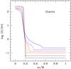 |
Fig. 10 Rotation profiles as a function of the normalized mass m/M⋆ for 1.3 M⊙ models #18 to #21 and #23, #25 (from blue to black) on the RGB as indicated in Fig. 4. |
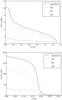 |
Fig. 11 Top: rotation profiles for 1.3 M⊙ models at the end of the MS calculated assuming standard viscosity coefficients (standard), a vertical turbulent viscosity DV computed with Ric = 1 (Ric), a horizontal viscosity coefficient 100 times the standard value (Dh), and all of the above (All). Bottom: the same for models at the base of the RGB when R⋆ = 3.73 R⊙ (Δν = 21.3 μHz). |
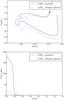 |
Fig. 12 Top: HR diagram showing the evolutionary track of a 1.2 M⊙ model computed with an overshoot of 0.1HP, a vertical turbulent viscosity DV computed with Ric = 1, a Dh increased by a factor 102 (red line, dashed), and a 1.3 M⊙ model computed without overshooting and with the “standard” viscosities (blue line, full). Dots indicate the location of models with Δν = 23.3 μHz. Bottom: rotation profiles for the models above. |
We found that in
two regions from the end of the MS, just below the border of the outer CZ and at the
shell source. At the shell source, the Ω-gradient is high because of the contraction of
the layers left behind by the movement of the shell source, while the descending CZ
lowers Ω just above its border. In our models, the GSF turbulent viscosity is on the
order of DV in the unstable regions. The
turbulent transport by the GSF instability reduces the Ω-gradient in the unstable region
at the shell source, reducing the central rotation rate by 3% in models at the base of
the RGB. The turbulent transport by the GSF instability does not have time to change the
Ω-gradient below the CZ before the convective instability sweeps over this region.
6.1.5. Uncertainties on the turbulent viscosity coefficients
To extract more angular momentum, we can either increase the meridional circulation or increase the vertical turbulent viscosity. To increase the meridional circulation, one option is to decrease the inhibiting effect of Λ (see the expression for the μ-currents, Eq. (A.5)). According to Eq. (6), an increase in Dh will lead to a decrease in Λ. The prescription for the horizontal coefficient of turbulence Dh is still open to discussion. Prescriptions derived by Zahn (1992), Maeder (2003), and Mathis et al. (2004) can differ by as much as two orders of magnitude. We adopted, as a test, a value of Dh that is 102 higher than that previously used (Eq. (B.2)).
The value of the critical Richardson number in Eq. (B.4) is usually assumed to lie between 1/4 and 1/6. Brüggen & Hillebrandt (2001) and Canuto (2002) indicate, however, that we can expect instability for Ri ≃ 1. To increase the efficiency of the vertical turbulent viscosity in transporting angular momentum from the core, we computed an evolutionary sequence using Ric = 1 to test the effect of the uncertainties. Figure 11 shows profiles of the rotation rate computed with different assumptions of the diffusion coefficients, at the TAMS and at the base of the RGB when R⋆ = 3.73 R⊙. Models have the same mass and radius, hence the same Δν. As expected, with an increased value of Ric from 1/6 to 1, the central rotation rate decreases by 18% at the TAMS and by 30% at the base of the RGB. With a Dh increased by two orders of magnitude (and Ric = 1/6), the central rotation rate decreases by 84% at the TAMS and the base of the RGB. When both changes are included (an increase of Ric and Dh as above), the central rotation rate is decreased by an order of magnitude, while we need a decrease of two orders of magnitude to reproduce the observed rotational splittings.
6.1.6. A slowly rotating red-giant model
We eventually computed an evolutionary sequence where we combined all effects causing a decrease in the rotation rate in the central region; an overshoot of 0.1 HP and a vertical turbulent viscosity DV computed with Ric = 1, together with Dh increased by a factor 102. This model was computed with M⋆ = 1.2 M⊙ because during the RGB the evolutionary track on the HRD of a 1.2 M⊙ computed with all these effects lies close to the evolutionary track of the 1.3 M⊙ models used as comparison. The resulting rotation profile for models at the base of the RGB with same Δν is significantly decreased in the central region with the central value Ωc = 21.5 μHz and is displayed in Fig. 12.
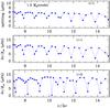 |
Fig. 13 Top: rotational splittings δνnℓ for ℓ = 1 modes as a function of the normalized frequency ν/Δν associated with the rotation profile shown in Fig. 12 for the 1.2 M⊙ model. Middle: corresponding δν/βnℓ for ℓ = 1 modes as a function of the normalized frequency ν/Δν. Bottom: the same for ℓ = 2 modes. |
Calculations of linear rotational splittings shows that the maximum splittings amounts to 5–6 μHz for model #20 at the base of the RGB (Fig. 13). This corresponds to a maximum value for δν/βnl of 12 μHz. The rotation gradient and the value of the central rotation are now too low for nonperturbative calculations to give rise to significant corrections to the values of the linear rotational splittings. Such rotation splittings lead to a core rotation rate that is closer to the observations but still too high by almost one order of magnitude compared with what is seen in recent observations (Beck et al. 2012; Deheuvels et al. 2012; Mosser et al. 2012a).
The seismology of red-giant stars emphasizes that an additional mechanism is needed to achieve a slower core rotation of red-giant stars.
7. Conclusions and perspectives
We then computed stellar evolution models of low-mass stars, taking the transport of angular momentum by turbulent viscosity and meridional circulation in radiative zones into account. As found by Palacios et al. (2006) and Eggenberger et al. (2010), the core accelerates very rapidly in our models during the subgiant and giant phases. We showed that the linear approximation for computing rotational splittings remains nevertheless valid for stochastically excited solar-type modes, for all evolutionary stages until the RGB.
For red-giant stars, interpretations of recent Kepler observations lead to a ratio between the core and surface rotation rates of five to ten, far lower than in our models where the ratio between the core and surface rotation rates approaches 103. Similar conclusions were reached by Eggenberger et al. (2012), which was published during the submission process of the present paper. Nonperturbative calculations lead to complex frequency spectra, with in particular nonsymmetric multiplets (see for instance without Coriolis force Lignières et al. 2006; Reese et al. 2006; Ouazzani et al. 2012, with both centrifugal and Coriolis force). Observations show that several red-giant stars do indeed have such complex spectra. Their core rotation is fast enough to have entangled rotational splittings and mixed-mode spacings. In such cases, rotation may have to be studied with nonperturbative methods. On the other hand, other red-giant stars (Beck et al. 2012) show frequency spectra where the rotation splittings are easily identified as symmetric patterns around axisymmetric modes. The values of the corresponding splittings are quite low, close to or smaller than 1 μHz, and using the linear approximation to derive the rotation splittings from stellar models is fully justified.
We have computed the evolution of a stellar model including rotationally induced transport taking uncertainties in the values of the parameters entering such a description into account. We achieved a decrease in the central rotation rate of a red-giant star by an order of magnitude at most, mostly due to an increase in Dh by two orders of magnitude. The modification of the parameters were chosen so as to enhance the transport of angular momentum so that the core rotation is slowed down as much as possible. The models in the red-giant phase were then slowed enough that the calculations of linear rotation splittings are valid. They were found to be one order of magnitude larger still than observed. This indicates that extraction of angular momentum from the core in our models is not efficient enough.
We need to decrease it by another order of magnitude to reproduce the observations. A similar situation is encountered in the case of the Sun. Several possibilities have been proposed, the main candidates being magnetic fields and internal gravity waves. We showed that such mechanisms must operate or keep operating during the whole subgiant and red-giant phase. In this context, Talon & Charbonnel (2008) show that transport of angular momentum by internal waves generated by the convective envelope can play an important role from the subgiant phase to the base of the RGB. They also find that this transport seems to have no major impact on stars ascending the RGB itself and later on. In the RGB phase, another mechanism must be called for to explain the observations. This will be investigated further in future work. On the observational side, measurements of rotational splittings for subgiant stars are crucially needed to constrain the efficiency for their central layers to slow down.
A standard, validated version of CESTAM will be available for download soon, together with grids of stellar models computed with several rotational velocities and adiabatic oscillation frequencies for selected models.
Acknowledgments
JPM acknowledges financial support through a 3-year CDD contract with the CNES. The authors also acknowledge financial support from the French National Research Agency (ANR) for the project ANR-07-BLAN-0226 SIROCO (SeIsmology, ROtation and COnvection with the CoRoT satellite). A.M., acknowledges the support of the Direccion General de Investigacion under project ESP2004-03855-C03-01. He also acknowledges a stay of two years at the Observatoire de Paris-Meudon.
References
- Alexander, D. R., & Ferguson, J. W. 1994, ApJ, 437, 879 [NASA ADS] [CrossRef] [Google Scholar]
- Andronov, N., Pinsonneault, M., & Sills, A. 2003, ApJ, 582, 358 [NASA ADS] [CrossRef] [Google Scholar]
- Angulo, C., Arnould, M., & the NACRE collaboration 1999, Nucl. Phys. A, 656, 3 [NASA ADS] [CrossRef] [Google Scholar]
- Asplund, M., Grevesse, N., & Sauval, A. J. 2005, in Cosmic Abundances as Records of Stellar Evolution and Nucleosynthesis, eds. T. G. Barnes, III, & F. N. Bash, ASP Conf. Ser., 336, 25 [Google Scholar]
- Asplund, M., Grevesse, N., Sauval, A. J., & Scott, P. 2009, ARA&A, 47, 481 [NASA ADS] [CrossRef] [Google Scholar]
- Baglin, A. 2003, Adv. Space Res., 31, 345 [NASA ADS] [CrossRef] [Google Scholar]
- Basu, S., & Antia, H. M. 2008, Phys. Rep., 457, 217 [NASA ADS] [CrossRef] [Google Scholar]
- Basu, S., Christensen-Dalsgaard, J., Chaplin, W. J., et al. 1997, MNRAS, 292, 243 [NASA ADS] [CrossRef] [Google Scholar]
- Basu, S., Chaplin, W. J., Elsworth, Y., New, R., & Serenelli, A. M. 2009, ApJ, 699, 1403 [NASA ADS] [CrossRef] [Google Scholar]
- Beck, P. G., Montalban, J., Kallinger, T., et al. 2012, Nature, 481, 55 [NASA ADS] [CrossRef] [Google Scholar]
- Benomar, O., Baudin, F., Marques, J. P., et al. 2010, Astron. Nachr., 331, 956 [NASA ADS] [CrossRef] [Google Scholar]
- Böhm-Vitense, E. 1958, ZAp, 46, 108 [NASA ADS] [Google Scholar]
- Borucki, W. J., Koch, D., Basri, G., et al. 2010, Science, 327, 977 [NASA ADS] [CrossRef] [PubMed] [Google Scholar]
- Bouvier, J., Forestini, M., & Allain, S. 1997, A&A, 326, 1023 [NASA ADS] [Google Scholar]
- Brown, T. M., Gilliland, R. L., Noyes, R. W., & Ramsey, L. W. 1991, ApJ, 368, 599 [NASA ADS] [CrossRef] [Google Scholar]
- Brüggen, M., & Hillebrandt, W. 2001, MNRAS, 320, 73 [NASA ADS] [CrossRef] [Google Scholar]
- Burgers, J. M. 1969, Flow Equations for Composite Gases (New York: Academic Press) [Google Scholar]
- Canuto, V. M. 2002, A&A, 384, 1119 [NASA ADS] [CrossRef] [EDP Sciences] [Google Scholar]
- Canuto, V. M., Goldman, I., & Mazzitelli, I. 1996, ApJ, 473, 550 [NASA ADS] [CrossRef] [Google Scholar]
- Cassisi, S., Potekhin, A. Y., Pietrinferni, A., Catelan, M., & Salaris, M. 2007, ApJ, 661, 1094 [NASA ADS] [CrossRef] [Google Scholar]
- Chaboyer, B., & Zahn, J.-P. 1992, A&A, 253, 173 [NASA ADS] [Google Scholar]
- Chaboyer, B., Demarque, P., & Pinsonneault, M. H. 1995, ApJ, 441, 865 [NASA ADS] [CrossRef] [Google Scholar]
- Chaplin, W. J., Christensen-Dalsgaard, J., Elsworth, Y., et al. 1999, MNRAS, 308, 405 [NASA ADS] [CrossRef] [Google Scholar]
- Charbonnel, C., & Talon, S. 1999, A&A, 351, 635 [NASA ADS] [Google Scholar]
- Christensen-Dalsgaard, J. 2008, Ap&SS, 316, 113 [NASA ADS] [CrossRef] [Google Scholar]
- Christensen-Dalsgaard, J. 2012, ASP Conf. Proc. 462, eds. H. Shibahashi, M. Takata, & A. E. Lynas-Gray, 503 [Google Scholar]
- Christensen-Dalsgaard, J., & Berthomieu, G. 1991, Theory of solar oscillations, eds. A. N. Cox, W. C. Livingston, & M. S. Matthews, 401 [Google Scholar]
- Couvidat, S., García, R. A., Turck-Chièze, S., et al. 2003, ApJ, 597, L77 [NASA ADS] [CrossRef] [Google Scholar]
- Degl’Innocenti, S., Pra da Moroni, P. G., Marconi, M., & Ruoppo, A. 2008, Ap&SS, 316, 25 [NASA ADS] [CrossRef] [Google Scholar]
- Deheuvels, S., Bruntt, H., Michel, E., et al. 2010, A&A, 515, A87 [NASA ADS] [CrossRef] [EDP Sciences] [Google Scholar]
- Deheuvels, S., García, R. A., Chaplin, W. J., et al. 2012, ApJ, 756, 19 [NASA ADS] [CrossRef] [Google Scholar]
- Denissenkov, P. A., & Tout, C. A. 2000, MNRAS, 316, 395 [NASA ADS] [CrossRef] [Google Scholar]
- Dupret, M.-A., Belkacem, K., Samadi, R., et al. 2009, A&A, 506, 57 [NASA ADS] [CrossRef] [EDP Sciences] [Google Scholar]
- Dziembowski, W. A., & Pamyatnykh, A. A. 1991, A&A, 248, L11 [NASA ADS] [Google Scholar]
- Eddington, A. S. 1925, The Observatory, 48, 73 [NASA ADS] [Google Scholar]
- Eff-Darwich, A., Korzennik, S. G., Jiménez-Reyes, S. J., & García, R. A. 2008, ApJ, 679, 1636 [NASA ADS] [CrossRef] [Google Scholar]
- Eggenberger, P., Meynet, G., Maeder, A., et al. 2008, Ap&SS, 316, 43 [NASA ADS] [CrossRef] [Google Scholar]
- Eggenberger, P., Miglio, A., Montalban, J., et al. 2010, A&A, 509, A72 [NASA ADS] [CrossRef] [EDP Sciences] [Google Scholar]
- Eggenberger, P., Montalbán, J., & Miglio, A. 2012, A&A, 544, L4 [NASA ADS] [CrossRef] [EDP Sciences] [Google Scholar]
- Eggleton, P. P. 1971, MNRAS, 151, 351 [NASA ADS] [CrossRef] [Google Scholar]
- Escobar, M. E., Théado, S., Vauclair, S., et al. 2012, A&A, 543, A96 [NASA ADS] [CrossRef] [EDP Sciences] [Google Scholar]
- Ferguson, J. W., Alexander, D. R., Allard, F., et al. 2005, ApJ, 623, 585 [NASA ADS] [CrossRef] [Google Scholar]
- Fricke, K. 1968, ZAp, 68, 317 [Google Scholar]
- Goldreich, P., & Schubert, G. 1967, ApJ, 150, 571 [NASA ADS] [CrossRef] [Google Scholar]
- Goupil, M. J., Lebreton, Y., Marques, J. P., Samadi, R., & Baudin, F. 2011, J. Phys. Conf. Ser., 271, 012031 [Google Scholar]
- Grevesse, N., & Noels, A. 1993, Phys. Scripta T, 47, 133 [Google Scholar]
- Henyey, L. G., Forbes, J. E., & Gould, N. L. 1964, ApJ, 139, 306 [NASA ADS] [CrossRef] [Google Scholar]
- Hirschi, R., & Maeder, A. 2010, A&A, 519, A16 [NASA ADS] [CrossRef] [EDP Sciences] [Google Scholar]
- Iglesias, C. A., & Rogers, F. J. 1996, ApJ, 464, 943 [NASA ADS] [CrossRef] [Google Scholar]
- Imbriani, G., Costantini, H., Formicola, A., et al. 2004, A&A, 420, 625 [NASA ADS] [CrossRef] [EDP Sciences] [Google Scholar]
- Kallinger, T., Weiss, W. W., Barban, C., et al. 2010, A&A, 509, A77 [NASA ADS] [CrossRef] [EDP Sciences] [Google Scholar]
- Kawaler, S. D. 1988, ApJ, 333, 236 [NASA ADS] [CrossRef] [Google Scholar]
- Kippenhahn, R., & Weigert, A. 1991, Stellar Structure and Evolution (Springer-Verlag) [Google Scholar]
- Kjeldsen, H., & Bedding, T. R. 1995, A&A, 293, 87 [NASA ADS] [Google Scholar]
- Krishnamurthi, A., Pinsonneault, M. H., Barnes, S., & Sofia, S. 1997, ApJ, 480, 303 [NASA ADS] [CrossRef] [Google Scholar]
- Kurucz, R. L. 2005, Mem. Soc. Astron. It. Suppl., 8, 14 [Google Scholar]
- Lebreton, Y., Montalbán, J., Christensen-Dalsgaard, J., Roxburgh, I. W., & Weiss, A. 2008a, Ap&SS, 316, 187 [NASA ADS] [CrossRef] [Google Scholar]
- Lebreton, Y., Monteiro, M. J. P. F. G., Montalbán, J., et al. 2008b, Ap&SS, 316, 1 [Google Scholar]
- Lignières, F., Rieutord, M., & Reese, D. 2006, A&A, 455, 607 [NASA ADS] [CrossRef] [EDP Sciences] [Google Scholar]
- Maeder, A. 2003, A&A, 399, 263 [NASA ADS] [CrossRef] [EDP Sciences] [Google Scholar]
- Maeder, A. 2009, Physics, Formation and Evolution of Rotating Stars (Springer Verlag) [Google Scholar]
- Maeder, A., & Meynet, G. 2000, ARA&A, 38, 143 [NASA ADS] [CrossRef] [Google Scholar]
- Maeder, A., & Meynet, G. 2004, A&A, 422, 225 [NASA ADS] [CrossRef] [EDP Sciences] [Google Scholar]
- Maeder, A., & Zahn, J.-P. 1998, A&A, 334, 1000 [NASA ADS] [Google Scholar]
- Mathis, S., & Zahn, J.-P. 2004, A&A, 425, 229 [NASA ADS] [CrossRef] [EDP Sciences] [Google Scholar]
- Mathis, S., & Zahn, J.-P. 2005, A&A, 440, 653 [NASA ADS] [CrossRef] [EDP Sciences] [Google Scholar]
- Mathis, S., Palacios, A., & Zahn, J.-P. 2004, A&A, 425, 243 [NASA ADS] [CrossRef] [EDP Sciences] [Google Scholar]
- Mestel, L. 1953, MNRAS, 113, 716 [NASA ADS] [CrossRef] [Google Scholar]
- Meynet, G., & Maeder, A. 2000, A&A, 361, 101 [NASA ADS] [Google Scholar]
- Michaud, G., & Proffitt, C. R. 1993, in Inside the Stars, eds. W. W. Weiss, & A. Baglin, ASP Conf. Ser., 40, IAU Colloq., 137, 246 [Google Scholar]
- Montalbán, J., Lebreton, Y., Miglio, A., et al. 2008, Ap&SS, 316, 219 [NASA ADS] [CrossRef] [Google Scholar]
- Morel, P. 1997, A&AS, 124, 597 [NASA ADS] [CrossRef] [EDP Sciences] [MathSciNet] [PubMed] [Google Scholar]
- Morel, P., & Lebreton, Y. 2008, Ap&SS, 316, 61 [NASA ADS] [CrossRef] [MathSciNet] [Google Scholar]
- Mosser, B., Goupil, M. J., Belkacem, K., et al. 2012a, A&A, 548, A10 [NASA ADS] [CrossRef] [EDP Sciences] [Google Scholar]
- Mosser, B., Goupil, M. J., Belkacem, K., et al. 2012b, A&A, 540, A143 [NASA ADS] [CrossRef] [EDP Sciences] [Google Scholar]
- Ouazzani, R.-M., Dupret, M.-A., & Reese, D. 2012, A&A, 547, A75 [NASA ADS] [CrossRef] [EDP Sciences] [Google Scholar]
- Palacios, A., Talon, S., Charbonnel, C., & Forestini, M. 2003, A&A, 399, 603 [NASA ADS] [CrossRef] [EDP Sciences] [Google Scholar]
- Palacios, A., Charbonnel, C., Talon, S., & Siess, L. 2006, A&A, 453, 261 [NASA ADS] [CrossRef] [EDP Sciences] [Google Scholar]
- Palla, F., & Stahler, S. W. 1991, ApJ, 375, 288 [NASA ADS] [CrossRef] [Google Scholar]
- Press, W. H., Teukolsky, S. A., Vetterling, W. T., & Flannery, B. P. 2007, Numerical Recipes, The Art of Scientific Computing, 3rd edn. (Cambridge University Press) [Google Scholar]
- Reese, D., Lignières, F., & Rieutord, M. 2006, A&A, 455, 621 [NASA ADS] [CrossRef] [EDP Sciences] [Google Scholar]
- Reimers, D. 1975, Mem. Soc. Roy. Sci. Liège, 8, 369 [Google Scholar]
- Reiners, A., & Mohanty, S. 2012, ApJ, 746, 43 [NASA ADS] [CrossRef] [Google Scholar]
- Richard, D., & Zahn, J. 1999, A&A, 347, 734 [NASA ADS] [Google Scholar]
- Rogers, F. J., & Nayfonov, A. 2002, ApJ, 576, 1064 [Google Scholar]
- Rogers, F. J., Swenson, F. J., & Iglesias, C. A. 1996, ApJ, 456, 902 [NASA ADS] [CrossRef] [Google Scholar]
- Schaller, G., Schaerer, D., Meynet, G., & Maeder, A. 1992, A&AS, 96, 269 [Google Scholar]
- Schatzman, E., Zahn, J.-P., & Morel, P. 2000, A&A, 364, 876 [NASA ADS] [Google Scholar]
- Scuflaire, R., Théado, S., Montalbán, J., et al. 2008, Ap&SS, 316, 83 [NASA ADS] [CrossRef] [Google Scholar]
- Shu, F., Najita, J., Ostriker, E., et al. 1994, ApJ, 429, 781 [NASA ADS] [CrossRef] [Google Scholar]
- Sills, A., & Pinsonneault, M. H. 2000, ApJ, 540, 489 [NASA ADS] [CrossRef] [Google Scholar]
- Stancliffe, R. J. 2006, MNRAS, 370, 1817 [NASA ADS] [CrossRef] [Google Scholar]
- Strugarek, A., Brun, A. S., & Zahn, J.-P. 2011, A&A, 532, A34 [NASA ADS] [CrossRef] [EDP Sciences] [Google Scholar]
- Talon, S. 1997, Ph.D. Thesis, Observatoire de Paris, 187 [Google Scholar]
- Talon, S., & Charbonnel, C. 1998, A&A, 335, 959 [NASA ADS] [Google Scholar]
- Talon, S., & Charbonnel, C. 2005, A&A, 440, 981 [NASA ADS] [CrossRef] [EDP Sciences] [Google Scholar]
- Talon, S., & Charbonnel, C. 2008, A&A, 482, 597 [NASA ADS] [CrossRef] [EDP Sciences] [Google Scholar]
- Talon, S., & Zahn, J.-P. 1997, A&A, 317, 749 [Google Scholar]
- Talon, S., Zahn, J.-P., Maeder, A., & Meynet, G. 1997, A&A, 322, 209 [NASA ADS] [Google Scholar]
- Turck-Chièze, S., Couvidat, S., Kosovichev, A. G., et al. 2001, ApJ, 555, L69 [NASA ADS] [CrossRef] [Google Scholar]
- Turck-Chièze, S., Palacios, A., Marques, J. P., & Nghiem, P. A. P. 2010, ApJ, 715, 1539 [NASA ADS] [CrossRef] [Google Scholar]
- Turck-Chièze, S., Piau, L., & Couvidat, S. 2011, ApJ, 731, L29 [NASA ADS] [CrossRef] [Google Scholar]
- Unno, W., Osaki, Y., Ando, H., Saio, H., & Shibahashi, H. 1989, Nonradial oscillations of stars, 2nd edn. (Tokyo: University of Tokyo Press) [Google Scholar]
- Zahn, J.-P. 1992, A&A, 265, 115 [NASA ADS] [Google Scholar]
- Zahn, J.-P., Talon, S., & Matias, J. 1997, A&A, 322, 320 [Google Scholar]
Appendix A: meridional circulation
The vertical component of the meridional circulation is given by ![\appendix \setcounter{section}{1} \begin{eqnarray} \label{eq:u2} U_2 &=& \frac{p}{c_p \rho T g \left[\nabla_{\rm ad} - \nabla + (\varphi/\delta) \nabla_{\mu} \right]} \nonumber \\[3mm] &&\times \left[\frac{L_r}{M^{\star}} \left(E_{\Omega} + E_{\mu} \right) + \frac{c_p T}{\delta} \frac{\d \Theta}{\d t} \right], \end{eqnarray}](/articles/aa/full_html/2013/01/aa20211-12/aa20211-12-eq219.png) (A.1)where
cp,T,g,∇, and
∇ad have their usual meanings (as defined in Kippenhahn & Weigert 1991). In Eq. (A.1) above, M ⋆ is the
reduced mass,
(A.1)where
cp,T,g,∇, and
∇ad have their usual meanings (as defined in Kippenhahn & Weigert 1991). In Eq. (A.1) above, M ⋆ is the
reduced mass, 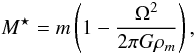 (A.2)where m
and ρm are the mass and mean density inside
an isobar, respectively, and EΩ
and Eμ denote the so-called Ω-
and μ-currents (following Palacios
et al. 2003). The quantities ϕ and δ are
obtained from the equation of state, and are defined as in Kippenhahn & Weigert (1991),
(A.2)where m
and ρm are the mass and mean density inside
an isobar, respectively, and EΩ
and Eμ denote the so-called Ω-
and μ-currents (following Palacios
et al. 2003). The quantities ϕ and δ are
obtained from the equation of state, and are defined as in Kippenhahn & Weigert (1991),
 (A.3)The Ω- and
μ-currents are given by
(A.3)The Ω- and
μ-currents are given by ![\appendix \setcounter{section}{1} \begin{eqnarray} E_{\Omega} &=& 2 \left(1 - \frac{\Omega^2}{2 \pi G \rho} - \frac{\bar{\varepsilon} + \bar{\varepsilon}_g}{\varepsilon_m} \right) \frac{\tilde{g}} {\bar{g}} \nonumber \\ && - \frac{\rho_m}{\rho} \left\{ \frac{r}{3} \frac{\partial}{\partial r} \left[H_T \frac{\partial}{\partial r}\left(\frac{\Theta}{\delta} \right) - \chi_T \frac{\Theta}{\delta} + \left(1 - \frac{1}{\delta} \right) \Theta \right] \right . \nonumber \\ && \left . - \frac{2 H_T}{r}\left(1 + \frac{\Dh}{K} \right)\frac{\Theta}{\delta} + \frac 2 3 \Theta \right\} \nonumber \\ && - \frac{\bar{\varepsilon} + \bar{\varepsilon}_g}{\varepsilon_m} \left[H_T \frac{\partial}{\partial r} \left( \frac{\Theta}{\delta} \right) + \left(f_{\varepsilon} \varepsilon_T - \chi_T \right) \frac{\Theta}{\delta} \right. \nonumber \\ && \left. + \left(2 - f_{\varepsilon} - \frac{1}{\delta} \right)\Theta \right] \label{eq:eomega} \\ E_{\mu} &=& \frac{\rho_m}{\rho} \left\{\frac{r}{3} \frac{\partial}{\partial r} \left[H_T \frac{\partial}{\partial r} \left(\frac{\varphi}{\delta} \Lambda \right) - \left(\chi_{\mu} + \frac{\varphi}{\delta} \chi_T + \frac{\varphi}{\delta} \right)\Lambda \right] \right . \nonumber \\ && - \left . \frac{2 H_T}{r} \frac{\varphi}{\delta}\Lambda \right\} + \frac{\bar{\varepsilon} + \bar{\varepsilon}_g}{\varepsilon_m} \left\{H_T \frac{\partial}{\partial r}\left(\frac{\varphi}{\delta} \Lambda \right) \right . \nonumber \\ && \left . + \left[f_{\varepsilon} \left(\varepsilon_{\mu} + \frac{\varphi}{\delta} \varepsilon_{T} \right) - \chi_{\mu} - \frac{\varphi}{\delta}\left(\chi_T + 1 \right)\right]\Lambda \right\} \label{eq:emu}. \end{eqnarray}](/articles/aa/full_html/2013/01/aa20211-12/aa20211-12-eq230.png) In
Eqs. (A.4) and (A.5) we used the following quantities:
In
Eqs. (A.4) and (A.5) we used the following quantities:
 and
and  are the nuclear and gravitational energy generation rates,
εm = L/m
the mean energy production inside a sphere of radius r,
and ρm = 3m/(4πr3)
the mean density. The thermal conductivity χ is given by
are the nuclear and gravitational energy generation rates,
εm = L/m
the mean energy production inside a sphere of radius r,
and ρm = 3m/(4πr3)
the mean density. The thermal conductivity χ is given by
 (A.6)and the thermal
diffusivity is
(A.6)and the thermal
diffusivity is  (A.7)We also used
 (A.8)the temperature scale
height;
(A.8)the temperature scale
height;  (A.9)the logarithmic
derivatives of χ;
(A.9)the logarithmic
derivatives of χ;
 (A.10)the logarithmic
derivatives of ε; and
(A.10)the logarithmic
derivatives of ε; and
 (A.11)
Appendix B: turbulent coefficients of diffusivity
The coefficient Deff is given by (Chaboyer & Zahn 1992)
 (B.1)We use the prescription
of Mathis et al. (2004) for the horizontal
component of turbulent diffusivity Dh:
(B.1)We use the prescription
of Mathis et al. (2004) for the horizontal
component of turbulent diffusivity Dh:
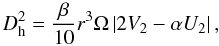 (B.2)where
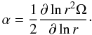 (B.3)We take the coefficient
β = 1.5 × 10⁻⁵ (Richard
& Zahn 1999).
(B.3)We take the coefficient
β = 1.5 × 10⁻⁵ (Richard
& Zahn 1999).
For the vertical component DV, we use the prescription of
Talon & Zahn (1997), 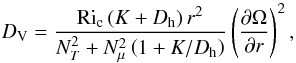 (B.4)where
Ric = 1/6 is the critical Richardson number,
K the thermal diffusivity,
NT and
Nμ the chemical and thermal parts of the
Brunt-V*error*˝ais*error*˝ala˝ frequency,
(B.4)where
Ric = 1/6 is the critical Richardson number,
K the thermal diffusivity,
NT and
Nμ the chemical and thermal parts of the
Brunt-V*error*˝ais*error*˝ala˝ frequency,  :
:
 (B.5)
(B.5)
All Tables
All Figures
|
Fig. 1 Differences in sound speed profiles between the seismic models of Turck-Chièze et al. (2001) and CESTAM. |
| In the text | |
|
Fig. 2 Profiles of the vertical component of the meridional circulation U2(r) as a function of normalized radius (r/R⊙) for 5 M⊙ stellar models computed with CESTAM (continuous line) and the Geneva code (dashed line) when the central hydrogen abundance is Xc = 0.35 (see text). The left panel shows the central regions, the right panel the surface. |
| In the text | |
|
Fig. 3 Evolutionary tracks on the HRD for a 3 M⊙ model calculated with CESTAM code assuming either no extra mixing (dashed) or rotation with an initial equatorial velocity veq = 150 km s-1 at the ZAMS (continuous line) or without rotation but with overshooting and αov = 0.1 (dot-dashed line) and αov = 0.2 (dotted line). |
| In the text | |
|
Fig. 4 Evolutionary track for a 1.3 M⊙ sequence of models from PMS to RGB. Dots indicate models for which rotational splittings are computed. The numbering of the selected models stars with the first dot on the PMS and ends with number 25 as the highest dot on the RGB. |
| In the text | |
|
Fig. 5 Evolution of the central (blue line) and surface (green line) rotation rates for a 1.3 M⊙ sequence of models from the PMS to the RGB. The insert shows the central and surface rotation rates along the RGB. |
| In the text | |
|
Fig. 6 Evolution of the parameters ζ, Eq. (25) (top) and Δ, Eq. (28) (bottom), with the effective temperature of the model along its evolution from the PMS to the RGB. To be conservative, the layer where Ω is maximum is considered for ζ and the layer where the gradient is maximum is chosen for computing Δ. For ζ, we used m = −1, since ζ is higher for prograde modes, while for Δ we considered m = 1 as no difference is found for m = −1 due to the fact that Ω ≪ ω where Δ is maximum. |
| In the text | |
|
Fig. 7 Top panel: rotation profiles as a function of the normalized mass m/M⋆ for 1.3 M⊙ PMS models #1 (black), #2 (cyan), #3 (red), #4 (green), #5 (blue) and #6 (magenta) shown in Fig. 4. Second panel: rotational splittings for ℓ = 1 modes as a function of the normalized frequency ν/Δν for models #1, #3, #5 and #6 (same colors as above). Third panel: βnℓ for the same models. Bottom panel: ⟨ Ω/2π ⟩ = δνnℓ/βnℓ for the same models. The large separation Δν goes from 87.9 μHz (model #1) to 106.2 μHz (model #6). |
| In the text | |
|
Fig. 8 Top panel: rotation profiles as a function of the normalized mass m/M⋆ for 1.3 M⊙ MS models #6 (magenta), #7 (blue), #9 (red), #10 (green) and #11 (black) shown in Fig. 4. Second panel: rotational splittings for ℓ = 1 modes as a function of the normalized frequency ν/Δν for models #7, #9, #10 and #11 (same colors as above). Third panel: βnℓ for the same models. Bottom panel: ⟨ Ω ⟩ = δνnℓ/βnℓ for the same models. The large separation Δν goes from 97.6 μHz (model #7) to 63.2 μHz (model #11). |
| In the text | |
|
Fig. 9 Top panel: rotation profiles (logarithmic scale) as a function of the normalized mass m/M for 1.3 M⊙ subgiant models #12 (blue solid) to #17 (black solid) as indicated in Fig. 4. Second panel: rotational splittings for l = 1 modes as a function of the normalized frequency ν/Δν for model #12, #14, #15 and #16. Third panel: βnℓ for the same models. Bottom panel: ⟨ Ω ⟩ /2π = δνnℓ/βnℓ for the same models. The large separation Δν goes from 56.5 μHz (model #12) to 38.0 μHz (model #16). |
| In the text | |
|
Fig. 10 Rotation profiles as a function of the normalized mass m/M⋆ for 1.3 M⊙ models #18 to #21 and #23, #25 (from blue to black) on the RGB as indicated in Fig. 4. |
| In the text | |
|
Fig. 11 Top: rotation profiles for 1.3 M⊙ models at the end of the MS calculated assuming standard viscosity coefficients (standard), a vertical turbulent viscosity DV computed with Ric = 1 (Ric), a horizontal viscosity coefficient 100 times the standard value (Dh), and all of the above (All). Bottom: the same for models at the base of the RGB when R⋆ = 3.73 R⊙ (Δν = 21.3 μHz). |
| In the text | |
|
Fig. 12 Top: HR diagram showing the evolutionary track of a 1.2 M⊙ model computed with an overshoot of 0.1HP, a vertical turbulent viscosity DV computed with Ric = 1, a Dh increased by a factor 102 (red line, dashed), and a 1.3 M⊙ model computed without overshooting and with the “standard” viscosities (blue line, full). Dots indicate the location of models with Δν = 23.3 μHz. Bottom: rotation profiles for the models above. |
| In the text | |
|
Fig. 13 Top: rotational splittings δνnℓ for ℓ = 1 modes as a function of the normalized frequency ν/Δν associated with the rotation profile shown in Fig. 12 for the 1.2 M⊙ model. Middle: corresponding δν/βnℓ for ℓ = 1 modes as a function of the normalized frequency ν/Δν. Bottom: the same for ℓ = 2 modes. |
| In the text | |
Current usage metrics show cumulative count of Article Views (full-text article views including HTML views, PDF and ePub downloads, according to the available data) and Abstracts Views on Vision4Press platform.
Data correspond to usage on the plateform after 2015. The current usage metrics is available 48-96 hours after online publication and is updated daily on week days.
Initial download of the metrics may take a while.