| Issue |
A&A
Volume 549, January 2013
|
|
|---|---|---|
| Article Number | A57 | |
| Number of page(s) | 16 | |
| Section | Galactic structure, stellar clusters and populations | |
| DOI | https://doi.org/10.1051/0004-6361/201219773 | |
| Published online | 18 December 2012 | |
Young, massive star candidates detected throughout the nuclear star cluster of the Milky Way ⋆,⋆⋆
1 National Astronomical Observatory of Japan, Mitaka, Tokyo 181-8588, Japan
e-mail: This email address is being protected from spambots. You need JavaScript enabled to view it.
2 Instituto de Astrofísica de Andalucía (CSIC), Glorieta de la Astronomía s/n, 18008 Granada, Spain
e-mail: This email address is being protected from spambots. You need JavaScript enabled to view it.
Received: 8 June 2012
Accepted: 20 October 2012
Abstract
Context. Nuclear star clusters (NSCs) are ubiquitous at the centers of galaxies. They show mixed stellar populations and the spectra of many NSCs indicate recent events of star formation. However, it is impossible to resolve external NSCs in order to examine the relevant processes. The Milky Way NSC, on the other hand, is close enough to be resolved into its individual stars and presents therefore a unique template for NSCs in general.
Aims. Young, massive stars have been found by systematic spectroscopic studies at projected distances R ≲ 0.5 pc from the supermassive black hole, Sagittarius A* (Sgr A*). In recent years, increasing evidence has been found for the presence of young, massive stars also at R > 0.5 pc. Our goal in this work is a systematic search for young, massive star candidates throughout the entire region within R ~ 2.5 pc of the black hole.
Methods. The main criterion for the photometric identification of young, massive early-type stars is the lack of CO-absorption in the spectra. We used narrow-band imaging with the near-infrared camera ISAAC at the ESO VLT under excellent seeing conditions to search for young, massive stars within ~2.5 pc of Sgr A*.
Results. We have found 63 early-type star candidates at R ≲ 2.5 pc, with an estimated erroneous identification rate of only about 20%. Considering their K-band magnitudes and interstellar extinction, they are candidates for Wolf-Rayet stars, supergiants, or early O-type stars. Of these, 31 stars are so far unknown young, massive star candidates, all of which lie at R > 0.5 pc. The surface number density profile of the young, massive star candidates can be well fit by a single power-law (∝ R−Γ), with Γ = 1.6 ± 0.17 at R < 2.5 pc, which is significantly steeper than that of the late-type giants that make up the bulk of the observable stars in the NSC. Intriguingly, this power-law is consistent with the power-law that describes the surface density of young, massive stars in the same brightness range at R ≲ 0.5 pc.
Conclusions. The finding of a significant number of newly identified early-type star candidates at the Galactic center suggests that young, massive stars can be found throughout the entire cluster which may require us to modify existing theories for star formation at the Galactic center. Follow-up studies are needed to improve the existing data and lay the foundations for a unified theory of star formation in the Milky Way’s NSC.
Key words: Galaxy: center / stars: formation / stars: early-type
Table 2 is available in electronic form at http://www.aanda.org
FITS files of the mosaic images, and tables of the photometry are only available at the CDS via anonymous ftp to cdsarc.u-strasbg.fr (130.79.128.5) or via http://cdsarc.u-strasbg.fr/viz-bin/qcat?J/A+A/549/A57
© ESO, 2012
1. Introduction
Nuclear star clusters (NSCs) are ubiquitous in galaxies and appear as compact clusters at the dynamical centers of their host galaxies (e.g., Böker et al. 2002; Carollo et al. 1998; Côté et al. 2006). They have luminosities in the range 105 − 108 L⊙, effective radii of a few pc, and masses of the order 106 − 108 M⊙. They are typically 1–2 orders of magnitude brighter and more massive than globular clusters (Walcher et al. 2005), which places NSCs among the most massive known clusters in the Universe (see Böker 2010, for a brief review on NSCs). Star formation in NSCs appears to be a (quasi-)continuous process. The majority of NSCs have mixed old and young stellar populations and show frequently signs of star formation within the past 100 Myr (e.g., Walcher et al. 2006). NSCs show complex morphologies and frequently coexist with supermassive black holes (SMBHs; Seth et al. 2006, 2008).
Sagittarius A* (Sgr A*), the SMBH at the center of the Milky Way (MW), with a mass of roughly 4 million solar masses and located at a distance of about 8 kpc (e.g., Ghez et al. 2008; Gillessen et al. 2009), is surrounded by a dense and massive star cluster, the MW’s NSC, which has an estimated mass of 3 ± 1.5 × 10⁷ M⊙ (Launhardt et al. 2002) and a half light radius of 3–5 pc (Graham & Spitler 2009; Schödel 2011, see the latter paper for a brief review on the MW NSC). The mid-infrared images from the Spitzer Space Telescope show how the NSC stands out as a separate structure at the center of the MW (Stolovy et al. 2006).
Summary of observations.
Star formation events occurred in the central parsec of the Galactic center (GC) about 108 and a few times 106 years ago (Krabbe et al. 1995). The massive, young stars formed in the most recent star formation event were found to be concentrated within a projected radius of R = 0.5 pc around the central SMBH, with their density increasing toward Sgr A*. About half of them appear to be located within a disk-like structure (Levin & Beloborodov 2003; Paumard et al. 2006; Lu et al. 2009). The currently favored hypothesis for their formation is that they formed about 6 Myr ago in situ in a dense gas disk around the SMBH (e.g., Bonnell & Rice 2008; Bartko et al. 2010). An alternative scenario for the presence of young, massive stars in the central parsec is the formation of a massive cluster at more than several parsecs distance from the SMBH, followed by its infall toward the central parsec via dynamical friction and its subsequent dissolution (e.g., Gerhard 2001; Kim & Morris 2003). However, this hypothesis encounters difficulties in explaining observations such as the steep increase of the surface density of the young stars toward Sgr A* and the relatively low total mass of the young, massive stars in the central 0.5 pc (see discussion in Bartko et al. 2010). Also, the apparent absence of X-ray radiation from young, low-mass stars in the central parsecs disfavors the cluster infall hypothesis (Nayakshin & Sunyaev 2005).
Extinction toward the central parsecs of the GC is extreme, AV = 30–50 mag and variable on arcsecond scales (e.g., Scoville et al. 2003; Schödel et al. 2010), which means that stellar colors are dominated by extinction, and broad-band colors can hardly be used to distinguish between late- and early-type stars (see, however, the carefully extinction corrected color–magnitude diagram in Fig. 8 of Schödel et al. 2010). Alternative methods to identify young, massive stars are spectroscopy, X-ray plus infrared multi-wavelength observations, search for emission lines, or near-infrared imaging with filters sensitive to the CO-absorption of late-type stars. Since spectroscopic observations are very intensive in observing time, they were almost exclusively focused toward a region within R ~ 0.5 pc from Sgr A*, with only a few observed fields at 0.5 < R < 0.8 pc (e.g., Do et al. 2009; Bartko et al. 2010). Despite of the small area examined, spectroscopic observations dominate our current understanding of star formation at the GC with the view that young, massive stars can almost exclusively been found within R ~ 0.5 pc of Sgr A*.
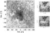 |
Fig. 1 Image of the GC through the 2.25 μm narrow-band filter of ISAAC (left). The inserts on the right show a detail after (top) and before (bottom) correction of the row bias, which removes most, but not all, of the variable detector background. |
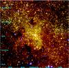 |
Fig. 2 Near-infrared three-color (1.19 μm, 1.71 μm, and 2.25 μm) composite image of the central ~ 150″ region of our Galaxy. East is to the left, and north is up. |
However, evidence for the presence of young, massive stars in the NSC at distances R > 0.5 pc from Sgr A* has been steadily increasing in the past years. Geballe et al. (2006) analyzed the spectrum of a single star, IRS 8, located about 1 pc north of Sgr A*, and identified it as a O5-O6 giant or supergiant. This source was an obvious target for dedicated spectroscopic observations because it is surrounded by a bow-shock and thus stands out from the field. Mauerhan et al. (2010b) combined X-ray and near-infrared observations to identify a few dozen Wolf-Rayet stars and O giants or supergiants throughout the central region (at R < 100 pc) of the MW. These observations are probably particularly sensitive to massive binaries, where the X-ray emission is produced in colliding winds. Wang et al. (2010), Dong et al. (2011), and Mauerhan et al. (2010a) used Pa α narrow-band imaging with HST to find young, massive stars throughout within a few tens of pc of Sgr A*. This method picks out most likely massive stars with strong winds, but it runs into problems in the central parsecs near Sgr A* because of the bright emission from the interstellar medium in the so-called mini-spiral (Ekers et al. 1983; Lo & Claussen 1983) and the relatively low angular resolution that they used (FWHM ≈ 0.2″). An efficient way of distinguishing between young, massive stars and old, late-type stars in imaging data is near-infrared imaging that makes use of the CO-absorption at λ ≈ 2.3 μm in the atmospheres of the cool stars (Genzel et al. 2003; Buchholz et al. 2009). Young, massive stars are identified in this method through the absence of CO-absorption combined with their high luminosity. Buchholz et al. (2009) used this method, combined with adaptive optics (AO) imaging and found evidence for a population of young, massive stars at R > 0.5 pc from the central SMBH. However, the use of AO with the correspondingly small instrumental field-of-view (FOV) restricted them to a relatively small region at R ≤ 20′′/0.8 pc from Sgr A*.
Here, we present the results of a systematic search for young, massive stars within R ≈ 2.5 pc of Sgr A* via imaging data from the VLT near-infrared camera ISAAC1. Our method is narrow-band seeing-limited imaging under good seeing conditions, using the CO-band absorption of late-type stars to distinguish between young, massive, early-type stars and late-type giants in the central ~6 × 6 pc. Recurrence to seeing-limited observations allow us to probe a significantly larger FOV than what would be possible in comparable time with AO imaging. Our work has some overlap with, but is also complementary to the above-mentioned work.
2. Observations and data reduction
Imaging observations were acquired through various narrow-band filters with ISAAC at the ESO VLT (Moorwood et al. 1998). The FOV is  with a pixel scale of 0
 15. Details of the observations are listed in Table 1. The angular resolution of observations with ISAAC are limited by seeing, which is of special importance here because the GC is an extremely crowded field. Note that the DIMM seeing measurements listed in Table 1 present a pessimistic over-estimation of the actual seeing values. On the one hand, according to the Roddier formula, the seeing FWHM ∝ λ-0.2, hence visual seeing of 1.0″ translates to about 0.8″ at 2.09 μm. On the other hand, the DIMM measurements on Paranal are influenced by a turbulent layer close to the ground that hardly affects the telescopes themselves (Sarazin et al. 2008). The average point-source FWHM in all our images is therefore only about 0.5″−0.6″.
Most of the data reduction process was standard, with sky subtraction, bad pixel correction, and flat-fielding. The sky observations were acquired with identical settings as the target observations, but on a dark cloud about 713′′ west and 400′′ north of Sgr A*.
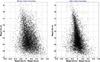 |
Fig. 3 [2.25] vs. [2.25] − [2.34] color magnitude diagrams before (left) and after (right) the color correction. See Sect. 3.2 in detail. |
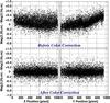 |
Fig. 4 Color dependence of point sources along the x- and y-axes on the infrared array. We can see a clear color trend before the color correction (upper panels). However, after the correction (bottom panels), no clear dependence can be seen. See Sect. 3.2 in detail. |
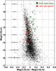 |
Fig. 5 [2.25] vs. [2.25] − [2.34] color magnitude diagram after the color correction and the elimination of sources with large photometric uncertainties. Known early-type stars and late-type giants are marked by green circles and red triangles, respectively. |
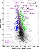 |
Fig. 6 [2.25] vs. [2.25] − [2.34] color magnitude diagram. Red color (positive value) in [2.25] − [2.34] means no significant CO absorption at 2.34 μm which, together with the brightness, is an indicator for massive, early-type stars. Typical uncertainties are represented by grey crosses at the left side. Stars with photometric uncertainties larger than these typical ones are not included in this diagram. The reddening vector with a slope of Aλ ∝ λ-2.0 (Nishiyama et al. 2006) is shown at the upper right in the diagram. Dark green circles represent spectroscopically identified early-type stars. The means and sigmas of the RGB in the [2.25] − [2.34] color within bins of one magnitude width are shown by pink circles and bars, respectively. We define stars more than 2-σ redder than the red giants as early-type star candidates (light green crosses). Blue crosses, which are stars more than 2-σbluer than the RGB, are used to estimate the false detection likelihood of the early-type star candidates. |
A non-standard part of the image reduction process was taking care of detector row bias variations as described in the Instrument Data Reduction Cookbook, issue 80.0, edited by ESO Paranal Science Operations and available on the ESO web site. Since different rows of the detector are read out at different times when applying double correlated read, different parts of the detector sample different parts of the non-linear integration ramp. This can lead to important biases for short integration times and bright sources. The bias variations depend on integration time and detector illumination, and are not constant in time. In particular, the bias depends on the brightness and distribution of sources over the FOV and is therefore different for each pointing. The bias variations are non-uniform across the detector and cannot be modeled by a smoothly varying function. Since the upper and lower halves of the detector are read out in parallel there is a visible jump of the background around detector row 512 in individual exposures.
However, the bias variations are largely restricted to the vertical (y-)direction on the detector and the bias is, to 0th order, uniform along each row. Therefore, the bias can, in principle, be reliably determined by measuring the median along each row, after suitably clipping the highest and lowest pixel values. A difficulty in this procedure is that the GC is extremely crowded and there are hardly any pixels on the detector that do not contain part of the PSF of a star. After some experimenting we chose to use the median of the 200 lowest pixels from each row to estimate the bias. The 200 lowest pixels usually fall on dark clouds in almost each row in each image, where the bias can then be determined with reasonable accuracy, but at the price of losing information on the absolute background emission. After bias correction the images were combined into a final mosaic.
The 2.25 μm narrow-band image is shown in Fig. 1, along with zooms onto a detail in the final mosaics composed from the bias-corrected and from the uncorrected images. The procedure for bias correction worked well, but some systematic errors remained, particularly because the brightness and density of stars is highly non-uniform across the images, which leads to over-estimation of the bias in rows crossing the center of the cluster and under-estimation of the bias in rows that cross dark patches of strong extinction. Since the final mosaics were composed of dithered images, the systematic errors of the bias correction were somewhat smeared across the final mosaics. Since we used PSF fitting for photometry, with a simultaneous estimation of the background, the impact of a variable background on photometry is somewhat mitigated. Nevertheless, as discussed below, we could observe color trends in our data, mainly along the y-direction, with a jump near the middle of the images. We believe that these color trends are related to the uncertainties of the bias correction. A near-infrared three-color (1.19 μm, 1.71 μm, and 2.25 μm) composite image of the central ~150″ region is shown in Fig. 2.
3. Data analysis
3.1. Photometry
We performed source detection and point-spread function (PSF) fitting with the IRAF (Imaging Reduction and Analysis Facility)2 and DAOPHOT packages (Stetson 1987). We used the daofind task to identify point sources, and the sources were then input for PSF fitting photometry to the allstar task. The PSF model was constructed using a “Penny1” function3. From 50 to 100 sources were used to construct the variable PSF for each image. The PSF model was linearly variable over the image with terms proportional to pixel offsets in the x- and y-directions.
The photometric calibration was carried out using a photometric catalog of point sources (Schödel et al. 2010). In the catalog, H-, KS-, and L′-band magnitudes of point sources in the central 40″ × 40″ region are listed. The PSF-fitting magnitudes for the NB1.71 filter were calibrated with the H-band magnitudes, and those in the NB2.09, NB2.25, NB2.34 bands were calibrated with the KS magnitudes. The small bias introduced by this procedure among the NB2.09, NB2.25, and NB2.34 bands could be neglected for our purpose because we are primarily interested in differential photometry, where overall offsets are of little importance. In the following, we search for early-type stars by using the magnitude difference between the NB2.25 and NB2.34 bands.
An astrometric calibration was done using the IRSF/SIRIUS point source catalog by Nishiyama et al. (2006). Positions of point sources in this catalog were calibrated with the 2MASS point source catalog (Skrutskie et al. 2006), and the positional accuracy of the IRSF/SIRIUS catalog was estimated to be ~0.1″. Due to image distortion, differences between stellar positions in the IRSF/SIRIUS catalog and ISAAC images are as large as 0.3″ at the corners of the images, although the differences at the image center are within 0.1″. This astrometric calibration was done in order for matching of our sources with other observations. The matches in stellar positions were calculated automatically at first, but a confirmation of the matching was done by eye, by plotting the position of the matched sources on the ISAAC images.
To avoid spurious detections of point-like sources, the sources were used in the following analysis only if a source was detected in all of the five observations of the NB2.09, NB2.25, and NB2.34 bands (see Table 1).
3.2. Color correction and source selection
Although PSF fitting was done with optimized parameters and a variable PSF, the resulting color magnitude diagram still had a large scatter (see the left panel in Fig. 3). The typical error in the [2.25] − [2.34] color4 is from 0.15 to 0.19 at [2.25] < 13.5, which is larger than the expected difference of ~0.1 mag between early-type dwarfs and late-type giants at ~2.3 μm (Buchholz et al. 2009). To investigate the cause of the large scatter, we made [2.25] − [2.34] color distribution profiles as functions of the image x- and y-axes (upper panels in Fig. 4). We can see a clear color trend along the y-axis and a discontinuity at y ≈ 500 pixel, the probable cause of which is described in the last paragraph of Sect. 2. The mean [2.25] − [2.34] color at y ~ 0 is ~−0.1, but at y ~ 950 it is about + 0.4. This trend is thus identified as the principle cause of the large scatter in the CMD. There is also a trend along the x-axis, but it is continuous and has a smaller amplitude.
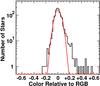 |
Fig. 7 Histogram of stellar colors relative to the RGB mean (pink circles in Fig. 6). Only stars with [2.25] < 12.25 mag are used for this histogram. A Gaussian fit is shown by a red line. An excess is clearly seen on the right (redder) side of the RGB, indicating the existence of early-type stars in this region. |
To improve the CMD, we carried out a color correction to reduce the influence of the color trend, and eliminated stars with large photometric uncertainties. For the color correction, we assumed that the average of the intrinsic stellar colors is the same throughout the observed field. This assumption is appropriate for our observed field due to similar intrinsic colors of almost all stellar types observable around the K band, the dominance of late-type giants in the GC region, and the restricted wavelength range of our observations. This assumption is also well justified in the case of GC, and has been used in previous work, e.g., Schödel et al. (2007, 2010), where this point is further discussed and illustrated.
At first, to correct the color trend along the y-axis, the observed field was divided into sub-fields of 1024 (x) × 20 (y) pixels. The [2.25] − [2.34] color histograms of stars in the sub-fields were constructed and fit with Gaussian functions. As described above, the intrinsic colors of the histograms’ peaks are expected to be almost the same, and the difference between the central wavelengths of the NB2.25 and NB2.34 filters is only 0.09 μm. Preliminary color-shifts for each sub-field were therefore calculated by requiring that the peak of each Gaussian had a color of [2.25] − [2.34] = 0. After the color-shifts along the y-axis we carried out a similar procedure along the x-axis, by dividing the observed field into sub-fields of 20 (x) × 1024 (y) pixels. The [2.25] − [2.34] color distribution profiles after the color correction are shown in Fig. 4, bottom panels. After correction there appears to be no significant color trend along either the x- or the y-axis. The CMD after the color correction is shown in the right panel in Fig. 3.
Next, stars with large photometric uncertainties were eliminated from our source list. The stellar density is extreme in the GC, which means that a large fraction of sources will indeed be affected by systematic photometric errors due to source confusion. Comparing two images taken under different seeing conditions is an efficient way of identifying and excluding those sources from our sample. Since two independent sets of observations existed for the NB2.25 and NB2.34 bands (see Table 1), we could estimate the photometric uncertainties of the stars from the differences between these two measurements. We calculated the rms of the photometric uncertainties in bins of one magnitude width, and eliminated stars with uncertainties larger than the rms. Through this procedure, 3063 sources out of 8014 were excluded from our source list. The final CMD with 4951 sources is shown in Fig. 5. The typical combined uncertainties of the [2.25] − [2.34] color (squared sum of the photometric uncertainties in both bands) now range from 0.06 to 0.08 at [2.25] < 13.5, more than a factor of two smaller than those without the color correction and the elimination of the sources with large photometric uncertainties.
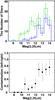 |
Fig. 8 Top: magnitude histograms for early-type star candidates (green) and stars more than 2-σbluer than the RGB (see Fig. 6). This shows that the number of stars at the redder side (earlier spectral type) of the RGB is clearly larger than that at the bluer side (later spectral type). Bottom: ratio of the bluer stars to the early-type star candidates. If we assume that the bluer stars are red giants with a large photometric uncertainty, a similar number of stars may contaminate our sample of the early-type star candidates. So this diagram shows the expected ratio of such contamination for the candidates. The uncertainties in the top panel are given by the square root of the counts in each bin. For stars brighter than [2.25] = 12.25 mag, the contamination is low (≲ 25%). |
3.3. Source classification
The final CMD has sufficient photometric accuracy to differentiate early-type stars from late-type giants. In Fig. 5, we show the [2.25] − [2.34] CMD, in which spectroscopically confirmed late-type giants (Maness et al. 2007) and early-type stars (Paumard et al. 2006, Table B.1) are marked by red squares and green circles, respectively. The majority of sources in our final sample lie on a sequence from ([2.25] − [2.34] , [2.25]) ~ (−0.2,9.5) to (0.1,15.5). This coincides with the location of most of the spectroscopically identified giants, indicating that the sequence is the red giant branch (RGB) on this CMD. On the other hand, at [2.25] ≲ 12.5, most of the known early-type stars (green circles) are located to the right of the RGB, and only two of a total of 23 early-type stars lie on the RGB. Red color in [2.25] − [2.34] means no significant CO absorption at 2.34 μm, thus suggesting an early spectral type. Hence Fig. 5 reveals that early-type stars can be identified reliably in our sample at [2.25] ≲ 12.5. From the location of the spectroscopically identified stars, we estimate a probability of false identifications on the order of 10% in this region of the CMD.
To automatically identify early-type stars and to determine the magnitude limit of our procedure, we proceeded as follows. We constructed [2.25] − [2.34] color histograms for stars within one magnitude wide bins in [2.25] , and fit the histograms with Gaussian functions. The mean and standard deviation, σ, of the best fit for each bin are shown by pink circles and pink bars in Fig. 6, respectively. The mean and σ correspond to the mean color and width of the RGB in each magnitude bin. We defined stars more than 2σ redder than (i.e., to the right of) the mean RGB color as early-type star candidates (light green crosses in Fig. 6).
The color histograms of the RGB are expected to follow a normal distribution. When we construct a histogram of a “relative” [2.25] − [2.34] color from the mean of the RGB, the histogram shows a normal distribution of the RGB plus an excess component of the early-type stars at the red side of the histogram (Fig. 7). So the “blue” stars, which are the blue tail of the normal distribution of the RGB, can be used to estimate the contamination of the early-type star candidates by RGB stars because of measurement errors. So we define stars more than 2σbluer than the RGB as “blue” stars (blue crosses in Fig. 6).
Magnitude histograms of the early-type candidates and the “blue” stars are shown in Fig. 8, top panel. The number of blue stars is very small at [2.25] < 12.25, but it increases at [2.25] > 12.25. The bottom panel in Fig. 8 shows the ratio of the blue stars to the early-type candidates, i.e., the expected contamination of the early-type candidates by erroneous identification. The ratios are less than ~ 25% at [2.25] < 12.25, and more than 60% at [2.25] > 12.25. Therefore we can conclude that the magnitude limit above which we can differentiate the early-type star candidates from the red giants is [2.25] ≈ 12.25. The stars with [2.25] < 9.75 are also excluded from the candidates due to unreliable photometry caused by detector saturation.
In the magnitude range of 9.75 < [2.25] < 12.25, we have found 63 early-type star candidates. In the same magnitude range, 20 spectroscopically confirmed early-type stars are included in the final CMD (green circles in Figs. 5 and 6, from Schödel et al. 2009, Table B.1). Of these, only one source is mis-identified as a red giant, and the others are recognized as early-type stars in our analysis.
In the same magnitude range, we have found 12 “blue” stars located at the left side of the RGB. Assuming that the “blue” stars are red giants with a large photometric uncertainty, and the number of falsely identified early-type candidates is similar, the probability of contamination is estimated to be 12/63 = 0.19. However, as described below, 5 of the 63 candidates are not early-type stars, but intrinsically very red sources. By assuming that these two sources of uncertainty are independent, this increases the estimated contamination of early-type candidates to 21%. Note that this is a conservative estimate because the very red sources could be excluded by an additional color cut. This would, however, complicate our analysis unnecessarily. Also, some of these sources are probably early-type stars that are surrounded by bow-shocks (Tanner et al. 2005).
3.4. [2.25] vs. [1.71] – [2.25] CMD
We constructed an extinction-corrected [2.25] vs. [1.71] − [2.25] CMD (Fig. 9) which is expected to be very similar to a broad band K vs. H − K CMD. For the data sets of the NB1.71 and NB2.25 filter, we did the same procedure of the color correction and the elimination of the sources with large photometric uncertainties as described in Sect. 3.2. Then, we carried out “relative” extinction correction following the procedure in Schödel et al. (2010); we calculated the mean of the [1.71] − [2.25] colors of the 10 nearest stars, ([1.71] − [2.25])mean, at each position, and the mean color excess E [1.71] − [2.25] = ([1.71] − [2.25])mean − 2.1 was used for the “relative” extinction correction of the sources in the NB1.71 and NB2.25 bands. Here we assume that most of the nearest stars are late-type red giants which have a mean color of [1.71] − [2.25] = 2.1 at the GC. More than 1-mag bluer ([1.71] − [2.25] < 1.1) or redder ([1.71] − [2.25] > 3.1) sources are excluded from the nearest star list because they are considered background or foreground stars.
By comparing both the [2.25] vs. [2.25] − [2.34] CMD (Fig. 6) and the [2.25] vs. [1.71] − [2.25] CMD (Fig. 9), a major benefit of the narrow-band observations with the NB2.25 and NB2.34 filters is easily understandable. In the [2.25] vs. [1.71] − [2.25] CMD, it is difficult to find a difference in the distributions between the spectroscopically confirmed early-type stars (green circles; Paumard et al. 2006; Schödel et al. 2009) and late-type giants (red triangles; Maness et al. 2007) even after our extinction correction. This means that the accuracies of the photometry and extinction correction are not sufficient to distinguish the early-type stars from the giants. On the other hand, almost all of the known early-type stars are identified as early-type star candidates in the [2.25] vs. [2.25] − [2.34] CMD at 9.75 < [2.25] < 12.25 (Fig. 6).
Although the [2.25] vs. [1.71] − [2.25] CMD is not practical for the early-type star search, it is very useful to find foreground objects because the [1.71] − [2.25] color is sensitive to the interstellar extinction. Of the early-type star candidates, only one source has a very blue color of [1.71] − [2.25] ≈ 0.7, and it is clearly a foreground object. However, the other sources have similarly red colors as the spectroscopically confirmed early-type stars and giants in the GC. They are thus likely to be located in the GC. To eliminate foreground contamination, stars with [1.71] − [2.25] < 1.5 are excluded from the following analysis.
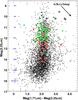 |
Fig. 9 [2.25] vs. [1.71] − [2.25] color magnitude diagram. The early-type star candidates are overplotted by light green crosses. Dark green circles and red triangles represent spectroscopically identified early-type stars and late-type giants, respectively. Most of the candidates have a [1.71] − [2.25] color (almost equivalent to a H − K color) of more than 1.5, suggesting that they suffer from strong (AK ≳ 2) extinction, and thus they are not foreground sources. |
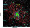 |
Fig. 10 Spatial distribution of the early-type star candidates with 9.75 < [2.25] < 12.25 (green circles) within the FOV of our observations. The candidates which have been unknown so far are indicated by blue arrows. Red giants identified by our analysis are marked by red circles. The large blue circle delimits a region within 0.5 pc (12 |
4. Results and discussion
According to the definition of the early-type star candidates described above, we have found 63 candidates in the range of 9.75 < [2.25] < 12.25 (Table 2). Considering their magnitude and the interstellar extinction of AK ~ 2−3 mag in this region, they are candidates for Wolf-Rayet stars, supergiants, or early O-type stars.
An advantage of the early-type star search with the NB2.25 and NB2.34 narrow-band filters is an almost negligible influence of interstellar extinction. The small difference (0.09 μm) of the central wavelengths of the two filters introduces a very small color excess of E [2.25] − [2.34] = 0.07AKS, according to the interstellar extinction law toward the GC (Aλ ∝ λα and α ≈ − 2.0, where Aλ is the amount of extinction at the wavelength λ; Nishiyama et al. 2006; Schödel et al. 2010). In addition, the reddening vector on the [2.25] vs. [2.25] − [2.34] CMD is almost parallel to the RGB (Fig. 6). So the objects on the CMD show shifts parallel to the RGB due to the interstellar extinction, which has thus a negligible effect on the classification of the sources.
4.1. Comparison with other observations
Intrinsically very red sources which we here call dust embedded sources (DES), exist in the central parsec of our Galaxy (e.g., Moultaka et al. 2004; Tanner et al. 2005; Geballe et al. 2006). They are included in our list of the early-type star candidates because there is good evidence that at least some of them are young, massive stars (Tanner et al. 2005). The position of the DESs on our CMD is shown in Fig. 6. With the exception of IRS 2L, all of them lie far to the right in the CMD. Several known DESs, such as IRS 1W, 9, 13, are excluded from our final source list because of insufficient photometric accuracy.
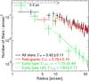 |
Fig. 11 Plots of the azimuthally averaged, stellar surface number densities as a function of projected distance from Sgr A* for all stars in our sample (black), red giants (red), and early-type star candidates (green), with 9.75 < [2.25] < 12.25. The densities were determined in annuli of variable width, chosen such that each one contained a fixed number of stars (5 stars for the early-type star candidates, and 15 stars for the entire sample and the red giants). Data points at 10″ ≤ RSgrA∗ ≤ 60″ were used for power-law fits of the radial profiles for our entire sample (black line), red giants (red line), and early-type star candidates (green line). The green dashed line represents a power-law fit to the densities of the early type candidates, including those at RSgrA∗ ≤ 10″. |
In the region we observed there are 18 sources with significant Pa α emission (the primary Pa α emitting sources in Dong et al. 2011). Since most of them are concentrated within 0.5 pc of Sgr A*, where source confusion is severe in our images, only seven sources are found to be matched with our final list (source ID 117, 121, 123, 124, 129, 131, 133 in Dong et al. 2011)5. Three sources (122, 127, 128) are not identified as point sources due to source blending, one (128) is too faint for reliable detection, and the others (38, 118, 119, 120, 125, 126, 132) are excluded from our list due to large photometric uncertainties. As shown in Fig. 6 (purple squares), all of the seven sources in our list, one of which is as faint as [2.25] ~ 14, are distributed on the right side of the RGB. It follows that our method can reliably identify young, massive stars that were found via their Pa α emission.
After excluding the DESs, we find that 20 of our early-type candidates lie within the fields observed with VLT/SINFONI (Bartko et al. 2010)6. Of those, 18 sources are confirmed as early-type stars with spectroscopic observations. This fact supports our claim that the sources distributed on the right side of the RGB on the CMD are reliable candidates for early-type stars.
Spectra of six of our early-type candidates were obtained by Blum et al. (2003), who identified four of them as hot/young stars (IRS 3, 6E, 21, 15NE) and two of them as late-type giants (see Table 2).
Twenty-eight of our early-type star candidates, after having excluded the DESs, have been previously observed with VLT/NACO and narrow-band filters (Buchholz et al. 2009). Although six of those sources were classified as late-type stars, 18 of them were listed as high quality early-type candidates. Two of the remaining sources could not be classified by Buchholz et al. (2009) because of a noisy (IRS 16SW) or strongly reddened SED (ID 480), while a further two sources are not listed in their catalog.
To summarize the comparison with past observations: we have found seven Pa α sources (Dong et al. 2011) in our source list, and all of them are identified as early-type star candidates; 20 of our candidates are included in the observed fields by Bartko et al. (2010), and 18 of them are spectroscopically classified as young, massive stars; Blum et al. (2003) observed spectroscopically six of our candidates and report four of them as early-type stars; 18 among 28 matches between our candidates and stars from the AO imaging observations by Buchholz et al. (2009) are classified as high-quality early-type star candidates in their work, and only six of the matches are classified as late-type stars. The complete list of young, massive star candidates found in our observations, along with their measured colors, is contained in Table 2.
4.2. Spatial distribution
In Fig. 10, we show the NB2.25 filter image on which we have marked the early-type star candidates (light green circles) and the stars on the RGB (red dots) with 9.75 < [2.25] < 12.25. There is a significant concentration of the early-type candidates within a projected distance RSgrA∗ of 0.5 pc from Sgr A*. These young, massive stars are well known from previous imaging and spectroscopic observations (e.g., Paumard et al. 2006; Do et al. 2009; Bartko et al. 2010). However, more than half (35) of our candidates are found at RSgrA∗ > 0.5 pc, in regions that have so far hardly been examined with spectroscopic observations. Although spectroscopic confirmation is necessary, the large number of the candidates, the small contamination probability of ~20%, and the findings by other authors (e.g., Dong et al. 2011) suggest the existence of a significant number of young, massive stars at distances R > 0.5 pc from Sgr A*.
The intrinsic distribution of young, massive stars will of course differ from the observed one because the probability of identifying a candidate at a given location depends on factors such as extinction, crowding and local PSF. The apparent lack of sources in the south eastern and north western parts of the FOV is due to extremely high extinction in these regions (see Schödel et al. 2007). Due to strong PSF distortion near the corners and edges of the FOV of our observations, the density of sources in our sample (both the red giants and early-type stars) decreases significantly toward the south-eastern, north-western, and north-eastern corners of the FOV. However, none of these difficulties affects our main finding of a significant number of so far unknown candidates for young, massive stars at projected distances between 0.5 and 3.2 pc from Sgr A*.
Azimuthally averaged, projected stellar surface density plots as a function of the distance to Sgr A* for all stars, red giants, and early-type candidates with 9.75 < [2.25] < 12.25 are shown in Fig. 11. This analysis is limited to the region within 60″ from Sgr A*, to extract stellar surface densities in full rings, and to exclude the regions with low completeness near the corners of our images. The bin widths were chosen such that each bin contains a constant number of stars (five stars for the analysis of early-type star candidates only, and 15 stars otherwise) in order to give each data point roughly the same statistical weight.
The surface density profiles show clearly that the spatial distribution of young, early-type stars is different from that of old, red giants outside the central 0.5 pc. We find an apparently continuous surface density profile for the early-type star candidates in the range  . The profile was fit with a power law (∝ R − Γ) which gives a spectral index of ΓEarly = 1.60 ± 0.17. On the other hand, the profiles of the entire sample and for the red giants show a break around 10″ (as known from previous work, e.g., Eckart et al. 1993; Schödel et al. 2007), so the fitting was carried out only in the range of 10″ ≤ RSgrA∗ ≤ 60″, providing power-law indices of Γall = 0.92 ± 0.11 and ΓRG = 0.76 ± 0.10 for all stars and red giants, respectively. For comparison, we also fit the profile for the early-type star candidates only for RSgrA∗ = 10″ to 60″, and obtain ΓEarly, > 10″ = 1.75 ± 0.49. Note that we have not made any extinction and completeness corrections for these plots, and thus the absolute values of Γ may have additional systematic errors; however, it is possible to compare the three indices, Γall, ΓRG, and ΓEarly (or ΓEarly, >10″), because they suffer almost the same interstellar extinction and have the same photometric completeness limits. Also, the power-law indices inferred here agree well with previous work (see below). The early-type star candidates show a steep, apparently continuous radial profile, while the red giants show a shallower profile with a break at ~10″. The significant difference of the profiles also suggests that not every early-type star found in our analysis is contamination by erroneous identification of a late-type giant.
While the power-law indices derived here may suffer from some additional systematic uncertainties as discussed above, those for the entire sample and the red giants, Γall = 0.92 and ΓRG = 0.76 are in good agreement with previous observations. Schödel et al. (2007) produced a fit of a broken power law to the surface number density profile of the stars in the NSC, regardless of type, and found Γ = 0.75 ± 0.10 outside a break radius at  . Through narrow-band imaging observations, Buchholz et al. (2009) obtained Γ = 0.86 ± 0.06 and 0.70 ± 0.09 for all sources and late-type stars, respectively, at 6″ ≤ RSgrA∗ ≤ 20″. Here our limiting magnitude, [2.25] = 12.25, is much shallower than K = 17.75 (Schödel et al. 2007) and K = 15.5 (Buchholz et al. 2009). So the agreement implies that incompleteness and variable extinction do not affect our result significantly within the photometric limit of this work.
Interestingly, the power-law indices for the early-type star candidates are also similar to previous results at RSgrA∗ ≲ 10″. We construct a plane-of-the-sky projected surface density plot for early-type stars with 9.75 < K < 12.25 catalogued in Bartko et al. (2009), and find ΓEarly = 1.47 ± 0.42. This is consistent, within the uncertainties, with our values of ΓEarly, >10″ = 1.75 ± 0.49, and also ΓEarly = 1.60 ± 0.17.
4.3. Implications for star formation at the Galactic center
In the central parsec, where the potential is dominated by the 4 × 10⁶ M⊙ SMBH, the densities for a molecular cloud to be stable against tidal disruption are on the order of a few 1010 (108,107) nH2 cm-3 at r = 0.1 (0.5,1.0) pc distance from Sgr A*. These extreme densities are several orders of magnitude larger than what is found in molecular clouds near the GC (see, e.g., discussion in Genzel et al. 2003). Standard in situ star formation is therefore considered to be impossible in the central parsec of the MW. Two alternative scenarios were therefore suggested to explain the presence of young, massive stars in the central parsec: (1) formation of the stars in a fragmenting gas disc or streamer around the SMBH (e.g., Nayakshin et al. 2007); (2) formation of a massive, dense stellar cluster at more than several parsecs distance and its subsequent infall and dissolution (e.g., Gerhard 2001).
The young, massive stars at the GC were found to be concentrated mainly within R ~ 0.5 pc, with the highest concentration near Sgr A* and a steep fall-off of their surface density toward larger distances. Along with some evidence for a very top-heavy initial mass function of these stars (Bartko et al. 2010, see however Do et al., in prep.) and with the absence of X-ray emission from low-mass pre main sequence stars from a potential dissolved progenitor cluster (Nayakshin & Sunyaev 2005), this appears to favor the scenario of star formation in a gaseous disk around Sgr A*.
It has to be kept in mind, however, that our current ideas on star formation at the GC are influenced by the limitations of observational studies. Those studies have been focused largely on the region within a projected radius of R ≲ 1 pc from Sgr A*. The main reason for this limitation is that spectroscopic searches are very costly and are therefore limited to small numbers of stars and/or to small areas. Therefore it is still unclear whether a clear outer edge of the distribution of the early-type stars exists or not. Recently, further spectroscopic observations found about 10 new early-type stars outside the central 0.5 pc (Bartko et al. 2010), and as described in the introduction, ever more observational results support the existence of young, massive stars at larger distances from the SMBH.
Here we present the results of the first systematic search, via narrow-band imaging, for young, massive stars within a projected distance of R ~ 2.5 pc of Sgr A*. Although our survey is limited to the brightest (K < 12.25) stars in the field because of the limited photometric accuracy imposed by the seeing-limited observations in this heavily crowded field, we detect a significant number of candidates for young, massive stars distributed throughout the studied region, with half of them located at R > 0.5 pc. The brightness range of these candidates suggests that they are of similar type – and therefore age – than the young, massive stars in the central 0.5 pc. As Fig. 10 shows, these stars appear to be randomly throughout the NSC (small number statistics keep us from studying this aspect more quantitatively). Intriguingly, a single power-law, with an exponent of Γ = 1.60 ± 0.17, can provide a good fit to the surface density of the young, massive stars as a function of distance from Sgr A* throughout the studied region. This power-law agrees within the uncertainties with the power-law that describes the surface density of correspondingly bright young stars within R = 0.5 pc of Sgr A*, that were identified in spectroscopic studies (e.g., Bartko et al. 2009).
Our finding that a single power-law can describe the surface density of early type candidates throughout the examined region may indicate a physical connection between the young, massive stars inside and outside of the central 0.5 pc. Can these stars have formed in the outer parts of the hypothetical gas disk? It seems to be difficult to form massive stars via this mechanism at r > 0.5 pc. Hobbs & Nayakshin (2009) suggest that the young stars at the GC could have been formed in a high-inclination collision of two massive gas clouds. In their simulation, gaseous streams or filaments, that extend as far out as 1 pc from Sgr A*, become self-gravitating and form stars. However, most of the stars formed in the streamers are low mass stars (0.1 − 1 M⊙), while the most massive stars are concentrated toward the central 0.5 pc region, in contrast with our observations. Mapelli et al. (2012) also show that in the outer part (r > 1 pc) of the hypothetical disk, the gas density is lower and thus the Jeans mass becomes about an order of magnitude larger than in the central few tenths of a parsec. Hence, the resultant star formation efficiency is very low outside a few tenths of a parsec. Since most of the existing theoretical work has focused on explaining the presence of young, massive stars at r < 0.5 pc, without having observational evidence for a significant population of young, massive stars at larger distances, they were not optimized to explain star formation at greater distances. Therefore, further studies are necessary to investigate whether star formation in infalling clouds/gaseous disks can explain the presence of young, massive stars beyond r ~ 1 pc as well. Also, deeper photometric studies, similar to the one described here, are needed to set tighter constraints on the statistics of young, massive stars throughout the region studied here and to confirm or reject the hypothesis that a single power-law can be applied to their surface density from 0 to 2.5 pc.
As concerns the cluster-infall scenario, our results do not significantly alter the currently accepted picture because the fundamental observation stays valid that the young, massive stars are strongly concentrated toward Sgr A*. Nevertheless, we cannot yet reliably exclude the possibility that the candidates for young, massive stars at R ≳ 1 pc may have been deposited at their current location by the dissolution of a stellar cluster at larger distances, in an event that was unrelated to the stars within R ~ 0.5 pc of Sgr A*. Gürkan & Rasio (2005), for example, showed that a ~5 × 10⁵ M⊙ stellar cluster with an initial position of 10 pc from the SMBH can sink into the central a few pc within a lifetime of young, massive stars (a few Myr). Since the surface density profiles predicted from the inspiralling cluster scenario strongly depend on models employed in simulations (see, e.g., simulations by Kim & Morris 2003; Berukoff & Hansen 2006; Fujii et al. 2010), it is difficult to exclude the cluster scenario by comparing the surface density profiles. Kinematic information of the candidates is presumably crucial to discriminate the above scenarios.
We can also consider the possibility that young, massive stars at R ≳ 1 pc were formed in a different event (or events) than the ones at R ≲ 0.5 pc. The required density of molecular clouds against tidal destruction by the tidal shear from Sgr A* is reduced to a few 106 nH2 cm-3 at r = 2 pc. Some clumps of molecular gas in the circumnuclear disk (CND) may in fact reach the necessary densities (Christopher et al. 2005; Montero-Castaño et al. 2009) and some observations may indicate the onset of star formation in parts of the CND (Yusef-Zadeh et al. 2008). It may thus be possible that the young, massive candidates formed at a distances from Sgr A* that were close to the currently observed ones. Recent surveys find in fact young, massive stars throughout the central tens of parsecs of the MW, indicating that massive stars may continually form throughout the central region (e.g., Mauerhan et al. 2010a; Wang et al. 2010).
Currently, we do not have enough observational data to discriminate between the above scenarios. The direction of future work is clear. The immediate next step is to confirm (or discard) our candidates as early-type stars and determine their exact properties through spectroscopic observations. This will provide not only firm evidence for the existence of the young, massive stars outside the central 0.5 pc, but also mass and age information to understand their formation mechanism and their possible relation with the young stars at R < 0.5 pc. Deeper imaging and spectroscopic observations will then be needed to search for fainter young, massive stars and establish their surface density as a function of location. Finally, proper motion measurements can provide further clues as to the nature and origin of the young, massive stars in the NSC.
5. Conclusions
We have carried out a systematic search for young, massive stars within a projected distance of R = 2.5 pc from Sgr A*, by means of near-infrared narrow-band imaging with VLT/ISAAC. Our method makes use of the absence of the CO-bandhead absorption feature, which is ubiquitous in late-type stars. It is particularly prominent in the red giants that almost completely dominate the brightness range of our stellar sample, which is limited to the magnitude range of 9.75 < [2.25] < 12.25. We have found 63 early-type candidates at projected distances R ≲ 2.5 pc from the Milky Way’s central black hole. Through comparison with previous spectroscopic studies, which were mainly limited to R ≲ 0.5 pc and via statistical considerations, based on the uncertainties of the measured stellar colors, we estimate the percentage of erroneously identified stars as low as ~20%. About half of the candidates found in this study have not been previously identified. All of those new candidates for young, massive stars are located at R > 0.5 pc. Our study thus shows that young, massive stars can be found throughout the nuclear star cluster. Follow-up studies, both spectroscopically and via AO assisted narrow-band imaging, will be needed to confirm in detail and deepen the findings of this work. So far, we lack a consistent model of star formation at the Galactic center that can explain the presence of young, massive stars throughout the nuclear star cluster.
Online material
Early-type star candidates.
Based on observations collected at the European Organisation for Astronomical Research in the Southern Hemisphere, Chile under programme 081.B-0099.
IRAF is distributed by the National Optical Astronomy Observatory, which is operated by the Association of Universities for Research in Astronomy, Inc., under cooperative agreement with the National Science Foundation.
A Gaussian core with Lorentzian wings.
[λ] denotes a magnitude in a narrow-band filter with the central wavelength of λ.
# 121 is too bright, and # 131 and 133 are too faint for reliable identification of their spectral type, so they are not included in our list of early-type star candidates.
Since their source list has not been published, we made a matching by eye with their Fig. 1.
Acknowledgments
We thank the referee, D. Q. Wang, for his helpful comments. S.N. is financially supported by the Japan Society for the Promotion of Science (JSPS) through the JSPS Research Fellowship for Young Scientists. This work was supported by KAKENHI, Grant-in-Aid for JSPS Fellows 20·868, Grant-in-Aid for Research Activity Start-up 23840044, Grant-in-Aid for Specially Promoted Research 22000005, Excellent Young Researcher Overseas Visit Program, and Institutional Program for Young Researcher Overseas Visits. RS acknowledges support by the Ramón y Cajal programme, by grants AYA2010-17631 and AYA2009-13036 of the Spanish Ministry of Science and Innovation, and by grant P08-TIC-4075 of the Junta de Andalucía. This material is partly based upon work supported in part by the National Science Foundation Grant No. 1066293 and the hospitality of the Aspen Center for Physics.
References
- Bartko, H., Martins, F., Fritz, T. K., et al. 2009, ApJ, 697, 1741 [NASA ADS] [CrossRef] [Google Scholar]
- Bartko, H., Martins, F., Trippe, S., et al. 2010, ApJ, 708, 834 [NASA ADS] [CrossRef] [Google Scholar]
- Berukoff, S. J., & Hansen, B. M. S. 2006, ApJ, 650, 901 [NASA ADS] [CrossRef] [Google Scholar]
- Blum, R. D., Ramírez, S. V., Sellgren, K., & Olsen, K. 2003, ApJ, 597, 323 [NASA ADS] [CrossRef] [Google Scholar]
- Böker, T. 2010, in IAU Symp. 266, eds. R. de Grijs, & J. R. D. Lépine, 58 [Google Scholar]
- Böker, T., Laine, S., van der Marel, R. P., et al. 2002, AJ, 123, 1389 [NASA ADS] [CrossRef] [Google Scholar]
- Bonnell, I. A., & Rice, W. K. M. 2008, Science, 321, 1060 [NASA ADS] [CrossRef] [PubMed] [Google Scholar]
- Buchholz, R. M., Schödel, R., & Eckart, A. 2009, A&A, 499, 483 [NASA ADS] [CrossRef] [EDP Sciences] [Google Scholar]
- Carollo, C. M., Stiavelli, M., & Mack, J. 1998, AJ, 116, 68 [NASA ADS] [CrossRef] [Google Scholar]
- Christopher, M. H., Scoville, N. Z., Stolovy, S. R., & Yun, M. S. 2005, ApJ, 622, 346 [NASA ADS] [CrossRef] [Google Scholar]
- Côté, P., Piatek, S., Ferrarese, L., et al. 2006, ApJS, 165, 57 [NASA ADS] [CrossRef] [MathSciNet] [Google Scholar]
- Do, T., Ghez, A. M., Morris, M. R., et al. 2009, ApJ, 703, 1323 [NASA ADS] [CrossRef] [Google Scholar]
- Dong, H., Wang, Q. D., Cotera, A., et al. 2011, MNRAS, 417, 114 [NASA ADS] [CrossRef] [Google Scholar]
- Eckart, A., Genzel, R., Hofmann, R., Sams, B. J., & Tacconi-Garman, L. E. 1993, ApJ, 407, L77 [NASA ADS] [CrossRef] [Google Scholar]
- Ekers, R. D., van Gorkom, J. H., Schwarz, U. J., & Goss, W. M. 1983, A&A, 122, 143 [NASA ADS] [Google Scholar]
- Fujii, M., Iwasawa, M., Funato, Y., & Makino, J. 2010, ApJ, 716, L80 [NASA ADS] [CrossRef] [Google Scholar]
- Geballe, T. R., Najarro, F., Rigaut, F., & Roy, J.-R. 2006, ApJ, 652, 370 [NASA ADS] [CrossRef] [Google Scholar]
- Genzel, R., Schödel, R., Ott, T., et al. 2003, ApJ, 594, 812 [NASA ADS] [CrossRef] [PubMed] [Google Scholar]
- Gerhard, O. 2001, ApJ, 546, L39 [NASA ADS] [CrossRef] [Google Scholar]
- Ghez, A. M., Salim, S., Weinberg, N. N., et al. 2008, ApJ, 689, 1044 [NASA ADS] [CrossRef] [Google Scholar]
- Gillessen, S., Eisenhauer, F., Trippe, S., et al. 2009, ApJ, 692, 1075 [NASA ADS] [CrossRef] [Google Scholar]
- Graham, A. W., & Spitler, L. R. 2009, MNRAS, 397, 2148 [NASA ADS] [CrossRef] [Google Scholar]
- Gürkan, M. A., & Rasio, F. A. 2005, ApJ, 628, 236 [NASA ADS] [CrossRef] [Google Scholar]
- Hobbs, A., & Nayakshin, S. 2009, MNRAS, 394, 191 [NASA ADS] [CrossRef] [Google Scholar]
- Kim, S. S., & Morris, M. 2003, ApJ, 597, 312 [NASA ADS] [CrossRef] [Google Scholar]
- Krabbe, A., Genzel, R., Eckart, A., et al. 1995, ApJ, 447, L95 [NASA ADS] [CrossRef] [Google Scholar]
- Launhardt, R., Zylka, R., & Mezger, P. G. 2002, A&A, 384, 112 [NASA ADS] [CrossRef] [EDP Sciences] [Google Scholar]
- Levin, Y., & Beloborodov, A. M. 2003, ApJ, 590, L33 [NASA ADS] [CrossRef] [Google Scholar]
- Lo, K. Y., & Claussen, M. J. 1983, Nature, 306, 647 [NASA ADS] [CrossRef] [Google Scholar]
- Lu, J. R., Ghez, A. M., Hornstein, S. D., et al. 2009, ApJ, 690, 1463 [NASA ADS] [CrossRef] [Google Scholar]
- Maness, H., Martins, F., Trippe, S., et al. 2007, ApJ, 669, 1024 [NASA ADS] [CrossRef] [Google Scholar]
- Mapelli, M., Hayfield, T., Mayer, L., & Wadsley, J. 2012, ApJ, 749, 168 [NASA ADS] [CrossRef] [Google Scholar]
- Mauerhan, J. C., Cotera, A., Dong, H., et al. 2010a, ApJ, 725, 188 [NASA ADS] [CrossRef] [Google Scholar]
- Mauerhan, J. C., Muno, M. P., Morris, M. R., Stolovy, S. R., & Cotera, A. 2010b, ApJ, 710, 706 [NASA ADS] [CrossRef] [Google Scholar]
- Montero-Castaño, M., Herrnstein, R. M., & Ho, P. T. P. 2009, ApJ, 695, 1477 [Google Scholar]
- Moorwood, A., Cuby, J.-G., Biereichel, P., et al. 1998, The Messenger, 94, 7 [NASA ADS] [Google Scholar]
- Moultaka, J., Eckart, A., Viehmann, T., et al. 2004, A&A, 425, 529 [NASA ADS] [CrossRef] [EDP Sciences] [Google Scholar]
- Nayakshin, S., & Sunyaev, R. 2005, MNRAS, 364, L23 [NASA ADS] [CrossRef] [Google Scholar]
- Nayakshin, S., Cuadra, J., & Springel, V. 2007, MNRAS, 379, 21 [NASA ADS] [CrossRef] [Google Scholar]
- Nishiyama, S., Nagata, T., Kusakabe, N., et al. 2006, ApJ, 638, 839 [NASA ADS] [CrossRef] [Google Scholar]
- Paumard, T., Genzel, R., Martins, F., et al. 2006, ApJ, 643, 1011 [NASA ADS] [CrossRef] [Google Scholar]
- Sarazin, M., Melnick, J., Navarrete, J., & Lombardi, G. 2008, The Messenger, 132, 11 [NASA ADS] [Google Scholar]
- Schödel, R. 2011, in The Galactic Center: a Window to the Nuclear Environment of Disk Galaxies, eds. M. R. Morris, Q. D. Wang, & F. Yuan, ASP Conf. Ser., 439, 222 [Google Scholar]
- Schödel, R., Eckart, A., Alexander, T., et al. 2007, A&A, 469, 125 [NASA ADS] [CrossRef] [EDP Sciences] [Google Scholar]
- Schödel, R., Merritt, D., & Eckart, A. 2009, A&A, 502, 91 [NASA ADS] [CrossRef] [EDP Sciences] [Google Scholar]
- Schödel, R., Najarro, F., Muzic, K., & Eckart, A. 2010, A&A, 511, A18 [NASA ADS] [CrossRef] [EDP Sciences] [Google Scholar]
- Scoville, N. Z., Stolovy, S. R., Rieke, M., Christopher, M., & Yusef-Zadeh, F. 2003, ApJ, 594, 294 [Google Scholar]
- Seth, A. C., Dalcanton, J. J., Hodge, P. W., & Debattista, V. P. 2006, AJ, 132, 2539 [NASA ADS] [CrossRef] [Google Scholar]
- Seth, A., Agüeros, M., Lee, D., & Basu-Zych, A. 2008, ApJ, 678, 116 [NASA ADS] [CrossRef] [Google Scholar]
- Skrutskie, M. F., Cutri, R. M., Stiening, R., et al. 2006, AJ, 131, 1163 [NASA ADS] [CrossRef] [Google Scholar]
- Stetson, P. B. 1987, PASP, 99, 191 [NASA ADS] [CrossRef] [Google Scholar]
- Stolovy, S., Ramirez, S., Arendt, R. G., et al. 2006, J. Phys. Conf. Ser., 54, 176 [NASA ADS] [CrossRef] [Google Scholar]
- Tanner, A., Ghez, A. M., Morris, M. R., & Christou, J. C. 2005, ApJ, 624, 742 [NASA ADS] [CrossRef] [Google Scholar]
- Walcher, C. J., van der Marel, R. P., McLaughlin, D., et al. 2005, ApJ, 618, 237 [NASA ADS] [CrossRef] [Google Scholar]
- Walcher, C. J., Böker, T., Charlot, S., et al. 2006, ApJ, 649, 692 [NASA ADS] [CrossRef] [Google Scholar]
- Wang, Q. D., Dong, H., Cotera, A., et al. 2010, MNRAS, 402, 895 [NASA ADS] [CrossRef] [Google Scholar]
- Yusef-Zadeh, F., Braatz, J., Wardle, M., & Roberts, D. 2008, ApJ, 683, L147 [NASA ADS] [CrossRef] [Google Scholar]
All Tables
All Figures
|
Fig. 1 Image of the GC through the 2.25 μm narrow-band filter of ISAAC (left). The inserts on the right show a detail after (top) and before (bottom) correction of the row bias, which removes most, but not all, of the variable detector background. |
| In the text | |
|
Fig. 2 Near-infrared three-color (1.19 μm, 1.71 μm, and 2.25 μm) composite image of the central ~ 150″ region of our Galaxy. East is to the left, and north is up. |
| In the text | |
|
Fig. 3 [2.25] vs. [2.25] − [2.34] color magnitude diagrams before (left) and after (right) the color correction. See Sect. 3.2 in detail. |
| In the text | |
|
Fig. 4 Color dependence of point sources along the x- and y-axes on the infrared array. We can see a clear color trend before the color correction (upper panels). However, after the correction (bottom panels), no clear dependence can be seen. See Sect. 3.2 in detail. |
| In the text | |
|
Fig. 5 [2.25] vs. [2.25] − [2.34] color magnitude diagram after the color correction and the elimination of sources with large photometric uncertainties. Known early-type stars and late-type giants are marked by green circles and red triangles, respectively. |
| In the text | |
|
Fig. 6 [2.25] vs. [2.25] − [2.34] color magnitude diagram. Red color (positive value) in [2.25] − [2.34] means no significant CO absorption at 2.34 μm which, together with the brightness, is an indicator for massive, early-type stars. Typical uncertainties are represented by grey crosses at the left side. Stars with photometric uncertainties larger than these typical ones are not included in this diagram. The reddening vector with a slope of Aλ ∝ λ-2.0 (Nishiyama et al. 2006) is shown at the upper right in the diagram. Dark green circles represent spectroscopically identified early-type stars. The means and sigmas of the RGB in the [2.25] − [2.34] color within bins of one magnitude width are shown by pink circles and bars, respectively. We define stars more than 2-σ redder than the red giants as early-type star candidates (light green crosses). Blue crosses, which are stars more than 2-σbluer than the RGB, are used to estimate the false detection likelihood of the early-type star candidates. |
| In the text | |
|
Fig. 7 Histogram of stellar colors relative to the RGB mean (pink circles in Fig. 6). Only stars with [2.25] < 12.25 mag are used for this histogram. A Gaussian fit is shown by a red line. An excess is clearly seen on the right (redder) side of the RGB, indicating the existence of early-type stars in this region. |
| In the text | |
|
Fig. 8 Top: magnitude histograms for early-type star candidates (green) and stars more than 2-σbluer than the RGB (see Fig. 6). This shows that the number of stars at the redder side (earlier spectral type) of the RGB is clearly larger than that at the bluer side (later spectral type). Bottom: ratio of the bluer stars to the early-type star candidates. If we assume that the bluer stars are red giants with a large photometric uncertainty, a similar number of stars may contaminate our sample of the early-type star candidates. So this diagram shows the expected ratio of such contamination for the candidates. The uncertainties in the top panel are given by the square root of the counts in each bin. For stars brighter than [2.25] = 12.25 mag, the contamination is low (≲ 25%). |
| In the text | |
|
Fig. 9 [2.25] vs. [1.71] − [2.25] color magnitude diagram. The early-type star candidates are overplotted by light green crosses. Dark green circles and red triangles represent spectroscopically identified early-type stars and late-type giants, respectively. Most of the candidates have a [1.71] − [2.25] color (almost equivalent to a H − K color) of more than 1.5, suggesting that they suffer from strong (AK ≳ 2) extinction, and thus they are not foreground sources. |
| In the text | |
|
Fig. 10 Spatial distribution of the early-type star candidates with 9.75 < [2.25] < 12.25 (green circles) within the FOV of our observations. The candidates which have been unknown so far are indicated by blue arrows. Red giants identified by our analysis are marked by red circles. The large blue circle delimits a region within 0.5 pc (12 |
| In the text | |
|
Fig. 11 Plots of the azimuthally averaged, stellar surface number densities as a function of projected distance from Sgr A* for all stars in our sample (black), red giants (red), and early-type star candidates (green), with 9.75 < [2.25] < 12.25. The densities were determined in annuli of variable width, chosen such that each one contained a fixed number of stars (5 stars for the early-type star candidates, and 15 stars for the entire sample and the red giants). Data points at 10″ ≤ RSgrA∗ ≤ 60″ were used for power-law fits of the radial profiles for our entire sample (black line), red giants (red line), and early-type star candidates (green line). The green dashed line represents a power-law fit to the densities of the early type candidates, including those at RSgrA∗ ≤ 10″. |
| In the text | |
Current usage metrics show cumulative count of Article Views (full-text article views including HTML views, PDF and ePub downloads, according to the available data) and Abstracts Views on Vision4Press platform.
Data correspond to usage on the plateform after 2015. The current usage metrics is available 48-96 hours after online publication and is updated daily on week days.
Initial download of the metrics may take a while.