| Issue |
A&A
Volume 549, January 2013
|
|
|---|---|---|
| Article Number | A5 | |
| Number of page(s) | 26 | |
| Section | Interstellar and circumstellar matter | |
| DOI | https://doi.org/10.1051/0004-6361/201219574 | |
| Published online | 06 December 2012 | |
Initial phases of massive star formation in high infrared extinction clouds
II. Infall and onset of star formation⋆,⋆⋆
1
Istituto di Astrofisica e Planetologia Spaziali (INAF – IAPS), via del Fosso del Cavaliere 100, 00133 Roma, Italy
e-mail: This email address is being protected from spambots. You need JavaScript enabled to view it.
2
Max-Planck-Institut für Radioastronomie (MPIfR), Auf dem Hügel 69, 53121 Bonn, Germany
e-mail: This email address is being protected from spambots. You need JavaScript enabled to view it.
; This email address is being protected from spambots. You need JavaScript enabled to view it.
3
European Southern Observatory (ESO), Alonso de Cordova 3107, Casilla 19001, Santiago 19, Chile
e-mail: This email address is being protected from spambots. You need JavaScript enabled to view it.
Received: 10 May 2012
Accepted: 7 September 2012
Abstract
Context. The onset of massive star formation is not well understood because of observational and theoretical difficulties. To find the dense and cold clumps where massive star formation can take place, we compiled a sample of high infrared extinction clouds. We observed the clumps in these high extinction clouds in the 1.2 mm continuum emission and ammonia with the goals of deriving the masses, densities, temperatures, and kinematic distances.
Aims. We try to understand the star-formation stages of the high extinction clumps by studying their infall and outflow properties, the presence of a young stellar object (YSO), and the level of the CO depletion. Are the physical parameters, density, mass, temperature, and column density correlated with the star-forming properties? Does the cloud morphology, quantified through the column density contrast between the clump and the clouds, have an impact on the evolution of star formation occurring inside it?
Methods. Star-formation properties, such as infall, outflow, CO depletion, and the presence of YSOs, were derived from a molecular line survey performed with the IRAM 30 m and the APEX 12 m telescopes.
Results. We find that the HCO+(1–0) transition is the most sensitive for detecting infalling motions. SiO, an outflow tracer, was mostly detected toward sources with infall, indicating that infall is accompanied by collimated outflows. We calculated infall velocities from the line profiles and found them to be of the order of 0.3–7 km s-1. The presence of YSOs within a clump depends mostly on the clump column density; no indication of YSOs were found below 4 × 1022 cm-2.
Conclusions. Star formation is on the verge of beginning in clouds that have a low column density contrast; the infall is not yet present in the majority of the clumps. The first signs of ongoing star formation are broadly observed in clouds where the column density contrast between the clump and the cloud is higher than two; most clumps show infall and outflow. Finally, we find the most evolved clumps in clouds that have a column density contrast higher than three; in many clumps, the infall has already halted, and toward most clumps we found indications of YSOs. Hence, the cloud morphology, based on the column density contrast between the cloud and the clumps, seems to have a direct connection with the evolutionary stage of the objects forming inside.
Key words: stars: formation / ISM: clouds / ISM: jets and outflows / ISM: molecules / submillimeter: ISM
This publication is based on data acquired with the IRAM 30 m Telescope and the Atacama Pathfinder Experiment (APEX). IRAM is supported by INSU/CNRS (France), MPG (Germany), and IGN (Spain). APEX is a collaboration between the Max-Planck-Institut für Radioastronomie, the European Southern Observatory, and the Onsala Space Observatory.
Appendix B is available in electronic form at http://www.aanda.org
© ESO, 2012
1. Introduction
Massive star formation is thought to occur in clumps that are deeply embedded in the dense gas and dust of the natal molecular cloud. In these cold and dense environments, observations are often hindered by absorption or high optical depth of the emission and the confusion of many objects due to a limited angular resolution. Molecular transitions in the submm wavelength range are particularly useful probes to study these regions, since their critical densities are similar to the densities one expects for regions in which stars are forming. Even without resolving the star-forming clumps, one can find signposts of star formation, such as outflows and infall, from the kinematics derived from the shapes and radial velocities of molecular lines. In this paper, we try to use the molecular emission observed toward the sample of high extinction clouds, whose continuum and ammonia observations were discussed in Rygl et al. (2010, hereafter Paper I), to study the infall properties of the clumps and other indications for the onset of star formation.
Crucial for the understanding of massive star formation is observational evidence for the infall of matter. In low-mass star-forming regions (SFRs) such as the Bok globule B335, infall has been inferred from the observed line profiles (Zhou et al. 1993). There are but few infall studies for candidate high-mass stars (Wu et al. 2005; Fuller et al. 2005; Beltrán et al. 2006); however, their number is currently increasing rapidly. A recent study by López-Sepulcre et al. (2010), using a sample of infrared dark and infrared bright clumps from the literature, found a good correlation between the clump dust mass and the outflow mass, irrespective of the clump being infrared dark or bright. These authors claim that the outflow properties during star formation remain unchanged within a large range of masses and infrared properties of the clumps.
For our infall study of dense clumps, we used not only the shapes of the HCO+(1–0) line but also the shapes of the HCO+(4–3), CO(3–2), and CO(1–0) emission lines. The different molecular transitions probe different densities and therefore different parts of the clump. Lower-J CO lines trace the kinematics of the lower density material of the clumps. At high densities, n ≥ 104 cm-3, and cold temperatures, ~15 K, the CO molecule depletes from the gas phase (Kramer et al. 1999). The level of CO depletion therefore indicates if the clump is cold and dense, and hence young, or if it consists of already more processed material. Apart from the presence of broad wings in lines from CO and other molecules, outflows can additionally be traced by an enhanced abundance of SiO, which is a good shock tracer (Schilke et al. 1997). We also observed H2CO and CH3CN, which trace the more evolved stage of the young stellar object (YSO).
Star formation is also evident by the presence of heating sources: a YSO’s radiation increases the temperature of the dust and gas surrounding it. This is not only visible in infrared emission of the dust but also in several molecules like H2CO and CH3CN. These molecules are often observed toward hot molecular cores, because the elevated temperatures ( >100 K) in these regions evaporate the icy grain mantles, increasing the gas phase abundances of such species by orders of magnitude (Mangum & Wootten 1993; Olmi et al. 1996; van der Tak et al. 2000). Additionally, for CH3CN one can estimate rotational temperatures of the hot phase from the emission in lines arising from different K levels that cover a wide range in temperature, but are close together in frequency. Using these tracers, we define starless clumps as clumps without YSOs and signs of infall/outflows and prestellar clumps as clumps without YSOs but with infall/outflows.
The higher density components of the clumps were studied with N2H+ and H13CO+; N2H+ is known to be a reliable probe of cold gas with lower depletion than most other species (Tafalla et al. 2002). The hyperfine structure (hfs) of this molecule also allowed to estimate its excitation temperature and column density. The optically thin H13CO+(1–0) line was used to determine the local standard of rest velocity (vLSR) of the clump.
We tried to correlate star-formation behavior in the clump not only with surface density but also with the morphology and physical conditions of the cloud. In Paper I, we selected a sample of high extinction clouds based on our extinction maps from the first Galactic quadrant and performed 1.2 mm dust continuum observations of them. We defined three categories of clouds based on their 1.2 mm dust continuum contrast between the clump column density and the cloud column density. Clouds with a low clump to cloud column density contrast (CNH2) CNH2 < 2 were defined as diffuse clouds and thought to be the youngest clouds: they are the coldest and show few signs of star formation, such as masers and infrared emission. Clouds with higher contrast 2 < CNH2 < 3 were defined as peaked clouds having at least one clump (or peak, hence “peaked” clouds) with a high contrast to the cloud emission; these clouds were thought to be the following stage. They show slightly higher temperatures and wider line widths (larger turbulence). The most evolved clouds were the multiply peaked clouds, defined by a still higher contrast CNH2 > 3 and generally containing several clumps (hence “multiply peaked” clouds). Most of the maser emission and infrared sources were found toward these clouds. Even though several clouds, mostly the peaked and multiply peaked ones, are elongated or filamentary, this phenomenological feature was not taken into account in defining the three cloud categories.
The high extinction cloud sample that was studied in Paper I contained 50 clumps, of which 12 were in diffuse clouds, 19 in peaked clouds, and 19 in multiply peaked clouds. Almost all clumps showed NH3(1, 1) emission, indicating the presence of high-density gas (Paper I). In the current paper, we report the results of a molecular survey on the clumps in high extinction clouds. With these results, we try to pinpoint their evolutionary stage and test our proposed evolutionary sequence of the clouds. We observed all the positions that contained NH3(1, 1) emission with the IRAM 30 m telescope in the H13CO+(1–0), SiO(2–1), HCO+(1–0), CH3CN(5–4) K = 0, 1, 2, 3, and 4 levels, N2H+(1–0), C18O(2–1), and CO(2–1) molecular transitions. Next, a subsample of these sources was observed with the Atacama Pathfinder Experiment submillimeter telescope (APEX) in higher J transitions: N2H+(3–2), H2CO(403–304), HCO+(4–3), and CO(3–2). The APEX targets included mostly active and evolved sources, which are expected to emit strongly in these higher excitation transitions. In addition, a few diffuse and peaked clouds were added to allow comparison between the three categories of clouds. The line data were interpreted using the RADEX radiative transfer code (van der Tak et al. 2007) to arrive at models of the physical parameters of the clumps.
Properties of clumps in high extinction clouds based on Paper I.
Molecular lines and frequencies.
The results of the line observations are compared with results from similar surveys toward other samples, e.g. the study of line emission toward infrared dark clouds (IRDCs) and other massive star-forming regions by Ragan et al. (2006), Motte et al. (2007), Pillai et al. (2007), Pirogov et al. (2007), Purcell et al. (2009), López-Sepulcre et al. (2010), and Vasyunina et al. (2011); the survey of methanol maser sources by Purcell et al. (2006); the high-mass protostellar objects (HMPO) survey by Fuller et al. (2005) and Beuther & Sridharan (2007); and similar work toward hot molecular cores by Araya et al. (2005) and ultra-compact H ii regions (UCHii) by Churchwell et al. (1992). This comparison will allow assessment of the differences in evolutionary stages covered by these studies.
The observations and data reduction are described in Sect. 2. Section 3 gives the results of the infall study, the derived temperature and density estimates, the search for YSO indications, and the CO depletion study. These results are interpreted in light of an evolutionary sequence of the three classes of clouds in the discussion (Sect. 4) and summarized in Sect. 5.
2. Sample of high extinction clumps and observations
2.1. The sample
The high extinction clouds were selected from color-excess maps in the 3.6–4.5 μm Spitzer IRAC bands (Fazio et al. 2004). The maps cover Galactic longitudes 10° < l < 60° in the first quadrant, 295° < l < 350° in the fourth quadrant, and −1° < b < 1° in Galatic latitude. The method to construct the extinction maps is described in Paper I. We selected these clouds based on a 3.6 μm–4.5 μm color excess (CE) above 0.25 mag, which corresponds to a visual extinction 20.45 mag by AV = 81.8 × CE(3.6 μm − 4.5 μm) mag using the reddening law of Indebetouw et al. (2005, for more details, see Paper I). To guarantee visibility with the Effelsberg 100 m and the IRAM 30 m telescopes, we focused on the clouds in the first Galactic quadrant. In Paper I we analyzed the dust continuum emission and the ammonia inversion transitions of the clumps in high extinction clouds to derive their physical properties: the clumps have masses between 10 up 400 M⊙, they are cold, ~16 K, and are found at distances between 1 and 7 kpc, with the majority being at 3 kpc. A summary of the properties of the diffuse, peaked, and multiply peaked high extinction clouds, based on Paper I, is presented in Table 1. Additionally, we calculated the surface density, following López-Sepulcre et al. (2010) Eq. (1): Σ = 4M/πD2, where M is the clump mass in grams and D the diameter of the clump in cm.
2.2. IRAM 30 m observations
The spectral line survey of the clumps in high extinction clouds was performed with the
IRAM 30 m telescope in 2007, June. We exploited the possibility of the ABCD receivers to
observe simultaneously at two frequencies, one at ~100 GHz and the other at
~230 GHz. With two different receiver setups, we observed a total of seven molecular
lines, listed in Table 2. The SiO(2–1) and H13CO+(1–0) transitions were observed simultaneously in the same
backend, since they are only separated by 100 MHz. The higher frequency CO(2–1) and C18O(2–1) transitions were observed in both setups, which increased the
signal-to-noise ratio by  . For the ~100 GHz lines, we used
several VESPA backend settings: one with a (relatively) narrow bandwidth of 40 MHz and a
channel spacing of 0.02 MHz, corresponding to velocity resolution of 0.08 km s-1, and two wider bandwidths of 120 and 160 MHz using a channel
spacing of 0.04 MHz, corresponding to a velocity resolution of 0.16 km s-1. The
wider bandwidths were necessary to allow the SiO(2–1) and
H13CO+(1–0) lines to be observed together in the 160 MHz bandwidth
and to enable the broad, multiple-K CH3CN(5–4) line profile to
fit within the 120 MHz band. For the ~230 GHz CO(2–1) and C18O(2–1)
lines, which both have very wide line profiles, we used the 1 MHz backend, which offers a
bandwidth of 512 MHz and a spectral resolution of 1.5 km s-1. Table 2 gives an overview of the bandwidth and spectral
resolution for each transition. We observed in position-switching mode, where the off position1 was located 800′′ away.
. For the ~100 GHz lines, we used
several VESPA backend settings: one with a (relatively) narrow bandwidth of 40 MHz and a
channel spacing of 0.02 MHz, corresponding to velocity resolution of 0.08 km s-1, and two wider bandwidths of 120 and 160 MHz using a channel
spacing of 0.04 MHz, corresponding to a velocity resolution of 0.16 km s-1. The
wider bandwidths were necessary to allow the SiO(2–1) and
H13CO+(1–0) lines to be observed together in the 160 MHz bandwidth
and to enable the broad, multiple-K CH3CN(5–4) line profile to
fit within the 120 MHz band. For the ~230 GHz CO(2–1) and C18O(2–1)
lines, which both have very wide line profiles, we used the 1 MHz backend, which offers a
bandwidth of 512 MHz and a spectral resolution of 1.5 km s-1. Table 2 gives an overview of the bandwidth and spectral
resolution for each transition. We observed in position-switching mode, where the off position1 was located 800′′ away.
During the observations, we performed a pointing check every 1.5 h on a nearby quasar or on the Hii regions G10.6–0.4 or G34.3+0.2. The pointing was found to be accurate within 4′′. The focus check was usually performed on Jupiter or 3C 273 at the beginning of each observing run. The opacity at 230 GHz was variable from excellent winter weather conditions (τ = 0.1) to average summer conditions of τ = 0.5. The system temperatures at 230 GHz ranged from 270–920 K. At 100 GHz the opacity ranged from 0.04–0.1, and the system temperatures were between 87 and 173 K.
The observed output counts were calibrated to antenna temperatures,  , using the standard chopper-wheel
technique (Kutner & Ulich 1981) The temperature is the brightness temperature
of an equivalent source that fills the entire 2π radians of the forward
beam pattern of the telescope. This can be converted to a main beam brightness
temperature, TMB, by multiplying by the ratio of the forward
efficiency, Feff, and the main beam efficiency, Beff:
, using the standard chopper-wheel
technique (Kutner & Ulich 1981) The temperature is the brightness temperature
of an equivalent source that fills the entire 2π radians of the forward
beam pattern of the telescope. This can be converted to a main beam brightness
temperature, TMB, by multiplying by the ratio of the forward
efficiency, Feff, and the main beam efficiency, Beff:  (1)Table 2 lists the efficiencies for each transition.
2.3. APEX observations
The observations were carried out with the APEX 12 m submillimeter telescope located on the Chajnantor plateau in the Atacama desert (Chile) during several runs between 2007 June 10 and November 2. We used the double sideband receiver APEX-2A equipped with two fast Fourier transform spectrometer (FFTS) backends (Risacher et al. 2006; Klein et al. 2006). The signal and image sidebands are separated by 12 GHz. We used two setups in our observations, which are described in Table 2. Each FFTS has a bandwidth of 1 GHz, and 8192 channels, which corresponds to a velocity resolution of ~0.12–0.15 km s-1 for lines between 285–350 GHz. For the H2CO(4–3) rotational transition, we observed only the 404−303K level, since the remaining K levels of this transition were outside the bandpass due to a mistake in the center frequency.
Each observation was performed with on-off iterations using three subscans, integrating in total between 90–230 s on source. From the IRAM 30 m observations, which were carried out before the start of our APEX runs, it was clear that the off positions were often contaminated by extended CO emission. Therefore, we used for the APEX observations off positions much further out, at 1800′′, which in most cases were free of emission.
The calibration of the APEX data was, just as with the IRAM 30 m telescope, carried out using the chopper-wheel technique. The telescope efficiencies, necessary to calculate the main beam brightness temperature, are listed in Table 2. Before each run, the focus was adjusted on a planet, usually Jupiter. Pointings were made once every three hours on nearby Hii regions with strong dust continuum emission, such as Sgr B2(N). The precipitable water vapor was between 1.44 and 2.80 mm, while the system temperatures ranged from 190–300 K at 280 GHz and 410–575 K for 356 GHz.
2.4. Data reduction
The processing of the data, such as smoothing (spectral averaging) to increase the signal-to-noise ratio and baseline subtraction, was done in CLASS (Pety 2005). For most lines, Gaussian fitting was performed to retrieve the basic line parameters, such as line widths, vLSR, and line intensities. For the lines with hyperfine structure (hfs), we used the hfs method, which allows additionally the derivation of the optical depth of the main hfs component (when applicable). The spectral plots were also prepared in CLASS.
3. Results
An overview of all the detected lines per clump and the clump J2000 positions are given in Table B.1. For sources with no detection, we put a 3σ upper limit (also in Table B.1).
3.1. Infall
The infall signature of a source can be recognized by a line profile with a double-peaked structure, where the intensity of the blue peak exceeds the intensity of the red peak (Leung & Brown 1977; Zhou et al. 1993; Myers et al. 1996; Mardones et al. 1997; Evans 1999). Infall models assume a source where the infall velocity, density, and excitation temperature increase toward the center. In this scenario, the blue peak of an optically thick self-absorbed line originates in the rear part, and the red peak in the front part of the infalling shell. An increase in the infall velocity, vin, can cause the red peak to diminish; at very large values of vin, the red peak can even disappear and become a red “shoulder”. A red excess, in contrast to this blue excess, may be caused by expansion or outflow. Alternatively, the red excess can be caused by an outwards moving blob of matter, instead of large-scale outward motion (Evans 1999). To interpret the infall profile of an optically thick line, it is also necessary to compare it with an optically thin line measured toward the same position. The latter, often a line from a rare isotopologue, shows a maximum, defining the systemic velocity at the self-absorption minimum of the optically thick line. The observed line profiles can, in addition to large scale motions such as infall, also be influenced by abundance changes though the clouds. Hence, it is desired to investigate infall using several molecules. To probe different depths in the clouds and thereby possible different infall velocities, we used lines with different critical densities: the CO(2–1), CO(3–2), HCO+(1–0), and HCO+(4–3) transitions.
3.1.1. CO line profiles
We started the study with the CO(2–1) and CO(3–2) lines, whose critical densities are around 1 × 10⁴ and 4 × 104 cm-3 (Table 2), respectively. Since the CO molecule, as a common component of the interstellar medium (ISM); has a very extended distribution, the off position is not necessarily free of its emission. This can result in artificial absorption lines in the spectrum. To avoid this, one can observe with two different off positions and/or use different CO transitions. Since higher J transitions have a higher critical density, their emission is confined to a more compact and higher density region than emission from lower J lines. We employed this strategy and observed, in addition to the CO(2–1) line with the IRAM 30 m, the CO(3–2) line with APEX using different off positions. Also, because of the molecules’ ubiquity and relatively low critical density, CO observations pick up emission from various Galactic arms. This manifests itself in the spectrum by more than one peak at various local standard of rest (LSR) velocities.
We searched for infall signatures by comparing the velocities of the CO(2–1) and CO(3–2) emission peaks with those of the optically thin C18O(2–1) line. When the peak of the optically thick line of the main isotopologue appeared shifted blueward of the C18O peak, the source was marked a blue excess source or a blue source. A source with a red shifted peak was marked a red source.
In general, both the CO transitions showed similar behavior (see Table B.2). Two examples of infall and outflow signatures are presented in Fig. 1. When the peaks of the optically thick and thin lines were at the same velocity, nothing could be inferred. Mostly, the CO lines were broader than the C18O lines and had line wings extending from 10 to almost 50 km s-1 relative to the systemic LSR velocity. Line width broadening is partially due to a high optical depth, which is higher for the CO lines than for C18O lines. However, the wings are dominated by gas undergoing strong and dominant motions, such as infall or outflow, and in cases such as G022.06+00.21 MM1 by high-velocity emission features (“bullets”).
The results for CO are given in Table B.2. For the lower transition, the presence of wings is indicated, and, if present, their velocity range is given. The CO line profiles delivered the first indications of infall or outflow. A deeper study was done with the HCO+(1–0) and H13CO+(1–0) lines, reported in the next section.
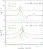 |
Fig. 1 Two examples of infall/outflow signatures of the 12CO line profiles. The optically thin C18O(2–1) emission (scaled for better visibility, shown in green) indicates the systemic velocity. The CO(2–1) and CO(3–2) emission is shown in black and red, respectively. The panels show infall (top ) and outflow (bottom). |
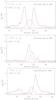 |
Fig. 2 Three examples of infall/outflow signatures of the HCO+(1–0) line profile. Red marks both H13CO+(1–0), which is optically thin, and the systemic velocity of the dense gas. Compared to this the shift of the peak of the HCO+(1–0) emission, in black, becomes clear. The panels show infall (middle and bottom), outflow (bottom right), and a case of central self-absorption, where both peaks are equal (top). The profiles show various degrees of self-absorption. |
3.1.2. The skewness parameter δv
The optically thick HCO+(1–0) line profiles were used for an in-depth study of infall and outflow motions in the clumps. The systemic velocity of a clump was determined from the optically thin H13CO+(1–0) line. Examples of HCO+(1–0) line profiles are shown in Fig. 2. For half of the clumps, the HCO+(1–0) line showed a double-peaked profile with a self-absorption dip. Here, the ratio of the two intensity peaks,  , was used to check whether the source showed blue or red excess in the emission (ratio listed in Table B.2).
When the HCO+(1–0) line profile showed only one peak, we compared its velocity with the velocity of the optically thin H13CO+(1–0) peak. The measure of this shift in velocity is called the skewness parameter. Following the method outlined in Mardones et al. (1997), the skewness parameter δv, is defined as 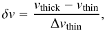 (2)where vthick and vthin are the LSR velocities of the peaks of the optically thick and thin lines, respectively; Δvthin is the line width of the optically thin line. The line width and LSR velocity of the H13CO+(1–0) line were retrieved by Gaussian fits (Table B.3). For the optically thick HCO+(1–0) line, the profiles often showed non-Gaussian shapes; therefore, the position of the peak was determined by eye (also given in Table B.3). After Mardones et al. (1997), we adopt the definition of significant blue and red excess, namely for the former if δv ≤ −0.25 and the latter when δv ≥ 0.25.
The skewness parameter was determined for the HCO+(1–0), HCO+(4–3), and CO(3–2) lines (all listed in Table B.2). For all molecules, the values ranged between –1.5 and 1.5, except for G14.39-00.75B where the δv of the HCO+(1–0) line was –5.79. The latter is due to a very blue shifted HCO+(1–0) peak, most likely caused by a high self-absorption in this source. The clumps in high extinction clouds have skewness parameters similar to values in the literature: –0.5 for UCHii regions (Wyrowski et al. 2006), –1.5 to 1 for HMPOs (Fuller et al. 2005), –1 to 2 for extended green objects (EGOs, Chen et al. 2010), which are shocked regions, and –0.5 for the cluster-forming clump G24.4 (Wu et al. 2005).
Cross correlations of the skewness between the three different molecules (Fig. 3, clumps from peaked and multiply peaked clouds are color coded in light of the evolutionary sequence discussion in Sect. 4.2) show that the HCO+(4–3) line is the least sensitive to infall and/or outflow, while the HCO+(1–0) seems the most sensitive. Most of the HCO+(4–3) lines’ δv values are < |0.25|, while those of the HCO+(1–0) and CO(3–2) lines exhibit a range of skewness. Also, Fuller et al. (2005) found that the transitions with higher critical densities show less infall. These observations suggest that the infall occurs predominantly in the low-density environment, which is in contrast with the increasing infall velocity toward the center that is expected in the collapsing clump model. The observations can possibly be explained by the different optical depths of the HCO+ transitions, because an infall profile requires the transition to be sufficiently opaque. Depending on the density of the infall environment, the transitions with a high critical density might not be opaque enough to observe the skewness profile, while transitions of lower critical density will be already sufficiently optically thick to observe the infall profile. For the HCO+(1–0) and CO(3–2) lines, the skewness seems to be correlated, which makes the infall determination based on these two molecules more reliable.
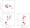 |
Fig. 3 Skewness parameter of the HCO+(1–0) line versus that of the HCO+(4–3) and 12CO(3–2) lines. The dashed lines mark the boundary of significant excess at δv > |0.25|. The blue triangles represent clumps in peaked clouds, while the red squares represent sources in multiply peaked clouds. |
The excess parameter shows the average behavior of the blue excess over the red excess sources. It is defined as E = (Nblue − Nred)/Ntot, where Nred is the number of red excess sources, Nblue the total number of blue excess sources, and Ntot the total number of all sources (Mardones et al. 1997).
Distribution of the skewness parameter per molecule.
Table 3 lists the excess parameter and average skewness parameter by transition. For each transition, we calculated, through the binomial test, the probability P that the distribution between blue and red excess sources occurred by chance. The binomial distribution is defined as  (3)where n is the total number of trials, k the number of successes, and p the success probability. In our case, n is the total number of blue and red excess sources, k the number of blue excess sources, and the success probability p equals 0.5 if the blue and red excess sources are randomly distributed. We can then calculate the possibility that the distribution of the number of blue sources equal or higher than the observed number arises by chance by adding all possibilities P(n, k, p) + P(n, k + 1, p) + ... until k = n.
The small probability P of 7% for HCO+(1–0) line in Table 3 indicates that there are significantly more blue excess sources than expected for a random distribution. On the other hand, the higher CO(3–2) and HCO+(4–3) transitions have a probability of 50%. Hence, the number of blue excess sources is likely by chance and not significant. The results for the CO(2–1) line, P = 0.02, should be treated with care, because the same definitions of blue and red sources do not apply. Due to the possible confusion in the line profiles, the CO(2–1) was just classified based on the peak emission with respect to the C18O(2–1) line without the calculation of δv. Therefore, the numbers in Tables B.2 and 3 have to be taken just as indications. In conclusion, the HCO+(1–0) line shows a significant blue excess and is the best indicator of infall for our sample of clumps. The excess parameter of the HCO+(1–0) line, 0.22, is similar to values found in a previous survey by Fuller et al. (2005) of HMPOs reaching excesses of 0.29 and 0.31. Studies of low-mass star formation also report similar numbers (Mardones et al. 1997; Evans 2003).
3.2. Temperature and density estimations from N2H+(1–0) and (3–2) transitions
The N2H+(1–0) and N2H+(3–2) rotational transitions have hfs arising from the interaction between the molecular electric field gradient and the electric quadrupole moments of the two nitrogen nuclei (Caselli et al. 1995). The N2H+(1–0) rotational transition is split into seven hyperfine components. The three main hyperfine groups were well resolved in our observations (see Fig. 4), and for a few sources we could fit all seven components. In the higher transition, we were barely able to even resolve the three main groups of hfs components (Fig. 4).
For fitting the N2H+(1–0) transition we took the hfs into account by using the hfs method for the line fitting in CLASS2. This method assumes one excitation temperature and one line width for all seven hyperfine components, as well as the fact that the opacity as a function of frequency for each hfs has a gaussian shape. Then, besides the intrinsic line width and integrated intensities, the hfs method also determines the optical depth of the main hfs group. The total optical depth τtot can be calculated from the obtained main hfs group optical depth τmain by multiplying it by the sum of relative intensities of the satellites S as τtot = Sτmain. In case the relative intensities are scaled so that their sum equals unity, the hfs fit directly delivers the total optical depth (the sum of all the hfs optical depths). We calculated the column density of N2H+, NN2H+ (see Eq. (A.3)) following Benson et al. (1998). The results of the N2H+(1–0) line profile fitting; the integrated intensity (including the hyperfine components), total optical depth, and line width are placed together with the excitation temperature and the column density in Table B.4. For N2H+(3–2), Table B.5 lists the parameters obtained by Gaussian fits. We did not observe the hfs as clearly as in the lower transition and could therefore not determine the optical depth for the higher transition.
For sources with τ(1−0), tot ≲ 0.4, which usually also had
high relative errors, we found unrealistically high Tex values
that were much higher than the ammonia rotational temperatures, Trot (Paper I). The CLASS hfs method does not provide good
estimates for excitation temperatures (hence also column densities) when the relative
errors in optical depth are very large ( >40%) and when the optical depth is very small (τ(1−0), tot ≲ 0.4) (see, e.g., Fontani et al. 2006, 2011).
After discarding these sources, the excitation temperatures generally ranged from 3 to
29 K, averaging 8.1 K. In fact, only two sources had a
Tex > 20 K; G017.19+00.81 MM2 (28 K) and MM3 (29 K). We
assumed that the N2H+ gas has a similar kinetic temperature as the NH3 gas and that they are both in local thermal equilibrium (LTE), in which
case the Tex should equal Trot.
However, the determined excitation temperatures were, with the exception of
G017.19+00.81 MM2 and MM3, all lower than the rotational temperature from ammonia. The
difference between the Tex determined here and the Trot determined by ammonia is the N2H+
filling factor. While Tex, is inversely proportional to the
filling factor (see Sect. A.1), the rotational
temperature is an intrinsic temperature (independent of f since it is
solely determined by line ratios). We estimated the filling factor from the ratio of the
excitation temperature of N2H+(1–0) and the NH3
rotational temperature:  (4)The individual filling factors range from 0.2
to 0.8. For clumps G17.19+00.81 MM2, and MM3, we found meaningless filling factors larger
than unity, which is possibly due to an overestimation of the excitation temperature. A
filling factor smaller than unity indicates either that the source size is smaller than
the beam or that the source is clumpy instead of centrally condensed. Alternatively, the N2H+(1–0) line could be sub-thermally excited, a consequence of
densities lower than the critical density. At such densities, a transition’s upper energy
level becomes underpopulated: collisions do not manage to populate it, and the system is
in non-LTE. In this case, the excitation temperature will be lower than the kinetic
temperature, thus mimicking the behavior of a small filling factor.
(4)The individual filling factors range from 0.2
to 0.8. For clumps G17.19+00.81 MM2, and MM3, we found meaningless filling factors larger
than unity, which is possibly due to an overestimation of the excitation temperature. A
filling factor smaller than unity indicates either that the source size is smaller than
the beam or that the source is clumpy instead of centrally condensed. Alternatively, the N2H+(1–0) line could be sub-thermally excited, a consequence of
densities lower than the critical density. At such densities, a transition’s upper energy
level becomes underpopulated: collisions do not manage to populate it, and the system is
in non-LTE. In this case, the excitation temperature will be lower than the kinetic
temperature, thus mimicking the behavior of a small filling factor.
To have another estimate of the filling factor, we performed radiative transfer modeling
to obtain the intrinsic N2H+ column density. In a non-LTE system,
the ratios of line intensities deviate from the LTE predictions and become a function of
density, column density, temperature, and optical depth. In particular, we consider the N2H+(1–0)/N2H+(3–2) line ratio and combine
this with non-LTE radiative transfer modeling using RADEX (van der Tak et al. 2007) and the molecular database LAMBDA (Schöier et al. 2005). Figure 5 shows the integrated intensities of the two N2H+
transitions plotted against each other. We use differently colored symbols for each cloud
class (diffuse, peaked, and multiply peaked) in the graphs shown throughout this paper to
visualize the (possible) behavior for different phases of cloud evolution. The integrated
intensity,  , of the lower transition, N2H+(1–0), exceeded that of N2H+(3–2) by an
average of
, of the lower transition, N2H+(1–0), exceeded that of N2H+(3–2) by an
average of  (5)In this ratio, we assumed that the filling
factor ratio is 1, since it is likely that the filling factors of the two transitions
cancel out as the APEX beam is only slight smaller than the IRAM 30 m beam (Table 2 lists all beamsizes). There are three sources that
lie far from the average: G014.63–00.57 MM1, G017.19+00.81 MM2, and G022.06+00.21 MM1,
which are all bright at 24 μm and contain water masers (see Table B.1).
(5)In this ratio, we assumed that the filling
factor ratio is 1, since it is likely that the filling factors of the two transitions
cancel out as the APEX beam is only slight smaller than the IRAM 30 m beam (Table 2 lists all beamsizes). There are three sources that
lie far from the average: G014.63–00.57 MM1, G017.19+00.81 MM2, and G022.06+00.21 MM1,
which are all bright at 24 μm and contain water masers (see Table B.1).
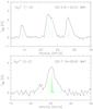 |
Fig. 4 N2H+(1–0) (top) and N2H+(3–2) (bottom) line profiles. The green lines show the locations of the hyperfine components. |
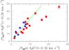 |
Fig. 5 N2H+(1–0) integrated intensity versus N2H+(3–2) integrated intensity for all detected sources. The blue triangles represent clumps in peaked clouds, while the red squares represent sources in multiply peaked clouds. The green solid line marks the trend of the observed ratio of 2.9. |
The observed N2H+ column density is roughly proportional (depending
on the value of Tex, see Eq. (A.3)) with excitation temperature,  for 5 K < Tex < 10 K, which in turn is inversely
proportional with filling factor. Hence, the ratio of observed N2H+
column density (from the N2H+(1–0) line) and the intrinsic column
density calculated by RADEX (based on the N2H+(1–0)/N2H+(3–2) integrated intensity
ratio) can be interpreted as a result of the filling factor of the N2H+(1–0) line. Using RADEX, we estimated the behavior of NN2H+/Δv and nH2 for different values of the N2H+(1–0)/N2H+(3–2) line ratio and the
opacity of N2H+(1–0) for kinetic temperatures of 10, 15, 20, 25 K.
We chose this temperature range based on rotational temperatures derived from the ammonia
observations (see also Table 1). The results are
shown in Fig. 6 and Table 4.
for 5 K < Tex < 10 K, which in turn is inversely
proportional with filling factor. Hence, the ratio of observed N2H+
column density (from the N2H+(1–0) line) and the intrinsic column
density calculated by RADEX (based on the N2H+(1–0)/N2H+(3–2) integrated intensity
ratio) can be interpreted as a result of the filling factor of the N2H+(1–0) line. Using RADEX, we estimated the behavior of NN2H+/Δv and nH2 for different values of the N2H+(1–0)/N2H+(3–2) line ratio and the
opacity of N2H+(1–0) for kinetic temperatures of 10, 15, 20, 25 K.
We chose this temperature range based on rotational temperatures derived from the ammonia
observations (see also Table 1). The results are
shown in Fig. 6 and Table 4.
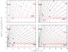 |
Fig. 6 N2H+(1–0) optical depth versus the ratio of N2H+(1–0) and N2H+(3–2) integrated intensities. The four plots represent RADEX calculations with different temperatures: top left 10 K; top right 15 K; bottom left 20 K; bottom right 25 K. The black dashed contours represent the logarithm of the line width times the column density, log (NN2H+/Δv) with a contour step of 0.1. The red dashed contours are log (nH2) with a contour step of 0.2. The lowest and highest contour values are given in each plot. The values of the sources in Table 4 are plotted by black dots. |
Results of RADEX calculations based on the (1–0)/(3–2) N2H+ ratio.
In Fig. 6 we marked the positions of the sources from Table 4 at the intersection of the ratio of the (1–0) and (3–2) N2H+ intensities and the N2H+(1–0) optical depth in the plot calculated with a kinetic temperature closest to the NH3 rotational temperature of the clump. To obtain the intrinsic N2H+ column density, we multiplied NN2H+/Δv by the observed N2H+(1–0) line width. In the plots, we see that a rising Tkin increases the column density for a given optical depth and a line ratio, while the volume density decreases. For the handful of sources that we have measured both N2H+ transitions, we compared the filling factor based on the column density with the one determined from the temperature. On average, the filling factors agreed within 30%. Here we excluded clumps G017.19+00.81 MM2 and MM3, since column density-derived filling factor came out larger than unity, and which confirms that for these sources the derivation of the N2H+ parameters, from which the excitation temperature and column density are calculated, gave unrealistic values.
The RADEX results for the volume density were almost all within a factor two or less of the measured volume density from the 1.2 mm continuum (Table 4). Given the uncertainties in the derivations of both volume densities, we can say that they are in agreement for most of the sources. The N2H+ ratio and the N2H+(1–0) optical depth can therefore be used to estimate the hydrogen volume density and intrinsic N2H+ column density of a clump for a given kinetic temperature.
We estimated the abundance, χ, of N2H+ by
comparing the NN2H+ corrected by the
filling factor from the temperature ratio (for each source individually) to the hydrogen
column density, NH2, measured from the 1.2 mm
continuum (Paper I): 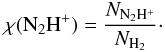 (6)The individual clump abundances are listed in Table B.4, and range from 0.26−4.0 × 10⁻⁹, with a mean of 1.3 × 10⁻⁹. The true abundances
are likely to be slightly lower, since the NH2 is a
beam-averaged column density and contains an unknown filling factor. Taking this into
account, the abundance is in agreement with the value of Pirogov et al. (2007) for high-mass star-forming cores and the results of Ragan et al. (2006); Vasyunina et al. (2011) for IRDCs.
(6)The individual clump abundances are listed in Table B.4, and range from 0.26−4.0 × 10⁻⁹, with a mean of 1.3 × 10⁻⁹. The true abundances
are likely to be slightly lower, since the NH2 is a
beam-averaged column density and contains an unknown filling factor. Taking this into
account, the abundance is in agreement with the value of Pirogov et al. (2007) for high-mass star-forming cores and the results of Ragan et al. (2006); Vasyunina et al. (2011) for IRDCs.
3.3. Presence of young stellar objects
3.3.1. Hot molecular cores: CH3CN and H2CO
CH3CN and H2CO are usually found toward YSOs or hot molecular cores (Mangum & Wootten 1993; Olmi et al. 1996; van der Tak et al. 2000), which are warm (≥100 K) and dense (≥105−106 cm-3) (Kurtz et al. 2000). Both molecules can be used as a tracer of ongoing star formation.
CH3CN is a symmetric-top molecule where each rotational level is split for different projections of angular momentum along the symmetry axis of the molecule labeled by the quantum number K. Within one rotational level, J + 1 → J, the transitions of the K components are determined solely by collisions, and their relative intensities are therefore related to the kinetic temperature of the region (Solomon et al. 1971). The K components with one rotational level are very closely spaced in frequency and can be observed simultaneously with one backend with a bandwidth ≳30 MHz. Under the assumption that the CH3CN(5–4) K = 0, 1, 2, 3, and 4 emission is optically thin and uniformly fills the beam and that all K transitions within this J level are characterized by one temperature, we derived the rotational temperatures, Trot, and the total CH3CN column density following Araya et al. (2005). These authors studied the CH3CN emission toward objects similar to ours (massive star-forming clumps) and showed that it is reasonable to assume the optically thin limit for this line. A beam-filling factor smaller than unity would affect the K levels similarly and hence would have no large influence on the temperature derivation if the filling factor does not vary from one K component to another. The CH3CN column density, however, is affected by the beam-filling factor. Given the beam size of 27′′ against the average angular clump size found at 1.3 mm, ~20′′, the beam-filling factor could be slightly smaller than unity.
We detected the K = 0 to 3 levels, or a subset of these, for several sources; the data were too noisy (1σ rms of 0.9 K) for a K = 4 level detection. All detections, derived Trot, and column densities are given in Table B.6. The CH3CN rotation temperatures were much higher than the NH3 temperatures (see Table B.6 and Fig. 7), since the CH3CN traces warmer gas than ammonia does. For the H2CO(403–304) line, the observed main beam brightness temperatures, LSR velocities, and line widths were determined from Gaussian fits and are listed in Table B.7.
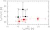 |
Fig. 7 CH3CN rotational temperatures versus NH3 rotational temperatures. Clumps for which the CH3CN temperature had errors smaller than 12 K are red. |
To understand if YSOs are preferably present in denser or more compact clumps, we plotted all the clumps with evidence for an embedded YSO in a size versus the column density graph (Fig. 8). In addition to plotting clumps with evidence of a hot molecular core through the detection of H2CO and CH3CN, we plot clumps with a 24 μm detection (direct evidence of dust heated by an YSO) and SiO emission (evidence of outflows, see Sect. 3.3.2). Apparently, YSOs are found in clumps of all sizes, but, more interestingly, they are mostly found at high column densities. The minimal NH2 at which the H2CO(403–304) line was detected is 4 × 1022 cm-2, while the CH3CN(5–4) K = 0 emission was still observed toward one less dense clump with NH2 = 3 × 1022 cm-2. The column density cut-off is most clearly seen in the 24 μm and SiO line detections; above a column density of 5 × 1022 cm-2, almost all clumps show infrared emission and signs of outflows.
For both the CH3CN and H2CO molecules, there is a general cut-off in the column density at 4 × 1022 cm-2, below which no YSOs are found. This cut-off is slightly lower than the column density of ~1 × 1023 cm-2 theoretically required to form massive stars (0.7 g cm-2, Krumholz & McKee 2008). López-Sepulcre et al. (2010) found a column density threshold of 7.7 × 1022 cm-2, below which the outflow rate decreases rapidly and the outflows are less massive. Hence, while observational data seem to strongly support a column density cutoff for (massive) star formation, they also seem to indicate a slightly lower threshold than theoretically advocated. The difference, however, is not too large, and the observed column densities are beam-averages, which means that if the source size is smaller, we are underestimating the true column density.
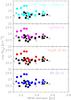 |
Fig. 8 High extinction clumps placed in a diagram of column density versus the FWHM diameter (in pc) derived from the 1.2 mm continuum (Paper I). The detections of MIPS 24 μm emission, H2CO(403–304), CH3CN(5–4) K = 0, and SiO(2–1) are marked in color, black symbols are non-detections. The crosses mark the clumps in diffuse clouds, triangles clumps in peaked clouds, and squares clumps in multiply peaked clouds. |
3.3.2. Outflow: SiO(2–1) emission
Apart from evidently heating their environments, (massive) YSOs drive strong molecular outflows (Beuther et al. 2002), which may remove, in the case of disk accretion, the angular momentum away from the forming star. While mechanisms to accelerate the outflow have been proposed for low-mass star formation (Shu et al. 2000), in the high-mass scenario the acceleration mechanism is not well understood yet.
Interstellar dust grains contain silicates (Draine 2003). Shock waves driven by outflows can sputter Si-bearing compounds in dust grains leading to increased SiO abundances in the post-shock gas (Schilke et al. 1997). Thus, SiO is expected to be associated with ongoing star formation via its formation history. Observations support this, since SiO is more common in more active (or evolved) sources, while very weak in quiescent (hence early) sources (Beuther & Sridharan 2007). Naturally, one also expects to observe wide line widths. We found line widths from ~1.5–7 km s-1 for very weak SiO detections, while for stronger SiO emitting sources the line widths increase up to 26 km s-1. The individual values for all detections are given in Table B.7 along with the main beam brightness temperatures and LSR velocities. The mean noise level of the SiO observations is 0.07 K, which is comparable to previous studies in massive star-forming regions by Beuther & Sridharan (2007) and Motte et al. (2007), which reached noise levels of 0.02 K and 0.10 K, respectively.
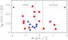 |
Fig. 9 SiO detections against the HCO+(1–0) skewness parameter δv. The green crosses represent sources in diffuse clouds, the blue triangles clumps in peaked clouds, and the red squares sources in multiply peaked clouds. |
We detected the SiO(2–1) transition toward 50% of the whole sample. Of all the SiO-emitting sources, a remarkable majority, 70%, coincided with infall sources (having a HCO+(1–0) skewness parameter, δv ≤ −0.25), as illustrated in Fig. 9. This finding indicates that accretion is accompanied by collimated outflows, which cause the enhancement of SiO. A further 15% of the SiO detections are sources exhibiting expansion (δv ≥ 0.25), and the remaining 15% are sources showing neither expansion nor infall (−0.25 < δv < 0.25). Clumps without SiO detections have HCO+(1–0) skewness parameters divided almost equally between infall (ten clumps) and expansion (eight clumps).
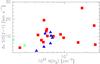 |
Fig. 10 SiO line width against the hydrogen column density NH2. The green crosses represent sources in diffuse clouds, the blue triangles clumps in peaked clouds, and the red squares sources in multiply peaked clouds. |
To check if the SiO line widths, and hence the outflows, are stronger for the more evolved sources, we compared them with the hydrogen column density determined from the 1.2 mm continuum. Figure 10 shows that up to column densities of 1023 cm-2 there is a tendency of increasing line widths with column density. The few clumps that are above this column density limit, G014.63–00.57 MM1, G017.19+00.81 MM2, G022.06+00.21 MM1, and G014.63–00.57 MM2, show no clear trend. The SiO emission was detected toward all multiply peaked clouds, but just toward three peaked clouds (25%) and only two diffuse clouds (18%), singling out the multiply peaked clouds as active regions of star formation.
3.3.3. Prestellar and starless sources
Our sample contained 19 sources with no evidence of a YSO. Of these sources, one-third shows infall in the HCO+(1–0) line profile indicating that these are in a prestellar phase, one-third is expanding according to the HCO+(1–0) skewness parameter, and the last third shows neither infall nor outflow. The sources without any signs of infall or YSOs were defined as starless.
Motte et al. (2007) showed how difficult it is to find high-mass analogies of low-mass starless cores, such as L1521F (Shinnaga et al. 2004), in their study of the Cygnus X complex. Remarkably, they found SiO emission in all of the observed infrared-quiet massive dense cores, indicating that star formation is already ongoing.
In our sample, we found six prestellar and six starless sources. Only half of them contain a clump (an overdensity of typical hydrogen column density of 1022 cm-2, which could be identified by the Miriad routine “sfind”, see Paper I); most of them are too diffuse in the mm continuum. The masses of the prestellar clumps, derived from the 1.2 mm continuum, were greater than their virial masses, indicating that gravity is the dominant force. However, also for the starless clumps, their virial parameters indicate that gravity dominates their internal dynamics. Apparently, it is not merely the lack of gravitational force that separates the starless from the prestellar clumps. The prestellar and starless sources were found in the diffuse and peaked clouds, but not in the multiply peaked clouds, which agrees with the previous indications of the multiply peaked clouds as the most evolved clouds. Most of the starless sources were in diffuse clouds, which are dark in the 24 μm MIPS images. The prestellar sources were generally found in the vicinity of infrared objects, most likely more evolved YSOs. These YSOs are possibly responsible for introducing shocks into their surrounding medium through stellar winds and outflows, thus supporting the formation of higher densities regions where gravitational collapse can occur. This implies that stars form close to other stars, which is a well-known fact and agrees with the observed clustering of newly formed stars (see, for example, Lada & Lada 2003). The limited number of both starless and prestellar sources in a total of 12 clumps, compared to the 31 sources with a YSO indication, agrees with the findings of Motte et al. (2007) that the starless and prestellar phases are short and dynamic.
3.4. CO depletion
As a clump contracts, the level of depletion of C-bearing molecules like CO or CS increases (Kramer et al. 1999; Bergin & Langer 1997). The CO depletion in a clump can therefore be used as a time marker. Observations of massive protostellar objects (Purcell et al. 2009) and clumps in IRDCs (Pillai et al. 2007) show depletion of CO, indicating that these objects are already in a state of collapse and not in the chemically earliest stage. CO depletion as a time marker should be treated with some caution, because heating of the gas (by a YSO) can cause the CO to be desorbed to the gas phase, creating low CO-depletion levels as in the chemically earliest stages around the onset of collapse.
We used C18O, a less common isotopologue of CO, to measure the depletion in the clumps of the high extinction clouds. In contrast to CO, the line profile of C18O lines consisted of one Gaussian without any wings or self-absorption. This is an indication that the C18O(2–1) emission has a low or moderate optical depth, which would agree with previous observations that derived the C18O optical depths by comparing the C18O data with emission from the even rarer C17O (Crapsi et al. 2005; Pillai et al. 2007). Therefore, in this work, we will assume that the C18O(2–1) line is optically thin. The C18O(2–1) line profiles were fitted with a Gaussian. Table B.8 lists our obtained integrated intensities, the LSR velocities, and the line widths.
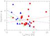 |
Fig. 11 CO depletion versus the rotational temperature derived from NH3. The green crosses represent sources in diffuse clouds, the blue triangles clumps in peaked clouds, and the red squares sources in multiply peaked clouds. The black dashed line marks the trend of an increase in CO depletion with colder temperatures for all the clumps, while the green, blue, and red solid lines mark the trends for the sources in diffuse, peaked, and multiply peaked clouds. |
Infall velocities, mass infall rates, and timescales for the blue excess sources.
The column density of C18O was calculated in the optically thin limit (see Eq. (A.4)) under the assumption of a
beam filling factor of unity, which is likely for a beam of 11′′ and clumps that have an
average size of 20′′ in the 1.2 mm continuum. Second, we assume LTE and equate the
excitation temperature to the rotational temperature, Trot,
derived from the NH3(1, 1) and NH3(2, 2) transitions. In very dense
and cold regions, where NH3 inversion transitions are dominated by collisions
rather than by radiative excitations and de-excitations, Trot
is a good measure for the kinetic temperature of the system (Walmsley & Ungerechts 1983; Danby et al. 1988). The background temperature was taken at 2.73 K. With the total
column density of C18O, NC18O, known, we
calculated the abundance of C18O relative to H2, χC18O, by comparing it to the hydrogen column
density:  (7)The canonical number for χC18O in the nearby ISM is 1.7 × 10⁻⁷ (Frerking et al. 1982). At
larger distances towards the molecular ring and the Galactic center, this value is
expected to be higher (Wilson & Rood 1994),
which would increase the CO depletion we measured. The ratio between the observed
abundance, χobs, and the canonical value for the abundance, χcanonical, then resulted in η the CO
depletion factor:
(7)The canonical number for χC18O in the nearby ISM is 1.7 × 10⁻⁷ (Frerking et al. 1982). At
larger distances towards the molecular ring and the Galactic center, this value is
expected to be higher (Wilson & Rood 1994),
which would increase the CO depletion we measured. The ratio between the observed
abundance, χobs, and the canonical value for the abundance, χcanonical, then resulted in η the CO
depletion factor:  (8)All derived quantities, NC18O, NH2,
χC18O, and η are listed in Table B.9. In most of the clumps,
C18O appears to be depleted. We find a CO depletion of
η = 0.5–5.5 with an average of 2.3, which is slightly lower than what is
found in clumps of IRDCs (η = 2–10, Pillai et al. 2007). Observations by, e.g., Kramer et al. (1999) and Bacmann et al. (2003) have shown that molecular depletion is enhanced at lower temperatures. In Fig. 11, we plot for all clumps the CO depletion
against the rotational temperature. While Kramer et al. (1999) found an strong exponential dependence of CO depletion with temperature,
our data are too scattered to differentiate between linear and exponential behavior.
Nevertheless we can see that higher η corresponds on average to colder
sources (dashed black line).
(8)All derived quantities, NC18O, NH2,
χC18O, and η are listed in Table B.9. In most of the clumps,
C18O appears to be depleted. We find a CO depletion of
η = 0.5–5.5 with an average of 2.3, which is slightly lower than what is
found in clumps of IRDCs (η = 2–10, Pillai et al. 2007). Observations by, e.g., Kramer et al. (1999) and Bacmann et al. (2003) have shown that molecular depletion is enhanced at lower temperatures. In Fig. 11, we plot for all clumps the CO depletion
against the rotational temperature. While Kramer et al. (1999) found an strong exponential dependence of CO depletion with temperature,
our data are too scattered to differentiate between linear and exponential behavior.
Nevertheless we can see that higher η corresponds on average to colder
sources (dashed black line).
Figure 11 shows that clumps in diffuse clouds (green crosses and green line) and peaked clouds (blue triangles and blue line) indeed follow the trend of higher CO depletion with colder temperatures. For clumps in multiply peaked clouds (red squares and red line), the situation is different; the clumps have a large spread in temperature as well as η, and on average the opposite trend is seen: increasing η with higher temperature. This is mainly caused by a few clumps with high temperature and high η, G017.19+0.81 MM2, G014.63–00.63 MM1, and G022.06+0.21 MM1, all three of which have dust column densities above 1023 cm-2 and water masers. Possibly these sources were heated so fast by the embedded YSO that the CO was not freed into the gas phase yet and the depletion values are thus still high.
4. Discussion
4.1. Infall velocities
In Sect. 3.1, we determined by binomial tests that
the HCO+(1–0) line was the best suited of the molecular transitions that we had
observed to study infall. For sources that had a double-peaked HCO+(1–0) line
profile, indicating a systemic infalling motion, we calculated the infall velocity vin according to Myers et al. (1996) as 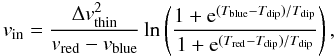 (9)where vred and vblue are the LSR velocities of the red and blue peaks,
whose main beam temperatures are given by Tred and Tblue, respectively, and Tdip is the main beam temperature of the dip between the
two peaks. All these quantities refer to the spectral shape of the optically thick line,
except for Δvthin. With the volume density of the clump nH2 and clump radius R, the
infall velocity can be converted to a mass infall rate Ṁin
(after Myers et al. 1996):
(9)where vred and vblue are the LSR velocities of the red and blue peaks,
whose main beam temperatures are given by Tred and Tblue, respectively, and Tdip is the main beam temperature of the dip between the
two peaks. All these quantities refer to the spectral shape of the optically thick line,
except for Δvthin. With the volume density of the clump nH2 and clump radius R, the
infall velocity can be converted to a mass infall rate Ṁin
(after Myers et al. 1996):  (10)where μ = 2.33 the mean
molecular weight and mH the mass of an hydrogen atom. For the
clump nH2 and clump radius R, we
took the volume density and clump radius determined in Paper I from 1.2 mm dust continuum
observations.
(10)where μ = 2.33 the mean
molecular weight and mH the mass of an hydrogen atom. For the
clump nH2 and clump radius R, we
took the volume density and clump radius determined in Paper I from 1.2 mm dust continuum
observations.
For low-mass star formation, the mass infall rates onto a protostar are between a few times ~10-5 M⊙ yr-1 (Palla & Stahler 1993; Kirk et al. 2005) and ~10-6 M⊙ yr-1 (Whitney et al. 1997). This is too low to form high-mass stars, since their prestellar phase is much shorter, less than 3 × 10⁴ yr, according to Motte et al. (2007), which would mean a mass infall rate of 3 × 10⁻⁴ M⊙ yr-1 to form a 10 M⊙ star. Theoretical models predict a mass accretion onto a high-mass protostellar core (at radii <0.1 pc) of Ṁin of 10-3 M⊙ yr-1 (McKee & Tan 2003; Banerjee & Pudritz 2007). Observations of massive clumps (with typical radii >0.1 pc) find mass infall rates of 10-3−10-4 M⊙ yr-1 (Fuller et al. 2005; Peretto et al. 2006). In high-resolution observations of high-mass protostellar cores, the mass infall rate is indeed higher and covers the predicted order of magnitude (10-2−10-4 M⊙ yr-1, Beltrán et al. 2006, 2008). Our mass infall results, given in Table 5, fall in the range of the observed values for massive star-forming clumps.
To explore further the mass infall rate, we calculated the infall timescale using the
clump mass obtained from the 1.2 mm continuum (Paper I):  yr. This timescale can be compared with
the free-fall timescale τff = 3.3 × 10⁷ n−1/2 yr, which was
calculated using the density obtained from the same 1.2 mm continuum observations
(Paper I). Both timescales are given in Table 5. In
general, the free-fall timescale is longer than the estimated infall timescale, which
indicates that the mass infall rate calculated in Eq. (10) is likely overestimated. The formula in Eq. (10) assumes a spherically symmetric infall of
the entire clump, while most likely the HCO+(1–0) emission is originating in an
optically thick low-density layer in the outer parts of the clump (see also López-Sepulcre et al. 2010). We also calculated the HCO+(4–3) infall velocities and mass infall rates for the few sources that
showed a double-peaked blue-excess line profile (Table 5). Unfortunately, the error in the infall velocity of G024.94–00.15 MM1 was
quite high, leaving only G014.63–00.57 MM1 to serve as a comparison. For the latter, the
infall velocity derived from the higher excitation HCO+(4–3) line profile is
half of the one derived from the HCO+(1–0) line profile, and the HCO+(4–3) infall timescale is twice the HCO+(1–0) timescale. At
least for this one source, we find an indication that the HCO+(1–0) infall
velocities and mass infall rates are indeed overestimated.
yr. This timescale can be compared with
the free-fall timescale τff = 3.3 × 10⁷ n−1/2 yr, which was
calculated using the density obtained from the same 1.2 mm continuum observations
(Paper I). Both timescales are given in Table 5. In
general, the free-fall timescale is longer than the estimated infall timescale, which
indicates that the mass infall rate calculated in Eq. (10) is likely overestimated. The formula in Eq. (10) assumes a spherically symmetric infall of
the entire clump, while most likely the HCO+(1–0) emission is originating in an
optically thick low-density layer in the outer parts of the clump (see also López-Sepulcre et al. 2010). We also calculated the HCO+(4–3) infall velocities and mass infall rates for the few sources that
showed a double-peaked blue-excess line profile (Table 5). Unfortunately, the error in the infall velocity of G024.94–00.15 MM1 was
quite high, leaving only G014.63–00.57 MM1 to serve as a comparison. For the latter, the
infall velocity derived from the higher excitation HCO+(4–3) line profile is
half of the one derived from the HCO+(1–0) line profile, and the HCO+(4–3) infall timescale is twice the HCO+(1–0) timescale. At
least for this one source, we find an indication that the HCO+(1–0) infall
velocities and mass infall rates are indeed overestimated.
4.2. Evolutionary sequence
In Paper I, we defined three classes of high extinction clouds, based on the contrast of the clump to the cloud in the 1.2 mm continuum and the number of clumps per cloud. These clouds comprise diffuse clouds, clouds with a low clump-to-cloud column density contrast CNH2 < 2, peaked clouds, clouds with higher contrast 2 < CNH2 < 3 having at least one clump, multiply peaked clouds, clouds with still higher contrast CNH2 > 3 that generally contained several clumps. Here, we review all the results in light of the hypothetical evolutionary sequence we proposed, i.e., from the quiescent diffuse clouds to the peaked ones, and finally to the multiply peaked clouds.
4.2.1. Diffuse clouds
For the class of diffuse clouds, more than half of the investigated sources were not well-defined clumps but positions of diffuse emission within a cloud. The skewness parameter analysis found a slight excess of blue sources, indicating infall, but the binomial test showed that this result is not significant (see Table 6). The diffuse clouds are likely the phase where the clumps are beginning to collapse. This would agree with the clump masses found in Paper I, where on average we found less massive clumps in the diffuse clouds than in the peaked or multiply peaked clouds (see also Table 1). Moreover, few YSO/hot core indications were found toward clumps in diffuse clouds, and half of the starless and prestellar sources were found toward the diffuse clouds (the other half was found toward the peaked clouds). A young evolutionary stage can also be identified by the CO depletion, since CO depletion requires a certain density (>few 104 cm-3, Kramer et al. 1999; Bergin & Tafalla 2007). Low depletion levels can indicate that the clump has not yet reached a high enough density. The mean depletion level of clumps in diffuse clouds (η = 1.9) was slightly lower than that found toward the clumps in peaked and multiply peaked clouds (η = 2.3). The depletion timescale, τd ~ 5 × 10⁹/nH2 (Bergin & Tafalla 2007), is ~4 × 10⁴ yr for clumps in diffuse clouds, which is slightly longer than that for in peaked clouds (~3 × 10⁴ yr) and multiply peaked clouds (~2 × 10⁴ yr).
Infall properties from the HCO+(1–0) line profile for different classes of clouds.
4.2.2. Peaked clouds
In the peaked clouds, the distribution of blue and red sources from the HCO+(1–0) line profile significantly favors the blue sources with infall. The excess parameter was 0.53 with only a 1% possibility for this distribution to arise by chance (Table 6). Apparently, most clumps in the peaked clouds are accreting material. The infall velocities and mass accretion rates for peaked (as well as the one for multiply peaked) clouds have a very wide range, whose mean lies far above the infall velocity/mass accretion rate of the diffuse clouds. All the SiO detections of clumps in peaked clouds coincide with sources that show infall based on the HCO+(1–0) skewness parameter (Fig. 9). The strong correlation between the infall characteristics and SiO outflows shows that accretion is accompanied by collimated outflows, which leads to an enhancement of SiO. This correlation does not exist for the earlier or later classes.
4.2.3. Multiply peaked clouds
Among the multiply peaked clouds, there were almost equal numbers of blue and red excess sources (based on the HCO+(1–0) skewness). These clouds seem to be hosting clumps in a variety of evolutionary stages: from clumps with still ongoing accretion to clumps where the feedback from the formed young stars halts further accretion.
Many clumps in these clouds presented SiO emission. Figure 9 shows that the number of clumps with SiO emission showing infall is about equal to those showing expansion (both infall and expansion characteristics are based on the HCO+(1–0) skewness parameter), meaning that the outflow continues even after large-scale infall has finished.
The volume density of the multiply peaked clouds, nH2 > 105 cm-3, is much larger than what is found for the peaked clouds. Multiply peaked clouds have the highest detection rate of the CH3CN(5–4) K = 0 and H2CO(403–304) lines, indicating that this class contains the most YSOs or hot molecular cores. In Paper I, we already found that the NH3 rotational temperatures were on average higher for clumps in multiply peaked clouds than for the other classes (Table 1). The K levels of the CH3CN(5–4) line allowed a handful of rotational temperature estimates, ranging between 23 and 34 K. The increasing evidence for YSOs is likely the reason for the broadening of the line width found toward clumps in this class (observed for the N2H+(1–0), NH3(1, 1), C18O(2–1), and H13CO+(1–0) lines) by increasing turbulence.
Finally, three clumps in the multiply peaked clouds, G014.63-00.57 MM1, G017.19+00.81 MM2, and G022.06 +00.21 MM1, all show various characteristics that are different to the properties of the bulk of the sample. Examples include their SiO intensity against column density, the CO depletion against temperature, and their N2H+(1–0)/N2H+(3–2) ratio. While these clumps have strong outflows, suggested by their SiO emission and the presence of water masers, they also have very high column densities (theoretically enough to form massive stars, e.g., Krumholz & McKee 2008). They show strong CO depletion values while having elevated temperatures ( ~20 K) due to the rapid heating of the environment by the YSO. Most likely, these three clumps are actively forming massive YSOs, which is why they have such extreme properties.
5. Summary
We performed spectral line observations of several molecules using the IRAM 30 m and the APEX telescopes toward a sample of clumps in high extinction clouds spanning various evolutionary stages. The skewness parameter was used to classify sources based on their line profiles as infall sources or outflow/expanding sources. The HCO+(1–0) and CO(3–2) lines were found to be more sensitive to infall and outflow than the HCO+(4–3) line. Only the HCO+(1–0) profiles showed a significant excess of infall sources, and therefore the HCO+(1–0) line profile was found to be most effective to investigate infall profiles.
SiO emission, which is thought to be a tracer of shocks, was predominantly detected toward sources with infall. This finding is consistent with a scenario in which accretion is accompanied by collimated outflows that lead to an enhancement of SiO.
Between the three cloud classes, the peaked clouds have a significant high excess of infall sources, while for the other classes no significant excess was found. Possibly, the infall phase has not yet begun in most diffuse clouds and already has come to an end in some of the clumps of the multiply peaked clouds. The infall velocities and mass infall rates suggest an increasing trend when going from the diffuse clouds (1.5 × 10⁻³ M⊙ yr-1) to the peaked (and multiply peaked) clouds (1.5–16 × 10-3 M⊙ yr-1) suggesting that mass infall increases in these later stages. More measurements of clumps in diffuse clouds are, however, necessary to confirm this.
From RADEX calculations, we found that the ratio of the N2H+(1–0) to N2H+(3–2) integrated intensity is sensitive to the hydrogen volume density, and together with the N2H+(1–0) optical depth can be used to derive good estimates of not only the hydrogen volume density but also the intrinsic N2H+ column density. Apart from the ammonia rotational temperatures, determined in Paper I, we added several other temperature estimates. All estimates converge to a temperature range between 10 and 40 K, where the higher value is determined by CH3CN, a molecule usually found in hot cores and UCHii regions. Similarly, various density estimates place the density in the order of 105 cm-3.
The presence of YSOs in the clumps of the high extinction clouds was established by 24 μm emission, but also indirect evidence through outflows (SiO emission) and the presence of hot molecular cores through CH3CN and H2CO emission was gathered. We find that most of the YSOs are located in clumps of peaked and multiply peaked clouds, while almost no YSO indications were present in diffuse clouds. The presence of an YSO seems independent of the physical size of the clump, since YSOs are found over a large range of clump diameters. However, there seems to be (hydrogen) column density cutoff at (4−5) × 1022 cm-2, below which few or no YSOs are found. The cutoff is most clear in the 24 μm emission and in the presence of SiO emission.
In summary, the diffuse clouds seem to contain clumps that are on the verge of infall. The first stages of star formation are ongoing in the peaked clouds, since a majority of the clumps is infalling and many clumps also show outflows. The multiply peaked clouds harbor the more evolved clumps, where infall has already stopped in some of them, and generally we find indications of YSOs. Hence, the cloud morphology seems to have a direct connection with the evolutionary stage of the objects forming inside.
Online material
Molecular line survey overview.
Infall and outflow study using the HCO+(1–0), CO(2–1), HCO+(4–3) and CO(3–2) lines.
Molecular line survey results for HCO+(1–0) and H13CO+(1–0).
Properties of N2H+(1–0) based on Gaussian fits.
Observed properties of N2H+(3–2) and HCO+(4–3).
Star formation tracers (ii): K levels of CH3CN(5–4).
Star formation tracers (i): SiO(2–1) and H2CO(403–304) based on Gaussian fits.
Observed properties of C18O(2–1) based on Gaussian fits.
Derived abundance and depletion from the C18O(2–1) line.
The off position is an observation of “blank” sky, which is observed to remove the instrumental bandpass structure.
Acknowledgments
We would like to express our thanks to Floris van der Tak and Malcolm Walmsley for their constructive comments that lead to a much improved manuscript. We are grateful for the help and assistance of the staff of both the IRAM 30 m and the APEX 12m telescopes during the observations. KLJR is funded by an ASI fellowship under contract number I/005/11/0.
References
- Araya, E., Hofner, P., Kurtz, S., Bronfman, L., & DeDeo, S. 2005, ApJS, 157, 279 [NASA ADS] [CrossRef] [Google Scholar]
- Bacmann, A., Lefloch, B., Ceccarelli, C., et al. 2003, ApJ, 585, L55 [NASA ADS] [CrossRef] [EDP Sciences] [Google Scholar]
- Banerjee, R., & Pudritz, R. E. 2007, ApJ, 660, 479 [NASA ADS] [CrossRef] [Google Scholar]
- Beltrán, M. T., Cesaroni, R., Codella, C., et al. 2006, Nature, 443, 427 [NASA ADS] [CrossRef] [PubMed] [Google Scholar]
- Beltrán, M. T., Cesaroni, R., Moscadelli, L., et al. 2008, in Massive Star Formation: Observations Confront Theory, eds. H. Beuther, H. Linz, & T. Henning, ASP Conf. Ser., 387, 71 [Google Scholar]
- Benson, P. J., Caselli, P., & Myers, P. C. 1998, ApJ, 506, 743 [NASA ADS] [CrossRef] [Google Scholar]
- Bergin, E. A., & Langer, W. D. 1997, ApJ, 486, 316 [NASA ADS] [CrossRef] [Google Scholar]
- Bergin, E. A., & Tafalla, M. 2007, ARA&A, 45, 339 [NASA ADS] [CrossRef] [Google Scholar]
- Beuther, H., & Sridharan, T. K. 2007, ApJ, 668, 348 [NASA ADS] [CrossRef] [Google Scholar]
- Beuther, H., Schilke, P., Sridharan, T. K., et al. 2002, A&A, 383, 892 [NASA ADS] [CrossRef] [EDP Sciences] [Google Scholar]
- Caselli, P., Myers, P. C., & Thaddeus, P. 1995, ApJ, 455, L77 [NASA ADS] [CrossRef] [Google Scholar]
- Chen, X., Shen, Z.-Q., Li, J.-J., Xu, Y., & He, J.-H. 2010, ApJ, 710, 150 [NASA ADS] [CrossRef] [Google Scholar]
- Churchwell, E., Walmsley, C. M., & Wood, D. O. S. 1992, A&A, 253, 541 [NASA ADS] [Google Scholar]
- Crapsi, A., Caselli, P., Walmsley, C. M., et al. 2005, ApJ, 619, 379 [Google Scholar]
- Danby, G., Flower, D. R., Valiron, P., Schilke, P., & Walmsley, C. M. 1988, MNRAS, 235, 229 [NASA ADS] [CrossRef] [Google Scholar]
- Draine, B. T. 2003, ARA&A, 41, 241 [NASA ADS] [CrossRef] [Google Scholar]
- Evans,II, N. J. 1999, ARA&A, 37, 311 [NASA ADS] [CrossRef] [Google Scholar]
- Evans, II, N. 2003, in SFChem 2002: Chemistry as a Diagnostic of Star Formation, eds. C. L. Curry, & M. Fich, 157 [Google Scholar]
- Fazio, G. G., Hora, J. L., Allen, L. E., et al. 2004, ApJS, 154, 10 [NASA ADS] [CrossRef] [Google Scholar]
- Fontani, F., Caselli, P., Crapsi, A., et al. 2006, A&A, 460, 709 [NASA ADS] [CrossRef] [EDP Sciences] [Google Scholar]
- Fontani, F., Palau, A., Caselli, P., et al. 2011, A&A, 529, L7 [NASA ADS] [CrossRef] [EDP Sciences] [Google Scholar]
- Frerking, M. A., Langer, W. D., & Wilson, R. W. 1982, ApJ, 262, 590 [NASA ADS] [CrossRef] [Google Scholar]
- Fuller, G. A., Williams, S. J., & Sridharan, T. K. 2005, A&A, 442, 949 [NASA ADS] [CrossRef] [EDP Sciences] [Google Scholar]
- Indebetouw, R., Mathis, J. S., Babler, B. L., et al. 2005, ApJ, 619, 931 [NASA ADS] [CrossRef] [Google Scholar]
- Kirk, J. M., Ward-Thompson, D., & André, P. 2005, MNRAS, 360, 1506 [NASA ADS] [CrossRef] [Google Scholar]
- Klein, B., Philipp, S. D., Krämer, I., et al. 2006, A&A, 454, L29 [NASA ADS] [CrossRef] [EDP Sciences] [Google Scholar]
- Kramer, C., Alves, J., Lada, C. J., et al. 1999, A&A, 342, 257 [NASA ADS] [Google Scholar]
- Krumholz, M. R., & McKee, C. F. 2008, Nature, 451, 1082 [NASA ADS] [CrossRef] [PubMed] [Google Scholar]
- Kurtz, S., Cesaroni, R., Churchwell, E., Hofner, P., & Walmsley, C. M. 2000, Protostars and Planets IV, 299 [Google Scholar]
- Kutner, M. L., & Ulich, B. L. 1981, ApJ, 250, 341 [NASA ADS] [CrossRef] [Google Scholar]
- Lada, C. J., & Lada, E. A. 2003, ARA&A, 41, 57 [NASA ADS] [CrossRef] [Google Scholar]
- Leung, C. M., & Brown, R. L. 1977, ApJ, 214, L73 [NASA ADS] [CrossRef] [Google Scholar]
- López-Sepulcre, A., Cesaroni, R., & Walmsley, C. M. 2010, A&A, 517, A66 [NASA ADS] [CrossRef] [EDP Sciences] [Google Scholar]
- Mangum, J. G., & Wootten, A. 1993, ApJS, 89, 123 [NASA ADS] [CrossRef] [Google Scholar]
- Mardones, D., Myers, P. C., Tafalla, M., et al. 1997, ApJ, 489, 719 [NASA ADS] [CrossRef] [Google Scholar]
- McKee, C. F., & Tan, J. C. 2003, ApJ, 585, 850 [NASA ADS] [CrossRef] [MathSciNet] [Google Scholar]
- Motte, F., Bontemps, S., Schilke, P., et al. 2007, A&A, 476, 1243 [NASA ADS] [CrossRef] [EDP Sciences] [Google Scholar]
- Myers, P. C., Mardones, D., Tafalla, M., Williams, J. P., & Wilner, D. J. 1996, ApJ, 465, L133 [NASA ADS] [CrossRef] [Google Scholar]
- Olmi, L., Cesaroni, R., Neri, R., & Walmsley, C. M. 1996, A&A, 315, 565 [NASA ADS] [Google Scholar]
- Palla, F., & Stahler, S. W. 1993, ApJ, 418, 414 [NASA ADS] [CrossRef] [Google Scholar]
- Peretto, N., André, P., & Belloche, A. 2006, A&A, 445, 979 [NASA ADS] [CrossRef] [EDP Sciences] [Google Scholar]
- Pety, J. 2005, in SF2A-2005: Semaine de l’Astrophysique Française, eds. F. Casoli, T. Contini, J. M. Hameury, & L. Pagani, 721 [Google Scholar]
- Pillai, T., Wyrowski, F., Hatchell, J., Gibb, A. G., & Thompson, M. A. 2007, A&A, 467, 207 [NASA ADS] [CrossRef] [EDP Sciences] [Google Scholar]
- Pirogov, L., Zinchenko, I., Caselli, P., & Johansson, L. E. B. 2007, A&A, 461, 523 [NASA ADS] [CrossRef] [EDP Sciences] [Google Scholar]
- Purcell, C. R., Balasubramanyam, R., Burton, M. G., et al. 2006, MNRAS, 367, 553 [NASA ADS] [CrossRef] [Google Scholar]
- Purcell, C. R., Minier, V., Longmore, S. N., et al. 2009, A&A, 504, 139 [NASA ADS] [CrossRef] [EDP Sciences] [Google Scholar]
- Ragan, S. E., Bergin, E. A., Plume, R., et al. 2006, ApJS, 166, 567 [NASA ADS] [CrossRef] [Google Scholar]
- Risacher, C., Vassilev, V., Monje, R., et al. 2006, A&A, 454, L17 [NASA ADS] [CrossRef] [EDP Sciences] [Google Scholar]
- Rygl, K. L. J., Wyrowski, F., Schuller, F., & Menten, K. M. 2010, A&A, 515, A42 (Paper I) [Google Scholar]
- Schilke, P., Walmsley, C. M., Pineaudes Forets, G., & Flower, D. R. 1997, A&A, 321, 293 [NASA ADS] [Google Scholar]
- Schöier, F. L., van der Tak, F. F. S., van Dishoeck, E. F., & Black, J. H. 2005, A&A, 432, 369 [NASA ADS] [CrossRef] [EDP Sciences] [Google Scholar]
- Shinnaga, H., Ohashi, N., Lee, S., & Moriarty-Schieven, G. H. 2004, ApJ, 601, 962 [NASA ADS] [CrossRef] [Google Scholar]
- Shu, F. H., Najita, J. R., Shang, H., & Li, Z. 2000, Protostars and Planets IV, 789 [Google Scholar]
- Solomon, P. M., Jefferts, K. B., Penzias, A. A., & Wilson, R. W. 1971, ApJ, 168, L107 [NASA ADS] [CrossRef] [Google Scholar]
- Tafalla, M., Myers, P. C., Caselli, P., Walmsley, C. M., & Comito, C. 2002, ApJ, 569, 815 [NASA ADS] [CrossRef] [Google Scholar]
- van der Tak, F. F. S., van Dishoeck, E. F., & Caselli, P. 2000, A&A, 361, 327 [NASA ADS] [Google Scholar]
- van der Tak, F. F. S., Black, J. H., Schöier, F. L., Jansen, D. J., & van Dishoeck, E. F. 2007, A&A, 468, 627 [NASA ADS] [CrossRef] [EDP Sciences] [Google Scholar]
- Vasyunina, T., Linz, H., Henning, T., et al. 2011, A&A, 527, A88 [NASA ADS] [CrossRef] [EDP Sciences] [Google Scholar]
- Walmsley, C. M., & Ungerechts, H. 1983, A&A, 122, 164 [NASA ADS] [Google Scholar]
- Whitney, B. A., Kenyon, S. J., & Gomez, M. 1997, ApJ, 485, 703 [NASA ADS] [CrossRef] [Google Scholar]
- Wilson, T. L., & Rood, R. 1994, ARA&A, 32, 191 [NASA ADS] [CrossRef] [Google Scholar]
- Wu, Y., Zhu, M., Wei, Y., et al. 2005, ApJ, 628, L57 [NASA ADS] [CrossRef] [Google Scholar]
- Wyrowski, F., Heyminck, S., Güsten, R., & Menten, K. M. 2006, A&A, 454, L95 [NASA ADS] [CrossRef] [EDP Sciences] [Google Scholar]
- Zhou, S., Evans, II, N. J., Koempe, C., & Walmsley, C. M. 1993, ApJ, 404, 232 [NASA ADS] [CrossRef] [Google Scholar]
Appendix A: Formulas and equations used
A.1. N2H+
The excitation temperature Tex can be calculated as ![Mathematical equation: \appendix \setcounter{section}{1} \begin{equation} T_\mathrm{ex}=\frac{h\nu/k}{\ln \left[\frac{h\nu/k}{A/(\tau_\mathrm{m} f)} +1\right]}, \end{equation}](/articles/aa/full_html/2013/01/aa19574-12/aa19574-12-eq218.png) (A.1)where A = τmf(Jν(T) + Jν(Tbg) is the outcome of the CLASS hfs method fitting. Using ln (ϵ + 1) ≃ ϵ, one can simplify the above equation as
(A.1)where A = τmf(Jν(T) + Jν(Tbg) is the outcome of the CLASS hfs method fitting. Using ln (ϵ + 1) ≃ ϵ, one can simplify the above equation as  (A.2)If we ignore the “+1” in the above equation, we find that Tex ∝ 1/f. Since the average Tex was found to be around 10 K, ignoring the “+1” in the above equation would lead to an uncertainty of (on average) 10%.
We calculated the column density of N2H+, NN2H+, following Benson et al. (1998): ![Mathematical equation: \appendix \setcounter{section}{1} \begin{equation} N_{\mathrm{N_2H^+}} = 3.3\times10^{11}\frac{\tau_\mathrm{tot} \Delta v T_\mathrm{ex}}{1-{\rm e}^{-4.47/T_\mathrm{ex}}}~\mathrm{\left[cm^{-2}\right]}, \label{eq:n2hp} \end{equation}](/articles/aa/full_html/2013/01/aa19574-12/aa19574-12-eq223.png) (A.3)where Δv is the line width obtained from the hyperfine fit and Tex is the excitation temperature.
(A.3)where Δv is the line width obtained from the hyperfine fit and Tex is the excitation temperature.
A.2. CO
In LTE, the total column density, Ntot, of the CO molecule can be calculated from the integrated main beam brightness temperature of an optically thin line as follows:  (A.4)
(A.4)
| where | h | Planck constant |
| k | the Boltzmann constant | |
| S | line strength | |
| μ D | the dipole moment of the molecule | |
| T ex | the excitation temperature | |
| Q(Tex) | partition function at Tex, | |
| Q(Tex) ≃ 0.38(Tex + 0.88) | ||
| g u | the rotational degeneracy for the upper energy | |
| g K | the K degeneracy | |
| g nuc | the nuclear degeneracy | |
| E u | the energy of the upper level | |
| ν | the transition frequency | |
| Jν(T) |  |
The properties of the C18O J = 2 → 1 transition are: S = Ju/(2Ju + 1) = 0.4, where Ju is the angular momentum quantum number of the upper J level, μD = 0.1098 Debye = 0.1098 × 10⁻¹⁸ e.s.u., gu = 2Ju + 1 = 5, gK = 1, gnuc = 1, Eu = k × 15.81 erg, and ν = 219.56 GHz.
The general formula for the CO column density, valid in the optically thick and thin regime is  (A.5)where all the quantities are as defined above.
All Tables
Infall velocities, mass infall rates, and timescales for the blue excess sources.
Infall properties from the HCO+(1–0) line profile for different classes of clouds.
Infall and outflow study using the HCO+(1–0), CO(2–1), HCO+(4–3) and CO(3–2) lines.
All Figures
|
Fig. 1 Two examples of infall/outflow signatures of the 12CO line profiles. The optically thin C18O(2–1) emission (scaled for better visibility, shown in green) indicates the systemic velocity. The CO(2–1) and CO(3–2) emission is shown in black and red, respectively. The panels show infall (top ) and outflow (bottom). |
| In the text | |
|
Fig. 2 Three examples of infall/outflow signatures of the HCO+(1–0) line profile. Red marks both H13CO+(1–0), which is optically thin, and the systemic velocity of the dense gas. Compared to this the shift of the peak of the HCO+(1–0) emission, in black, becomes clear. The panels show infall (middle and bottom), outflow (bottom right), and a case of central self-absorption, where both peaks are equal (top). The profiles show various degrees of self-absorption. |
| In the text | |
|
Fig. 3 Skewness parameter of the HCO+(1–0) line versus that of the HCO+(4–3) and 12CO(3–2) lines. The dashed lines mark the boundary of significant excess at δv > |0.25|. The blue triangles represent clumps in peaked clouds, while the red squares represent sources in multiply peaked clouds. |
| In the text | |
|
Fig. 4 N2H+(1–0) (top) and N2H+(3–2) (bottom) line profiles. The green lines show the locations of the hyperfine components. |
| In the text | |
|
Fig. 5 N2H+(1–0) integrated intensity versus N2H+(3–2) integrated intensity for all detected sources. The blue triangles represent clumps in peaked clouds, while the red squares represent sources in multiply peaked clouds. The green solid line marks the trend of the observed ratio of 2.9. |
| In the text | |
|
Fig. 6 N2H+(1–0) optical depth versus the ratio of N2H+(1–0) and N2H+(3–2) integrated intensities. The four plots represent RADEX calculations with different temperatures: top left 10 K; top right 15 K; bottom left 20 K; bottom right 25 K. The black dashed contours represent the logarithm of the line width times the column density, log (NN2H+/Δv) with a contour step of 0.1. The red dashed contours are log (nH2) with a contour step of 0.2. The lowest and highest contour values are given in each plot. The values of the sources in Table 4 are plotted by black dots. |
| In the text | |
|
Fig. 7 CH3CN rotational temperatures versus NH3 rotational temperatures. Clumps for which the CH3CN temperature had errors smaller than 12 K are red. |
| In the text | |
|
Fig. 8 High extinction clumps placed in a diagram of column density versus the FWHM diameter (in pc) derived from the 1.2 mm continuum (Paper I). The detections of MIPS 24 μm emission, H2CO(403–304), CH3CN(5–4) K = 0, and SiO(2–1) are marked in color, black symbols are non-detections. The crosses mark the clumps in diffuse clouds, triangles clumps in peaked clouds, and squares clumps in multiply peaked clouds. |
| In the text | |
|
Fig. 9 SiO detections against the HCO+(1–0) skewness parameter δv. The green crosses represent sources in diffuse clouds, the blue triangles clumps in peaked clouds, and the red squares sources in multiply peaked clouds. |
| In the text | |
|
Fig. 10 SiO line width against the hydrogen column density NH2. The green crosses represent sources in diffuse clouds, the blue triangles clumps in peaked clouds, and the red squares sources in multiply peaked clouds. |
| In the text | |
|
Fig. 11 CO depletion versus the rotational temperature derived from NH3. The green crosses represent sources in diffuse clouds, the blue triangles clumps in peaked clouds, and the red squares sources in multiply peaked clouds. The black dashed line marks the trend of an increase in CO depletion with colder temperatures for all the clumps, while the green, blue, and red solid lines mark the trends for the sources in diffuse, peaked, and multiply peaked clouds. |
| In the text | |
Current usage metrics show cumulative count of Article Views (full-text article views including HTML views, PDF and ePub downloads, according to the available data) and Abstracts Views on Vision4Press platform.
Data correspond to usage on the plateform after 2015. The current usage metrics is available 48-96 hours after online publication and is updated daily on week days.
Initial download of the metrics may take a while.