| Issue |
A&A
Volume 548, December 2012
|
|
|---|---|---|
| Article Number | A115 | |
| Number of page(s) | 10 | |
| Section | The Sun | |
| DOI | https://doi.org/10.1051/0004-6361/201220329 | |
| Published online | 03 December 2012 | |
Doppler shift of hot coronal lines in a moss area of an active region
1
Max-Planck-Institut für Sonnensystemforschung,
37191
Katlenburg-Lindau,
Germany
e-mail: This email address is being protected from spambots. You need JavaScript enabled to view it.
2
Institut für Geophysik und extraterrestrische Physik, Technische
Universität Braunschweig, Mendelssohnstr. 3, 38106
Braunschweig,
Germany
3
Inter-University Center for Astronomy and Astrophysics,
Post Bag 4,
Ganeshkhind, Pune
411007,
India
4
School of Space Research, Kyung Hee University,
Yongin,
Gyeonggi-Do, 446-701, Korea
Received: 3 September 2012
Accepted: 7 November 2012
Abstract
The moss is the area at the footpoint of the hot (3 to 5 MK) loops forming the core of the active region where emission is believed to result from the heat flux conducted down to the transition region from the hot loops. Studying the variation of Doppler shift as a function of line formation temperatures over the moss area can give clues on the heating mechanism in the hot loops in the core of the active regions. We investigate the absolute Doppler shift of lines formed at temperatures between 1 MK and 2 MK in a moss area within active region NOAA 11243 using a novel technique that allows determining the absolute Doppler shift of EUV lines by combining observations from the SUMER and EIS spectrometers. The inner (brighter and denser) part of the moss area shows roughly constant blue shift (upward motions) of 5 km s-1 in the temperature range of 1 MK to 1.6 MK. For hotter lines the blue shift decreases and reaches 1 km s-1 for Fe xv 284 Å (~2 MK). The measurements are discussed in relation to models of the heating of hot loops. The results for the hot coronal lines seem to support the quasi-steady heating models for nonsymmetric hot loops in the core of active regions.
Key words: Sun: corona / Sun: activity / Sun: UV radiation
© ESO, 2012
1. Introduction
Active regions dominate the solar emission at extreme ultraviolet (EUV) and X-ray wavelengths whenever they are present on the solar surface. Moreover they are the sources of most of the solar energetic phenomena. As such, active regions are a privileged target for studies of the solar activity of magnetic origin. Thus, studying the motions and flows over active regions have the potential of setting observational constraints on models of coronal heating and provide some clues to solve this problem (Doschek et al. 2007; Hara et al. 2008; Del Zanna 2008; Brooks & Warren 2009; Warren et al. 2010).
Recent observations from Hinode (Culhane et al. 2007) show two different types of active region loops: warm loops (~1 MK, Ugarte-Urra et al. 2009) and hot loops (>2 MK, Brooks et al. 2008). There is evidence that the warm loops are multi-stranded structures impulsively heated by storms of nanoflares (Warren et al. 2003; Klimchuk 2006, 2009; Tripathi et al. 2009; Ugarte-Urra et al. 2009).
However, in the case of hot coronal loops, there is observational support for both steady heating (Antiochos et al. 2003; Warren et al. 2008, 2010; Winebarger et al. 2008, 2011; Brooks & Warren 2009) and impulsive heating (Tripathi et al. 2010b, 2011; Bradshaw & Klimchuk 2011; Viall et al. 2012). Because of the unresolved nature of hot coronal loops (Tripathi et al. 2009) it is not possible to isolate a single loop and study its characteristics. One of the alternatives is to study the footpoints of the hot coronal loops, in the so-called “moss” areas. The moss is a bright reticulated feature observed in the EUV and was first described by Berger et al. (1999). They concluded that the moss is emission due to heating of low-lying plasma by thermal conduction from overlying hot loops. Thus, studying the spatial and temporal characteristics of observables such as brightness (Antiochos et al. 2003), Doppler shifts (Doschek et al. 2008; Del Zanna 2008; Brooks & Warren 2009; Tripathi et al. 2012; Winebarger et al. 2012), line widths (Doschek et al. 2008; Brooks & Warren 2009), electron densities (Fletcher & de Pontieu 1999; Tripathi et al. 2008, 2010a; Winebarger et al. 2011) and temperature structure (Tripathi et al. 2010a) in the moss could provide an important constraint on the heating mechanism operating in the hot core loops.
Measuring Doppler shift in the moss region is a powerful diagnostic tool to distinguish between steady heating and impulsive heating models (Brooks & Warren 2009; Del Zanna 2008; Tripathi et al. 2012). Since the detected Doppler shifts in the above mentioned studies were in general not significantly larger than the associated uncertainties the exact behavior of the flows at temperatures above 1 MK is still debated and needs to be studied with higher accuracy.
Antiochos et al. (2003) found that the intensity inside the moss region varies very weakly (only 10%) over periods of hours. They also found that the magnetic field inside the moss regions changes very slowly. This was the first indication that the heating in the moss region is not due to discrete impulsive flare-like events, but to either steady heating or to low energy, high-frequency events that approximate a quasi-steady process. Heating in symmetric loops foresees no motion and therefore no Doppler shifts because the loops are supposed to be in static equilibrium. Any kind of asymmetry (like pressure difference between the two photospheric footpoints of the loops or in the heating and/or cross section of the loops), can generate steady flows (Noci 1981; Boris & Mariska 1982; Mariska & Boris 1983). Flows produced in this manner by Boris & Mariska (1982) have small velocities of few hundred m s-1 unless the asymmetries are extreme (Orlando et al. 1995; Winebarger et al. 2002; Patsourakos et al. 2004). The most common flows produced by these asymmetries are uni-directional (like siphon flow, Noci 1981; Craig & McClymont 1986). This means one of the loop legs should show blue shift and the other red shift. In the case of pressure difference between footpoints, overpressure at one footpoint of the loop drives an upflow moving along the entire loop and drains at the opposite footpoint. The flow accelerates with height due to density decrease in accordance with the continuity equation1 (Aschwanden 2004).
Heating at both footpoints of the loops can also produce flows if it is significantly concentrated toward the footpoints (Klimchuk et al. 2010, and references therein). The source of the heating could be either truly steady or the frequency of the impulsive heating could be sufficiently high that a steady approximation would be valid. The flows are driven because of thermal nonequilibrium. Since the loop has localized heating at both sides, evaporative upflows (blue shifts) should occur from both ends of the loop.
Impulsive heating models consider the active region loops to be composed of many hundreds of small elemental unresolved strands that are randomly heated by storms of nanoflares (Cargill 1994). Some of the strands could show blue shifts (upflows) due to chromospheric evaporation and some of the strands could show red shifts (downflows) due to cooling and condensation of the evaporated plasma. Simulations done by Patsourakos & Klimchuk (2006) have revealed that upflows are faster, fainter and have a shorter lifetime than downflows. The computed line profiles from these strands are found to have a red shifted core with an enhanced blue wing. The red shifts are predicted to decrease with increasing temperature with sufficiently hot lines being blue shifted (Bradshaw & Klimchuk, priv. comm.).
Brooks & Warren (2009) measured the Doppler shift, nonthermal width and temporal variation of the Fe xii 195 Å line over a moss region. They obtained a small red shift of about 2 to 3 km s-1 with almost no change in Doppler shift and nonthermal velocity with time. They concluded that their result verifies quasi-steady heating models. The value they used as a reference for measuring the Doppler shift, was obtained by averaging over the whole raster. However, this is not an accurate way to measure small velocities because if the emission outside of the moss has a non-zero absolute Doppler shift, which is rather likely, their reported result for the moss Doppler shift could change considerably.
Tripathi et al. (2012), using a more reliable wavelength calibration method developed by Young et al. (2012), studied the Doppler shifts in the temperature range of 0.7−1.6 MK. They obtained blue shifts below 2 km s-1 for both their coolest (Fe ix 197 Å) and hottest (Fe xiii 202 Å) lines, with an estimated accuracy of 4 to 5 km s-1. They conclude that their result is in agreement with predictions of both steady and impulsive heating scenarios. Since the uncertainties in their work are quite larger than their measured velocities, to reveal the real direction of the motions in the moss area, a more accurate Doppler shift measurements with smaller uncertainties is needed.
In the present paper, we have concentrated on studying bulk flows by measuring Doppler shifts in the moss region using a high precision method which is based on simultaneous observations from the Extreme ultraviolet Imaging Spectrometer (EIS, Culhane et al. 2007) aboard Hinode and the Solar Ultraviolet Measurement of Emitted Radiation (SUMER, Wilhelm et al. 1995) spectrometer aboard the Solar and Heliospheric Observatory (SoHO). The implication of these results on the heating of hot loops rooted in moss areas is discussed.
2. Data analysis
Coordinated SUMER and EIS data (HOP193) were taken on 4th July 2011, between 15:50 to 18:53 UTC over NOAA active region 11243 near disk center. A full disk image by the Atmospheric Imaging Assembly (AIA, Lemen et al. 2012) aboard the Solar Dynamics Observatory (SDO) around the time of our observation is shown in Fig. 1.
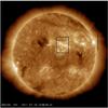 |
Fig. 1 Fe xii 193 Å AIA image. The area observed on the disk by EIS is outlined by the black box. The black perpendicular line on the right side of the image represents the EIS slit position off-limb. Only the bottom quarter of the off-limb slit is used for data analysis. The area scanned by SUMER is shown in a closer view in Fig. 4. |
2.1. SUMER data: Doppler shift of Mg x
Since 1995 the normal incidence spectrograph, SUMER, operates between 450 Å to 1610 Å wavelength range. This powerful UV instrument is designed to investigate the bulk motions of plasma in the chromosphere, transition region, and low corona. The spatial resolution of SUMER across and along the slit is 1 arcsec and 2 arcsec, respectively. The spectral scale (≈ 43 mÅ/pix at 1240 Å in the first order of diffraction, Wilhelm et al. 1997; Lemaire et al. 1997) is accurate enough2 to measure the Doppler shift of lines down to 1 km s-1. Corrections for wavelength-reversion, dead-time, flat-field, and detector electronicdistortion are applied to SUMER raw spectral images.
We use SUMER to measure the absolute Doppler shift of one coronal line (Mg x 625 Å) observed in the second order of diffraction around 1250 Å. SUMER does not have an on-board calibration source, hence we obtain the wavelength scale by using a set of chromospheric lines from neutrals and singly ionized atoms (for instance, C i lines with formation temperatures of 10 000 K.). These lines are known to have negligible or small average Doppler shifts (Hassler et al. 1991; Samain 1991). The wavelength calibration has three main steps: identifying the lines by using a preliminarily wavelength scale, fitting the Gaussian curves to the spectral lines to find the exact pixel position of the lines, performing a polynomial fit to obtain the dispersion relation.
The SUMER data that we have used here consist of a sit-and-stare3 sequence near disk center over a moss area within active region NOAA 11243. The acquired spectra (1245 Å to 1255 Å containing the Mg x 625 Å line, log T/ [K] = 6.00) are obtained by exposing for 75 s through the 1 × 300 arcsec2 slit. The sequence consists of 48 spectra and results in a small, 10 arcsec wide, drift scan by solar rotation.
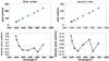 |
Fig. 2 Left column: top panel shows the first order polynomial fit to pixel positions versus rest wavelengths of 8 suitable reference lines around the Mg x 625 Å line. Lower panel represents the residuals of the fitting. The residuals are large, up to 0.6 pixels (~6 km s-1). Right column: top and lower panels represent a second order polynomial fit to pixel positions versus rest wavelengths and the residuals of the fitting, respectively. The residuals lie within ± 0.1 pixels (about 1 km s-1). |
We have checked the data to be sure that there are no significant instrumental drifts in the position of the spectral lines (either along the slit or as a function of time across the raster). A high signal to noise spectrum is obtained by averaging over the region of interest. Then, by choosing eight suitable reference lines (from relatively strong and unblended lines of neutral or singly ionized atoms) we have performed the wavelength calibration. A linear fit of their positions in pixels versus their laboratory wavelengths results in residuals of less than ± 0.6 pixels (see left column of Fig. 2). The residuals clearly show the need for a second-order polynomial fit that leaves residuals of ± 0.1 pixels (less than 2 km s-1). This is demonstrated in right column of Fig. 2. Dadashi et al. (2011) also used a second order polynomial fit to obtain the velocity of the same line over a quiet Sun area. We believe the need for the higher order fit comes from residual errors in the correction of the electronic distortion of the detector image.
To obtain the Doppler shift map of the Mg x 625 Å line, we have used 624.967 Å as rest wavelength. This is the average between the values of (624.965 ± 0.003) Å given by Dammasch et al. (1999) and (624.968 ± 0.007) Å given by Peter & Judge (1999). The reasons for this selection of the above rest wavelength are described in detail in Dadashi et al. (2011).
2.2. EIS data: analysis and co-alignment
The EIS instrument produces high-resolution stigmatic spectra in the wavelength ranges of 170 to 210 Å and 250 to 290 Å. The instrument has 1 arcsec spatial pixels and 0.0223 Å spectral pixels. More details are given in Culhane et al. (2007) and Korendyke et al. (2006).
EIS data consists of one raster scan (1 arcsec step size and 30 s exposure time) of the active region taken nearly simultaneously to the SUMER data, followed by one sit-and-stare sequence taken above the limb. Both observations were obtained using the 1 arcsec wide slit. The area of study (NOAA active region 11243) is shown in different wavelength bands of AIA/SDO in Fig. 3. The over-plotted yellow box on each panel of this figure shows the moss area that we had studied here.
 |
Fig. 3 The NOAA active region 11243 is shown in different wavelength bands of AIA/SDO (top panels). The images are taken on 4th July 2011 at 17:00 UTC. The yellow boxes show the moss area studied in this work. Lower panels are blow ups of the corresponding yellow boxes. |
The eis_prep.pro routine, which is the standard EIS data reduction routine available in the SolarSoft (SSW) package, is used. This routine subtracts the dark current, removes the cosmic rays and hot pixels, and does radiometric calibration. The slit tilt and orbital variation effects are removed from the data by using the SSW eis_wave_corr.pro routine. The orbital variation caused by the thermal effects on the instrument does not play an important role in our study, since the technique we employ is based on the measurement of the line separations (the distance between the line of which we want to measure the shift and a reference line), a quantity that does not change during the relatively short duration of our observations (for further details see Dadashi et al. 2011).
After removing the offset between the SW and LW detectors, we co-align the two instruments (SUMER and EIS) by using a pair of radiance maps obtained in lines formed at similar temperatures: Mg x 625 Å (SUMER) and Fe x 184 Å (EIS). The left panel of Fig. 4 shows the position of the SUMER slit at the beginning of the drift scan over-plotted on the EIS Fe x 184 Å image raster. The SUMER slit crosses the moss area that we have studied in this paper. The right panel of Fig. 4 is a blow-up of the pink box shown in the left panel. The area scanned by SUMER is placed between red and yellow inclined lines. Intensity contours of Mg x 625 Å plotted on top of the intensity map of Fe x 184 Å allow us to co-align the image with an accuracy of roughly 1 arcsec.
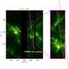 |
Fig. 4 Left panel: the position of the SUMER slit at the start of the drift scan over-plotted on the EIS Fe x 184 Å intensity image raster. The SUMER slit crosses the moss area that we have studied in this paper. Right panel: blow up of the pink box in the left panel. Intensity contours of Mg x 625 Å are plotted on top of the intensity map of the Fe x 184 Å line. |
2.3. Method of measuring absolute Doppler shifts
Since there are no suitable cool chromospheric lines in the EIS wavelength range, it is not possible to use the same calibration technique as with SUMER.
One of the alternatives is to measure “relative” Doppler shifts of hot coronal lines by comparing to observations of quiet Sun areas that are present in the same raster scan containing the target active region. To obtain “absolute” Doppler shifts with this technique, Young et al. (2012) have used the average absolute velocities in the quiet Sun measured by Peter & Judge (1999) using SUMER spectra. However, there is some degree of uncertainty and arbitrariness in identifying what is quiet Sun near an active region, leading to a substantial uncertainty of the absolute velocity.
Dadashi et al. (2011) have introduced a novel technique to obtain “absolute” Doppler shifts of hot coronal lines using simultaneous observation of EIS and SUMER. The technique is based on two important assumptions:
-
First, above the limb of quiet regions without obvious structures,the spectral lines have, on average, no Doppler shift because themotions out of the plane of sky cancel out on average.
-
Second, Mg x 625 Å (SUMER) and Fe x 184 Å (EIS) lines, which have similar formation temperature, have the same average Doppler shift in the common area of study4.
Following Dadashi et al. (2011), we consider the EIS Fe x 184 Å line as the reference line and obtain all other coronal line velocities respect to this line. 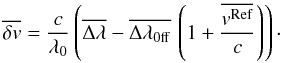 (1)Then, the absolute Doppler shifts are obtained as
  (2)where
  and
and  are the relative (to Fe x) and absolute average Doppler shift of each line and
  is the average Doppler shift of the Mg x line measured by SUMER (see Fig. 5), assumed to be equal to that of the reference line (Fe x). c and λ0 are the speed of light in vacuum and the rest wavelength of the line of which we want to measure the shift. Since λ0 is not used to calculate the shift of the spectral line due to the Doppler effect, it does not need to be known with high accuracy.
 and
and  are the average of the distribution of wavelength separation of the two lines (the line of which we want to measure the shift and the reference line) on disk and off-limb, respectively. In this work we use this technique to measure the absolute Doppler shift of hot coronal lines in the moss region of NOAA active region 11243. To have a higher signal-to-noise ratio, before fitting the line profiles, we have binned the on-disk spectra over two raster positions and over two pixels along the slit (2 × 2 binning). In the case of off-limb spectra we have used a binning of 3 × 20 (3 in solar X and 20 in solar Y direction).
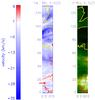 |
Fig. 5 Intensity and velocity maps of Mg x 625 Å obtained by the sit-and-stared SUMER observations. Contours of Fe x 184 Å are plotted on both maps. The area that is marked by the red arrow corresponds to region b in the moss area (defined in the left panel of Fig. 6). The average Doppler velocity of Mg x 625 Å is of −6.6 km s-1 inside region b and of (− 5.50 ± 0.55) km s-1 over the whole area shown here. |
This way, maps of relative Doppler shift were first obtained for Fe xi 188 Å, Fe xii 192 Å, Fe xiii 202 Å, Fe xiv 270 Å, and Fe xv 284 Å lines. The absolute Doppler shift map of Fe x 184 Å was obtained by imposing as rest wavelength a value that gives the same velocity pattern as Mg x 625 Å in the common observed area. After this, all relative Doppler maps were easily converted into absolute Doppler maps.
2.4. Moss identification
Figure 6 shows three different contours of the intensity of the Fe xii 192 Å line dividing the whole area of study into 4 different regions. We consider the middle intensity contour as a threshold to identify moss (regions a and b together, as marked in the left panel of Fig. 6).
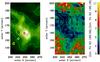 |
Fig. 6 Left panel: intensity map of Fe xii 192 Å. Right panel: the intensity ratio of Fe xii 192 Å and Fe xii 195.2 Å lines. Smaller ratios correspond to higher electron densities. The identified moss area (regions a and b) lie in the regions with higher density, as expected. Contours of intensity of the Fe xii 192 Å line are plotted on both maps. |
The intensity ratio of Fe xii 192.39 Å and Fe xii 195.18 Å is density-sensitive. Using the CHIANTI atomic database (Landi et al. 2012), we have derived the intensity ratio of these two lines as a function of density (Fig. 7). Smaller intensity ratios correspond to higher densities. Right panel of Fig. 6 shows the map of the intensity ratio of the above Fe xii lines.
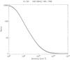 |
Fig. 7 Intensity ratio of Fe xii 192 Å and Fe xii 195.18 Å lines as a function of density. Smaller intensity ratios correspond to higher densities. |
Brighter intensity contours of Fe xii 192.39 Å line, which determine the moss region, are plotted on both maps. The identified moss region is characterized by higher density, as expected. The average electron density for regions a, b, c, and d are listed in Table 1. The average moss density (average of regions a and b) is about 6.6 × 109 cm-3, which is a bit larger than 4.2 to 5.3 × 109 cm-3 reported by Fletcher & de Pontieu (1999). On the other hand, Tripathi et al. (2010a) obtained larger electron densities of about 10 to 30 × 109 cm-3 using the Fe xii 195.12 Å and 186.88 line ratio. However, we should consider that the densities obtained by Fe xii lines are overestimated in high density regions. The new Fe xii calculations by Del Zanna et al. (2012) show that there was some problem with the atomic data which has now been resolved.
3. Result and discussion
Using the technique introduced by Dadashi et al. (2011), and summarized in Section 2.3, we have obtained the line of sight Doppler shifts of hot coronal lines in a moss area of the active region NOAA 11243. In the first step of our study, we have defined the moss area by intensity contours of Fe xii 192 Å. Based on these contours, four different areas are defined in that region (left panel of Fig. 6). Table 2 lists the Doppler shift values for each of these regions with the corresponding uncertainties. Positive and negative values of velocity represent downflows (red shifts) and upflows (blue shifts), respectively.
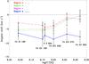 |
Fig. 8 Average Doppler shift of hot coronal lines in different regions defined in the left panel of Fig. 7, plotted as a function of formation temperature. Fe xii and S x have nearly the same formation temperature, but are plotted a bit separated for better readability. Positive and negative values of velocity represent downflows (red shifts) and upflows (blue shifts), respectively. |
The error reported in this Table  is obtained by error propagation analysis of Eqs. (1) and (2). The error on
  is given by the width σ of the off-limb line-separation distribution. Since the on-disk line separation distribution is also broadened by the different Doppler speeds characterizing the two lines at different temperatures, the error for
  is assumed to be equal to that off-limb. This leads to the same error for a given line in all different regions on disk.
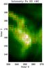 |
Fig. 9 Ten different small square areas selected to study the Doppler velocities therein, overplotted on a map of Fe xii 192 Å intensity. Green contours are intensity contours of Fe xii 192 Å. |
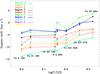 |
Fig. 10 Doppler shift as a function of temperature for the ten boxes defined in Fig. 9. Fe xii and S x have the same formation temperature but are plotted a bit separated for better readability. |
Figure 8 shows the average Doppler shift for the four regions defined by intensity contours of the Fe xii 192 Å as a function of temperature. The Doppler shifts of the lines in the temperature range from 1 to 1.6 MK over regions a, b, and c show constant blue shifts or upward motions of about 5 km s-1. For hotter lines the upward motions decrease down to about 1 km s-1 for Fe xv. Region a, which corresponds to the highest electron densities and intensities of the Fe xii 192 Å line, shows a somewhat smaller blue shift than the other regions for temperatures below 1.8 MK. Region d, that has the smallest intensity and density values, shows almost constant and stronger blue shift of about 8 km s-1, in the temperature range from 1 to 2 MK.
For hotter lines (1.6 to 2 MK) there is almost no prevalent motion in regions a, b, and c (0 to 2 km s-1, with velocities never diverging by more than 2σ from zero). Region d at the same temperature shows strong blue shift.
To have a better understanding of the behavior, we have selected ten small boxes at different locations of the area of interest (shown in Fig. 9) and calculated the average absolute Doppler shifts inside each box. Figure 10 displays the average absolute Doppler shifts of different ions as a function of their formation temperatures in the ten selected areas.
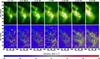 |
Fig. 11 Intensity (upper panels) and velocity maps (lower panels) for Different ions with different formation temperatures. Green contours are intensity contours of Fe xii 192 Å plotted on top of intensity (top row) and velocity maps (bottom row) of different ions. Yellow contours on velocity maps outline red shifted pixels. Red contour is the brightest area which is common in both EIS and SUMER field of views and is used for velocity calibration. |
The same general behavior of velocity is observed with respect to temperature in all regions. Doppler shifts are essentially constant up to temperatures of about 1.6 MK. Above this value, upward velocities decrease and almost stop at a temperature of about 2 MK except for the loop legs and the parts of the moss with lower electron densities (e.g. regions 1, 2, 3, 9, and 10). The inner (brighter and denser) part of the moss shows smaller upflows (regions 4 and 5). In contrast, regions 1, 2 and 8, 9, which are on the legs of the hot coronal loops (as suggested also by magnetic field extrapolations, see Fig. 12), show larger blue shift (upward motions) of about 10 km s-1 between 1 MK and 1.6 MK. This suggest that as the plasma rises higher along the loop leg, it accelerates. This conclusion is further illustrated by region 10, which lies further up in the loop leg and is associated with higher upflows of about 13 to 14 km s-1). In all regions, colder lines sense stronger upflows (the colder, the more shifted to the blue).
Hotter lines like Fe xiv 270 Å and Fe xv 284 Å in the brighter and denser part of moss reveal no significant motions (the only exception is region 5 that shows a small red shift (downward motion) of about 3 km s-1 at this temperature). The intensity and corresponding Doppler shift maps of all these hot coronal lines are plotted in Fig. 11. The red shifted area of Fe xiv and Fe xv lies within the yellow contours overplotted on the corresponding velocity maps.
Our results for Fe xii are based on the unblended Fe xii line at 192 Å. However, we have also obtained the velocity from the Fe xii 195.120 line which is one of the brightest lines recorded by EIS. This line is blended by Fe xii 195.180 Å in its red wing. The density sensitive ratio, 195.180/195.120, increases with increasing density. Considering both components, performing a double Gaussian fit will result in redder velocities than the other unblended Fe xii lines5 (Young et al. 2009). Here we find that considering a double Gaussian profile for Fe xii 195 Å on average results in a velocity redder than Fe xii 192 Å by about 2.2 km s-1.
To have a more precise idea about the orientation of the hot coronal loops, we have extrapolated the photospheric field into the solar corona by using photospheric vector magnetograms obtained by the Helioseismic and Magnetic Imager (HMI, Schou et al. 2012) aboard Solar Dynamics Observatory (SDO). The nonlinear force-free coronal magnetic field extrapolation technique used here is described in detail by Wiegelmann et al. (2012). Figure 12 shows the magnetic field lines plotted over an AIA/SDO image taken at 17:00 UTC, which lies within the time frame of our study. The field of view for applying nonlinear coronal magnetic field extrapolation (the whole window of Fig. 12) is chosen in order to fulfill consistency criteria:
-
The vector magnetogram should be almost perfectly fluxbalanced.
-
The field of view should be large enough to cover weak field surrounding of the target active region.
The field lines shown in Fig. 12 better reveal the prevailing direction of the hot loops than can be seen in the 211 and 335 AIA channels. Note that the loops emerging from the moss extend away from it in two directions. These are the short loops extending North-East from the upper part of the moss. These correspond to the loops well visible in Fe xiv and Fe xv, whose legs are sampled by boxes 1, 2, 8, 9, and 10 in Fig. 9. The results of the magnetic field extrapolation show another set of loops which is directed the South-East starting from the moss (more visible in cooler lines like Fe ix 171 Å). Thus, the Fe xiv and Fe xv red shifted regions visible in Fig. 11 (outlined by the yellow contours) appear located in the areas free of line-of-sight contamination from plasma higher up along the loop legs. Since the emission from the loop legs is clearly blue shifted, we may speculate that the near zero blue shifts observed over the moss may actually be a combination of red shift at the footpoint and blue shift along the loops. Both red and blue shifts are too small to leave a signature in the line profile sufficiently strong to disentangle the two velocity components in a single line profile at the EIS spectral resolution. However, the possibility that the red shifted region seen in Fe xv is due to an independent phenomenon, cannot be entirely excluded.
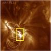 |
Fig. 12 Magnetic field lines extrapolated from photospheric field and plotted over Fe xii 193 Å image of AIA/SDO. Red contours show positive and blue and green contours show negative polarities. The yellow frame represents the region of the moss study in this work. |
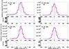 |
Fig. 13 Spectral profiles of Fe xii, Fe xiii, Fe xiv, and Fe xv obtained over region 4 (defined in Fig. 9). |
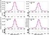 |
Fig. 14 Spectral profiles of Fe xii, Fe xiii, Fe xiv, and Fe xv obtained over region 5 (defined in Fig. 9). |
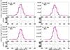 |
Fig. 15 Spectral profiles of Fe xii, Fe xiii, Fe xiv, and Fe xv obtained over region 10 (defined in Fig. 9). |
Impulsive heating models that consider a group of unresolved strands heated by periodic events like nanoflares, predict red shift (downward motion) on both legs of the loops in ~1 MK lines and more complex profiles with an extended blue wing in very hot lines such as Fe xvii (Klimchuk 2006; Patsourakos & Klimchuk 2006).
Our Doppler shift measurements inside the moss region do not show the predicted red shift of ~1 MK lines and the increasing blue shift of lines at increasingly higher temperatures, but rather the opposite. We clearly see blue shifted emission in lines formed between 1 and 1.6 MK and almost zero velocity at the Fe xv formation temperature. Moreover, we have studied the line profiles associated with some of these ten regions to look for possible asymmetries. Figures 13 to 15 show the spectral line profiles for Fe xii 192 Å, Fe xiii 202 Å, Fe xiv 270 Å, and Fe xv 284 Å over the selected regions 4, 5, and 10, respectively. A single Gaussian fit is performed on all line profiles. Residuals of each fit are also plotted right under the panel with the line profile.
The spectral profiles seem to be well represented by a Gaussian and no specific asymmetry is detected (residuals are less than 2 to 3% of the amplitudes of the line profiles). Fe xiv 270 Å and Fe xv 284 Å line profiles seem to be weakly blended with Mg vi 270.394 Å and Al ix 284.015 Å in their blue wings (the small bumps in the residual plots). After taking out the effect of these blends, all line profiles are highly symmetric (see also Tripathi et al., in prep.) If profiles with extended blue wings are actually present at the footpoints of hot loops, they are only observable in lines much hotter that Fe xv.
Measurements of density and thermal properties of moss observed by EIS have shown no significant change over several hours (Tripathi et al. 2010a). This leads the authors to suggest that the heating of the hot coronal loops associated to the moss might be quasi-steady. Brooks & Warren (2009) have shown that the amount and variability of shifts and widths of coronal lines is small and appears consistent with steady heating models. However, we note that variability of density, flows and line widths were studied on a spatially averaged region and any small scale variations may get averaged out. Steady heating models of perfectly symmetric coronal loops predict no bulk motions since the conductive flux from the corona is balanced by radiative cooling (Mariska & Boris 1983; Klimchuk et al. 2010). Impulsive heating, on the other hand, predicts definite plasma flows, which are temperature dependent. The relationship between velocity and temperature after spatial averaging may not be straight forward, as different strands may be evolving completely independently and providing mixed observational signatures.
The near absence of Doppler shifts in the hotter lines (Fe xiv and Fe xv) and, in general, the absence of red shifted emission in the observed moss region, along with the observed symmetric line profiles, seems to be consistent with quasi-steady heating of nonsymmetric loops. Steady heating driven by pressure difference between the footpoints of the loops predicts the flows to be accelerated with height. For nonsymmetric loops, this effect will produce siphon-like flows in which one footpoint will be red shifted and the other would be blue shifted. Unfortunately, we cannot check and compare the flows at the other footpoint of these loops. In fact, due to the fact that the Hinode spacecraft suffered from seasonal eclipses at that time of the year, the other footpoint is missing in the EIS image raster (Fig. 4).
In support of quasi-steady heating of hot loops, we have found the Doppler shift to increase as we go higher in the loop leg (Figs. 9 and 10). However, observations of a larger sample of moss regions in lines covering higher temperatures than Fe xv would be necessary to consolidate our findings.
4. Summary
-
By combining SUMER and EIS data, with a new technique de-veloped by Dadashi et al. (2011),we have measured the absolute Doppler shift of hot coronal lines(Fe x 184 Å,Fe xi 188 Å,Fe xii 192 Å,Fe xiii 202 Å,Fe xiv 270 Å,and Fe xv 284 Å)in the moss of an active region.
-
The moss is identified as the region where Fe xii 192 Å intensity corresponds to electron densities above about 6.6 × 109 cm-3.
-
The inner (brighter and denser) part of the moss area shows roughly a constant blue shift (upward motions) of 5 km s-1 in the temperature range of 1 MK to 1.6 MK. For hotter lines the blue shift decreases, down to 1 km s-1 for Fe xv 284 Å. Absolute Doppler shift maps are obtained using the Dadashi et al. (2011) technique. The general dependence of the velocity on temperature seems to be the same everywhere in the map. In all regions, the colder the line the stronger the blue shift.
-
In general, the inner (brighter and denser) part of the moss shows smaller blue shifts, whereas the legs of hot coronal loops with footpoints in the moss, show larger blue shift.
-
Our velocity measurements inside the moss region do not show the red shifts predicted by the impulsive loop heating model (Klimchuk 2006; Patsourakos & Klimchuk 2006). Also, we have found the line profiles to be highly symmetric, which is in contrast with the predictions of impulsive heating models.
-
The near absence of motions seen in the hotter lines and, in general, the absence of red shifted emission in the observed moss region, as well as the observed symmetric line profiles, and higher velocities in higher parts of the loop legs seem to be consistent with quasi-steady heating models for nonsymmetric loops.
 , where n, v, A, and s are density, velocity, cross section, and length coordinate along the 1D loop, respectively.
In case of high signal to noise ratios.
The slit stays fixed in space and let the Sun rotates beneath.
Reasons are described in Dadashi et al. (2011).
Acknowledgments
The SUMER project is financially supported by DLR, CNES, NASA, and the ESA PRODEX programme (Swiss contribution). SoHO is a mission of international cooperation between ESA and NASA. Hinode is a Japanese mission developed and launched by ISAS/JAXA, collaborating with NAOJ as a domestic partner, and NASA and STFC (UK) as international partners. Scientific operation of the Hinode mission is conducted by the Hinode science team organized at ISAS/JAXA. This team mainly consists of scientists from institutes in the partner countries. Support for the post-launch operation is provided by JAXA and NAOJ (Japan), STFC (U.K.), NASA, ESA, and NSC (Norway). Data are courtesy of NASA/SDO and the AIA and HMI science teams. This work has been partially supported by WCU grant No. R31-10016 funded by the Korean Ministry of Education, Science and Technology. N.D. acknowledges a PhD fellowship of the International Max Planck Research School on Physical Processes in the Solar System and Beyond. D.T. would like to thank MPS for supporting his travel and providing excellent hospitality.
References
- Antiochos, S. K., Karpen, J. T., DeLuca, E. E., Golub, L., & Hamilton, P. 2003, ApJ, 590, 547 [NASA ADS] [CrossRef] [Google Scholar]
- Aschwanden, M. J. 2004, Physics of the Solar Corona. An Introduction (Praxis Publishing Ltd) [Google Scholar]
- Berger, T. E., de Pontieu, B., Fletcher, L., et al. 1999, Sol. Phys., 190, 409 [NASA ADS] [CrossRef] [Google Scholar]
- Boris, J. P., & Mariska, J. T. 1982, ApJ, 258, L49 [NASA ADS] [CrossRef] [Google Scholar]
- Bradshaw, S. J., & Klimchuk, J. A. 2011, ApJS, 194, 26 [NASA ADS] [CrossRef] [Google Scholar]
- Brooks, D. H., & Warren, H. P. 2009, ApJ, 703, L10 [NASA ADS] [CrossRef] [Google Scholar]
- Brooks, D. H., Ugarte-Urra, I., & Warren, H. P. 2008, ApJ, 689, L77 [NASA ADS] [CrossRef] [Google Scholar]
- Cargill, P. J. 1994, ApJ, 422, 381 [Google Scholar]
- Craig, I. J. D., & McClymont, A. N. 1986, ApJ, 307, 367 [NASA ADS] [CrossRef] [Google Scholar]
- Culhane, J. L., Harra, L. K., James, A. M., et al. 2007, Sol. Phys., 243, 19 [Google Scholar]
- Dadashi, N., Teriaca, L., & Solanki, S. K. 2011, A&A, 534, A90 [NASA ADS] [CrossRef] [EDP Sciences] [Google Scholar]
- Dammasch, I. E., Hassler, D. M., Wilhelm, K., & Curdt, W. 1999, in 8th SOHO Workshop: Plasma Dynamics and Diagnostics in the Solar Transition Region and Corona, eds. J.-C. Vial, & B. Kaldeich-Schü, ESA SP, 446, 263 [Google Scholar]
- Del Zanna, G. 2008, A&A, 481, L49 [NASA ADS] [CrossRef] [EDP Sciences] [Google Scholar]
- Del Zanna, G., Storey, P. J., Badnell, N. R., & Mason, H. E. 2012, A&A, 543, A139 [NASA ADS] [CrossRef] [EDP Sciences] [Google Scholar]
- Doschek, G. A., Mariska, J. T., Warren, H. P., et al. 2007, ApJ, 667, L109 [NASA ADS] [CrossRef] [Google Scholar]
- Doschek, G. A., Warren, H. P., Mariska, J. T., et al. 2008, ApJ, 686, 1362 [NASA ADS] [CrossRef] [Google Scholar]
- Fletcher, L., & de Pontieu, B. 1999, ApJ, 520, L135 [NASA ADS] [CrossRef] [Google Scholar]
- Hara, H., Watanabe, T., Harra, L. K., et al. 2008, ApJ, 678, L67 [NASA ADS] [CrossRef] [Google Scholar]
- Hassler, D. M., Rottman, G. J., & Orrall, F. Q. 1991, Adv. Space Res., 11, 141 [NASA ADS] [CrossRef] [Google Scholar]
- Klimchuk, J. A. 2006, Sol. Phys., 234, 41 [NASA ADS] [CrossRef] [Google Scholar]
- Klimchuk, J. A. 2009, in The Second Hinode Science Meeting: Beyond Discovery-Toward Understanding, eds. B. Lites, M. Cheung, T. Magara, J. Mariska, & K. Reeves, ASP Conf. Ser., 415, 221 [Google Scholar]
- Klimchuk, J. A., Karpen, J. T., & Antiochos, S. K. 2010, ApJ, 714, 1239 [NASA ADS] [CrossRef] [Google Scholar]
- Korendyke, C. M., Brown, C. M., Thomas, R. J., et al. 2006, Appl. Opt., 45, 8674 [NASA ADS] [CrossRef] [Google Scholar]
- Landi, E., Del Zanna, G., Young, P. R., Dere, K. P., & Mason, H. E. 2012, ApJ, 744, 99 [NASA ADS] [CrossRef] [Google Scholar]
- Lemaire, P., Wilhelm, K., Curdt, W., et al. 1997, Sol. Phys., 170, 105 [NASA ADS] [CrossRef] [Google Scholar]
- Lemen, J. R., Title, A. M., Akin, D. J., et al. 2012, Sol. Phys., 275, 17 [NASA ADS] [CrossRef] [Google Scholar]
- Mariska, J. T., & Boris, J. P. 1983, ApJ, 267, 409 [NASA ADS] [CrossRef] [Google Scholar]
- Noci, G. 1981, Sol. Phys., 69, 63 [NASA ADS] [CrossRef] [Google Scholar]
- Orlando, S., Peres, G., & Serio, S. 1995, ApJ, 300, 549 [Google Scholar]
- Patsourakos, S., & Klimchuk, J. A. 2006, ApJ, 647, 1452 [NASA ADS] [CrossRef] [Google Scholar]
- Patsourakos, S., Klimchuk, J. A., & MacNeice, P. J. 2004, ApJ, 603, 322 [NASA ADS] [CrossRef] [Google Scholar]
- Peter, H., & Judge, P. G. 1999, ApJ, 522, 1148 [NASA ADS] [CrossRef] [Google Scholar]
- Samain, D. 1991, A&A, 244, 217 [NASA ADS] [Google Scholar]
- Schou, J., Scherrer, P. H., Bush, R. I., et al. 2012, Sol. Phys., 275, 229 [Google Scholar]
- Tripathi, D., Mason, H. E., Young, P. R., & Del Zanna, G. 2008, ApJ, 481, L53 [Google Scholar]
- Tripathi, D., Mason, H. E., Dwivedi, B. N., del Zanna, G., & Young, P. R. 2009, ApJ, 694, 1256 [NASA ADS] [CrossRef] [Google Scholar]
- Tripathi, D., Mason, H. E., Del Zanna, G., & Young, P. R. 2010a, ApJ, 518, A42 [Google Scholar]
- Tripathi, D., Mason, H. E., & Klimchuk, J. A. 2010b, ApJ, 723, 713 [NASA ADS] [CrossRef] [Google Scholar]
- Tripathi, D., Klimchuk, J. A., & Mason, H. E. 2011, ApJ, 740, 111 [NASA ADS] [CrossRef] [Google Scholar]
- Tripathi, D., Mason, H. E., & Klimchuk, J. A. 2012, ApJ, 753, 37 [NASA ADS] [CrossRef] [Google Scholar]
- Ugarte-Urra, I., Warren, H. P., & Brooks, D. H. 2009, ApJ, 695, 642 [NASA ADS] [CrossRef] [Google Scholar]
- Viall, N. M., Klimchuk, J. A., & Goddard Space Flight Center, N. 2012, ApJ, 753, 35 [NASA ADS] [CrossRef] [Google Scholar]
- Warren, H. P., Winebarger, A. R., & Mariska, J. T. 2003, ApJ, 593, 1174 [NASA ADS] [CrossRef] [Google Scholar]
- Warren, H. P., Winebarger, A. R., Mariska, J. T., Doschek, G. A., & Hara, H. 2008, ApJ, 677, 1395 [NASA ADS] [CrossRef] [Google Scholar]
- Warren, H. P., Winebarger, A. R., & Brooks, D. H. 2010, ApJ, 711, 228 [NASA ADS] [CrossRef] [Google Scholar]
- Wiegelmann, T., Thalmann, J. K., Inhester, B., et al. 2012, Sol. Phys., 67 [Google Scholar]
- Wilhelm, K., Curdt, W., Marsch, E., et al. 1995, Sol. Phys., 162, 189 [NASA ADS] [CrossRef] [Google Scholar]
- Wilhelm, K., Lemaire, P., Curdt, W., et al. 1997, Sol. Phys., 170, 75 [NASA ADS] [CrossRef] [Google Scholar]
- Winebarger, A. R., Warren, H., van Ballegooijen, A., DeLuca, E. E., & Golub, L. 2002, ApJ, 567, L89 [NASA ADS] [CrossRef] [Google Scholar]
- Winebarger, A. R., Warren, H. P., & Falconer, D. A. 2008, ApJ, 676, 672 [NASA ADS] [CrossRef] [Google Scholar]
- Winebarger, A. R., Schmelz, J. T., Warren, H. P., Saar, S. H., & Kashyap, V. L. 2011, ApJ, 740, 2 [NASA ADS] [CrossRef] [Google Scholar]
- Winebarger, A., Tripathi, D., Mason, H. E., & Del Zanna, G. 2012, ApJ, submitted [Google Scholar]
- Young, P. R., Watanabe, T., Hara, H., & Mariska, J. T. 2009, A&A, 495, 587 [NASA ADS] [CrossRef] [EDP Sciences] [Google Scholar]
- Young, P. R., O’Dwyer, B., & Mason, H. E. 2012, ApJ, 744, 14 [NASA ADS] [CrossRef] [Google Scholar]
All Tables
All Figures
|
Fig. 1 Fe xii 193 Å AIA image. The area observed on the disk by EIS is outlined by the black box. The black perpendicular line on the right side of the image represents the EIS slit position off-limb. Only the bottom quarter of the off-limb slit is used for data analysis. The area scanned by SUMER is shown in a closer view in Fig. 4. |
| In the text | |
|
Fig. 2 Left column: top panel shows the first order polynomial fit to pixel positions versus rest wavelengths of 8 suitable reference lines around the Mg x 625 Å line. Lower panel represents the residuals of the fitting. The residuals are large, up to 0.6 pixels (~6 km s-1). Right column: top and lower panels represent a second order polynomial fit to pixel positions versus rest wavelengths and the residuals of the fitting, respectively. The residuals lie within ± 0.1 pixels (about 1 km s-1). |
| In the text | |
|
Fig. 3 The NOAA active region 11243 is shown in different wavelength bands of AIA/SDO (top panels). The images are taken on 4th July 2011 at 17:00 UTC. The yellow boxes show the moss area studied in this work. Lower panels are blow ups of the corresponding yellow boxes. |
| In the text | |
|
Fig. 4 Left panel: the position of the SUMER slit at the start of the drift scan over-plotted on the EIS Fe x 184 Å intensity image raster. The SUMER slit crosses the moss area that we have studied in this paper. Right panel: blow up of the pink box in the left panel. Intensity contours of Mg x 625 Å are plotted on top of the intensity map of the Fe x 184 Å line. |
| In the text | |
|
Fig. 5 Intensity and velocity maps of Mg x 625 Å obtained by the sit-and-stared SUMER observations. Contours of Fe x 184 Å are plotted on both maps. The area that is marked by the red arrow corresponds to region b in the moss area (defined in the left panel of Fig. 6). The average Doppler velocity of Mg x 625 Å is of −6.6 km s-1 inside region b and of (− 5.50 ± 0.55) km s-1 over the whole area shown here. |
| In the text | |
|
Fig. 6 Left panel: intensity map of Fe xii 192 Å. Right panel: the intensity ratio of Fe xii 192 Å and Fe xii 195.2 Å lines. Smaller ratios correspond to higher electron densities. The identified moss area (regions a and b) lie in the regions with higher density, as expected. Contours of intensity of the Fe xii 192 Å line are plotted on both maps. |
| In the text | |
|
Fig. 7 Intensity ratio of Fe xii 192 Å and Fe xii 195.18 Å lines as a function of density. Smaller intensity ratios correspond to higher densities. |
| In the text | |
|
Fig. 8 Average Doppler shift of hot coronal lines in different regions defined in the left panel of Fig. 7, plotted as a function of formation temperature. Fe xii and S x have nearly the same formation temperature, but are plotted a bit separated for better readability. Positive and negative values of velocity represent downflows (red shifts) and upflows (blue shifts), respectively. |
| In the text | |
|
Fig. 9 Ten different small square areas selected to study the Doppler velocities therein, overplotted on a map of Fe xii 192 Å intensity. Green contours are intensity contours of Fe xii 192 Å. |
| In the text | |
|
Fig. 10 Doppler shift as a function of temperature for the ten boxes defined in Fig. 9. Fe xii and S x have the same formation temperature but are plotted a bit separated for better readability. |
| In the text | |
|
Fig. 11 Intensity (upper panels) and velocity maps (lower panels) for Different ions with different formation temperatures. Green contours are intensity contours of Fe xii 192 Å plotted on top of intensity (top row) and velocity maps (bottom row) of different ions. Yellow contours on velocity maps outline red shifted pixels. Red contour is the brightest area which is common in both EIS and SUMER field of views and is used for velocity calibration. |
| In the text | |
|
Fig. 12 Magnetic field lines extrapolated from photospheric field and plotted over Fe xii 193 Å image of AIA/SDO. Red contours show positive and blue and green contours show negative polarities. The yellow frame represents the region of the moss study in this work. |
| In the text | |
|
Fig. 13 Spectral profiles of Fe xii, Fe xiii, Fe xiv, and Fe xv obtained over region 4 (defined in Fig. 9). |
| In the text | |
|
Fig. 14 Spectral profiles of Fe xii, Fe xiii, Fe xiv, and Fe xv obtained over region 5 (defined in Fig. 9). |
| In the text | |
|
Fig. 15 Spectral profiles of Fe xii, Fe xiii, Fe xiv, and Fe xv obtained over region 10 (defined in Fig. 9). |
| In the text | |
Current usage metrics show cumulative count of Article Views (full-text article views including HTML views, PDF and ePub downloads, according to the available data) and Abstracts Views on Vision4Press platform.
Data correspond to usage on the plateform after 2015. The current usage metrics is available 48-96 hours after online publication and is updated daily on week days.
Initial download of the metrics may take a while.