| Issue |
A&A
Volume 548, December 2012
|
|
|---|---|---|
| Article Number | A9 | |
| Number of page(s) | 20 | |
| Section | Numerical methods and codes | |
| DOI | https://doi.org/10.1051/0004-6361/201219992 | |
| Published online | 13 November 2012 | |
A study of simulated reionization histories with merger trees of HII regions
Observatoire Astronomique de Strasbourg, Université de Strasbourg, CNRS UMR
7550, 11 rue de l’Université,
67000
Strasbourg,
France
e-mail:
This email address is being protected from spambots. You need JavaScript enabled to view it.
Accepted: 11 July 2012Received: 24 September 2012
Abstract
Aims. We describe a new methodology for analyzing the reionization process in numerical simulations. The chronology and the geometry of reionization is investigated by the merger histories of individual HII regions.
Methods. From the merger tree of ionized patches, one can track the individual evolution of the regions properties, such as their size, the intensity of the percolation process by looking at the formation rate, the frequency of mergers, and the number of individual HII regions involved in the mergers. We applied the merger-tree technique to simulations of reionization with three different kinds of ionizing source models and two resolutions. Two of them use star particles as ionizing sources. In this case we compared two emissivity evolutions for the sources to reach the reionization at z ~ 6. As an alternative we built a semi-analytical model where the dark matter halos extracted from the density fields are assumed as ionizing sources.
Results. We then show how this methodology is a good candidate to quantify the impact of the adopted star formation on the history of the observed reionization. The semi-analytical model shows a homogeneous reionization history with local hierarchical growth steps for individual HII regions. On the other hand, autoconsistent models for star formation tend to present fewer regions, with a dominant region in size that governs the fusion process early in the reionization at the expense of the local reionizations. The differences are attenuated when the resolution of the simulation is increased.
Key words: dark ages, reionization, first stars / methods: numerical / radiative transfer
© ESO, 2012
1. Introduction
The first generation of stars appears after the period called the dark ages (between z ~ 1090 and z ~ 20), creating a multitude of distinct HII regions in the Universe. These regions eventually merge with other ionized regions, leading to a total reionization of the Universe. The diffusion of CMB photons on the electrons released during reionization (see e.g. Komatsu et al. 2009) and the absorption features in the spectra of high-redshift quasars (see e.g. Fan et al. 2006; Willott et al. 2007) suggest that the end of reionization occurred at z ~ 11−6, with an average neutral fraction of hydrogen between 10-4 and 10-6 (see Fan et al. 2006).
Many models (see e.g. Barkana & Loeb 2004; Furlanetto et al. 2004b; Zahn et al. 2007; Mesinger & Furlanetto 2007; Choudhury et al. 2009) and simulation techniques (Abel et al. 1999; Gnedin & Abel 2001; Razoumov et al. 2002; Iliev et al. 2006a; Trac & Cen 2007; Aubert & Teyssier 2008; Finlator et al. 2009a; Petkova & Springel 2009) have been proposed to investigate the impact of the radiative transfer on the reionization epoch. See Trac & Gnedin (2011) for a complete review of these models. In parallel, semi-analytic models have been developed (Barkana & Loeb 2004; Furlanetto et al. 2004b; Zahn et al. 2007; Mesinger & Furlanetto 2007; Choudhury et al. 2009), mostly based on the “excursion set formalism” method (Bond et al. 1991) where both the source distribution and ionization fields are derived from the density fields.
In this context, one challenge is to describe the geometry and the time sequence of the reionization since they will be influenced by, e.g., the formation rate of ionizing sources, the distribution of their formation sites, or the size and growth of HII regions. Aiming at this description, many theoretical studies have thus been conducted that focus on the overall evolution of physical fields, such as the ionized fraction or temperature (see e.g. Aubert & Teyssier 2010; Finlator et al. 2009b). Alternately, many groups have undertaken analyses to characterize this period but by focusing on the properties of individual HII regions (Iliev et al. 2006b; Zahn et al. 2007; McQuinn et al. 2007; Lee et al. 2008; Croft & Altay 2008; Shin et al. 2008; Friedrich et al. 2011).
With the current article, we also aim at investigating the chronology and geometry of the reionization through numerical simulations. In particular, we describe the process through the study of the merger process of HII regions, and for this purpose we track the individual histories of the ionized regions formed in numerical simulations. Using this point of view, we combine the analysis in terms of individual HII regions with the temporal evolution of overall fields. As a consequence, it leads to a local perspective with a set of histories of reionization, allowing their scatter to be studied throughout a cosmological volume. This will be an alternative approach to those already undertaken.
In this paper, we first focus on the procedure for separating the different HII regions and to track each of them along time. For this purpose, we follow many other investigations (Iliev et al. 2006b; Shin et al. 2008; Friedrich et al. 2011) by using a friends-of-friends algorithm (FOF) to characterize the different ionized regions. Then, to follow the HII regions’ properties with time or redshift, we built their merger tree. Using the merger tree and investigating its properties to infer the redshift evolution of the HII regions’ formation number, their size evolution, and their merger history, we suggest a new way to constrain the evolution of the reionization process.
We tested the method on three models for the ionizing sources in order to quantify their impact on the simulated reionization history. We also quantified the impact of the spatial resolution of the simulations on the history by performing simulations with sizes of 200 and 50 Mpc/h boxes. By comparing the resulting reionization histories, we show how different source prescriptions lead to different properties on the evolution of HII regions as reionization progresses.
This paper is organized as follows. In Sect. 2, we present the tools developed to investigate the history of the reionization in simulations such as the FOF algorithm and the merger tree of HII regions. In Sect. 3, we describe the properties of the simulations that we study. In Sect. 4, first, we present our results in terms of general quantities, such as the ionization fraction or the optical depth evolution. Then, in Sect. 5, we compare the different histories of each model enlightened with the merger tree methodology. We finally discuss these results and their limits in Sect. 6 and draw our conclusions.
2. Analyzing merger trees of HII regions
2.1. Rationale
Merger trees have been used for 20 years in, e.g., the theoretical studies of galaxy formation (see e.g. Lacey & Cole 1993; Kauffmann & White 1993). More recently, seminal works, such as Furlanetto et al. (2004a) and subsequent analytical and semi-analytical investigations have used excursion set formalisms to construct histories of HII regions during reionization. Even though it is strongly connected to these works, the current paper aims at using merger trees differently. The trees, which are extracted from simulations, are used as objects worthy of study for their own properties; in other words, we analyze the simulated HII region merger histories from the merger trees they produce. The latter is not a means to providing higher level prediction, such as statistics on the 21 cm signal, but it is itself a probe of the simulation properties. On a broader perspective, the methodology presented here could be compared to genus or skeleton calculations as a reproductive and quantitative means to discussing the simulated process. It is thus complementary to power spectra or the time evolution of average quantities, for instance. In practice, in addition to tracking individual HII regions, we are thus led to analyze the “graph” properties of tree-based data, as shown below, and to draw conclusions about the simulated physics. Hereafter, we briefly present our implementation of the classic FOF technique to identify HII regions and the procedure for building merger trees. Additional details of these classic tools can be found in the appendix.
2.2. FOF identification of HII regions
We have developed an FOF algorithm that is able to separate the different HII regions at a given instant in snapshots of simulations and allocate an identification number to them. The following description of this FOF method is similar to those in previous studies (Iliev et al. 2006b; Shin et al. 2008; Friedrich et al. 2011). The ionization state of the gas is sampled on a regular grid.
Firstly, we define the status of the box cells in terms of ionization fraction. The rule we adopted is that a cell is ionized if it has an ionization fraction x ≥ 0.5 (often used in other works e.g. Iliev et al. 2006b; Shin et al. 2008; Friedrich et al. 2011). An individual HII region is defined by an identification number (ID hereafter). Secondly, if a cell is ionized and has an ID, then all its ionized nearest neighbors belong to the same ionized region and thus share the same ID. Our definition of nearest neighbors is limited to six cells along the main directions. One single isolated cell is then considered as a single ionized region. More details about the FOF implementation can be found in Appendix A.
We have to note that the FOF procedure is not without caveats, so we could have adopted higher values for the ionization fraction threshold, for example. We can then imagine that HII regions would be more divided and more numerous with smaller sizes in this case, possibly leading to different reionization histories. In the appendix, we show that the statistics of the regions weakly depend on this specific value of the ionization threshold in the 0.3−0.9 range, except for the smallest regions with recombining episodes. The FOF technique can also connect distant regions with ionized bridges, an effect that might be undesirable. Alternately, we could have chosen other methods for identification, such as the spherical average method described by Zahn et al. (2007). In this case the distribution of HII region sizes would have been smoother (see Friedrich et al. 2011). We have chosen the FOF method because it allows following regions from snapshot to snapshot in order to build the merger tree, which is a feature that the spherical average method does not allow. We thus have to keep in mind the features of the method when we give our conclusion in the next.
2.3. Merger tree
Once the identification of the ionized regions in each snapshot of a simulation is known, the merger tree of HII regions can be built. Such a tree aims at tracking the identification number of an ionized region in order to follow the evolution of its properties in time (see Appendix B for details for implementing the merger tree).
In Fig. 1 an example of a merger tree is represented. As reionization progresses, there is a growing number of ionized regions to follow, as represented by the growing number of branches in the tree. We can also follow the merger process between HII regions when several branches of the tree lead to the same ID. We observe a decrease in the number of regions until only a single one remains at the end of reionization.
From the merger tree thus constructed, we will be able to follow the properties of ionized regions during the entire simulated reionization. Indeed, it will be possible to study the temporal evolution of each HII region, their individual merging history, their geometric properties and enlighten in a different way the scenario of reionization.
We note that this technique can be sensitive to the snapshot sampling of the simulations. Irregularly spaced snapshots or a sparse sampling can weaken the conclusions obtained with a merger tree. Preliminary experiments, by taking half of the snapshots, e.g., have shown that our results seem to be robust, however the quantitative conclusions may be prone to variations.
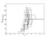 |
Fig. 1 Illustration of the merger tree of HII regions. Each black line represents an ID evolution with the redshift for a distinct HII region. For clarity, we represent here only the ID evolution for 30 regions. |
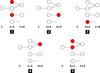 |
Fig. 2 Illustration of the properties that we can follow with the merger tree. In each diagram, red items symbolize the kinds of properties that we follow. 1: The number of new HII regions between two snapshots; 2: the number of growing ionized regions; 3: the number of HII regions that recombine; 4: the number of HII regions resulting from mergers and, 5: the number of parents involved for an HII region resulting from mergers. |
In Fig. 2 we illustrate the typical properties that can be investigated through the merger tree:
-
the number of new HII regions between twosnapshots;
-
the number of growing ionized regions;
-
the number of HII regions which recombine;
-
the number of HII regions resulting from mergers;
-
the number of parents involved for an HII region resulting from mergers.
3. Simulations
3.1. Gas dynamics and post-processed radiative transfer
In this section we aim at describing the cosmological simulations of reionization performed and analyzed with the merger tree methodology. These simulations were part of a set of experiments at several resolutions and fully described in Aubert & Teyssier (2010) and only a brief summary of the methodology will be given here.
The evolution of the gas and sources distribution were provided by outputs of the RAMSES cosmological code (Teyssier 2002) that handles the co-evolution of dark matter, gas and star particles using an adaptive mesh refinement strategy. The hydrodynamical equations are solved thanks to a second order Godunov Scheme with an HLLC Riemann Solver. The gas is assumed to be perfect with a 5/3 polytropic index. Metals are included and taken in account in the cooling of the gas. The star formation is included following the prescription of Rasera & Teyssier (2006) as well as supernovae feedback.
Initial conditions were generated on 10243 grids, according to the WMAP 5 cosmology (Komatsu et al. 2009) using the MPgrafic package and white noise statistics from the Horizon collaboration (Prunet et al. 2008). Two box sizes were considered, 50 and 200 Mpc/h, both with a 10243 coarse grid resolution + 3 levels of refinement and simulations were conducted down to z ~ 5.5. The refinement strategy is quasi-lagrangian with finer levels being triggered when the mass within a cell is 8 times the mass resolution. The large box is less subject to finite-volume variance effects but lacks resolution whereas the 50 Mpc/h box better resolve small scales physics (such as star formation) but is more prone to cosmic variance and its percolation process during reionization may be already affected by periodic boundary conditions
The radiative transfer was included as a post-processing step using the ATON code (Aubert & Teyssier 2008) in all simulations. It tracks the propagation of radiation on a 10243 coarse grid using a moment-based description of the radiative transfer equation. It can reconcile the high resolution and the intensive time-stepping of the calculation thanks to Graphics Processing Units (GPUs) acceleration obtained through NVidia’s CUDA extension to C (see Aubert & Teyssier 2010, for further details of the implementation). ATON also tracks atomic hydrogen processes, such as heating/cooling and photo-ionization, and can handle multiple group of frequencies, even though only a single group of photon has been dealt with in the current work. The typical photon energy is 20.26 eV, corresponding to the average energy of an hydrogen ionizing photon emitted by a 50 000 K black body: such a spectrum is a good approximation of a salpeter IMF integrated over the stellar particles mass assumed here (see e.g. Baek et al. 2009). Calculations were run on 64−128 M2068 NVidia GPUs on the hybrid sections of the Titane and Curie supercomputers hosted by the CCRT/CEA facilities. Having post-processed the simulations, we applied the merger-tree methodology described in the previous section to the ionization fraction field degraded at a 5123 resolution, making them easier to analyze.
3.2. Ionizing source models
At each resolution, three different models were considered for the sources: two considered the self-consistent stellar particles spawned by the cosmological simulation code. The third one uses dark matter halos as proxies for the sources. All the models were tuned by trial and error to provide a complete reionization by z ~ 6.5−5.5 and a half-reionization at z ~ 7. Sources were included in the radiative transfer calculation following the same procedure as in Aubert & Teyssier (2010).
3.2.1. Star models
The star formation recipe is described in Rasera & Teyssier (2006) and assumes that above a given baryon over-density (δ ~ 5 in our case), gas transforms into constant mass stars (1×10⁶ M⊙ and 2×10⁴ M⊙ in 200/50 Mpc/h boxes) with a given efficiency (ϵ = 0.01).
The number of stellar particles found at z ~ 8.5 (which corresponds to the peak of HII regions number as seen hereafter) is 8500 (resp. 35 500) in the 200 Mpc/h (resp. 50 Mpc/h) simulations. Even though it is now standard, the modelization of the formation of stellar particles in cosmological simulations remains a complex and subtle matter. Among other effects, it depends strongly on the resolution: the growth of nonlinearities is scale-dependent, and as a consequence the simulated star formation rate depends on the ability of the simulation to resolve high-density peaks (see e.g. Springel & Hernquist 2003; Rasera & Teyssier 2006, and references therein). Therefore poorly resolved simulations tend to develop a population of stars at later times and at a slower rate than more resolved ones. This limitation is further emphasized during the reionization epoch at large z. As a direct consequence, the amount of ionizing photons is usually underevaluated if taken directly from star particles even though the situation improves as the nonlinearities evolves in the simulations. For instance, with the number of resolution elements and refinement strategy used in the current work, a 12.5 Mpc/h box would be needed to achieve a convergence in the number of emitted photons (Aubert & Teyssier 2010). Otherwise, the star particles may even be too scarce to reionize the cosmological box. Furthermore, these sources are subject to stochasticity and contribute to the UV flux only during the lifetime of strong UV-emitting stars (that we chose to be 20 Myr). As this component fades away in a given stellar particle, the latter may not be replaced by a neighbor. Until a stationary regime of source renewal is installed, these numerical artefacts due to source discretness and lack of convergence may lead to blinking emitters of a numerical nature, and therefore to artificial recombining HII regions unsustained by inner sources, with no relation to actual starburst episodes.
On the other hand, these stellar sources are directly generated from the simulation, are simulated self-consistently with the gas physics, and do not require any additional processing to compute the sources locations and emissivities. One may suggest that a simple correction may be enough to correct from the low-resolution effects. The simplest is to consider that stellar particles sample the location of the main UV sources correctly, and a constant fudge factor would provide the adequate number of ionizing photons to reionize at z ~ 7−6. Such a model is named “SXX” hereafter, where “XX” stands for 200 or 50 depending on the box size. A more sophisticated one requires that not only is the adequate number of photons generated at z = 6 but also at each instant. Since the lack of resolution is more critical at early times, it implies a stronger correction at high z than later on. Aubert & Teyssier (2010) have shown that the correction is exponential with characteristic times depending on the resolution. A drawback of this type of correction is that sources end up as individually decaying with time: if the renewal rate of stellar particles is not high enough, this decay could affect the simulated reionization. In this model, stellar particles have boosted emissivities per baryon at early times and is named “SBXX” hereafter, XX standing for the box size. It should be noted that the density contrast chosen here to trigger star formation can be seen as low and is chosen to allow star formation at our moderate spatial resolution and at redshifts where nonlinearities are weak on our scales. The value chosen here is similar to the one used by, e.g., Nagamine et al. (2000) at the same resolution and is slightly more permissive than most of the thresholds reviewed, e.g., in Kay et al. (2002) with typical values of δ ~ 10. However, even with such criteria, significant factors should be applied to the luminosity of these stellar particles to produce enough photons to obtain standard reionizations histories. As shown hereafter, the ionized patchiness of these models tend to be less structured on small scales than for halo-based models, while nevertheless having their overlap process shows the same overall properties. Overall it indicates that star particles are not overproduced.
In Fig. 3, one can see that the S200 and S50 stellar models show different slopes for the cumulative number of photons. It results from the fact that the same number of photons must be produced from fewer star particles and in a shorter period for the large box. At both resolutions, two ionizing photons per hydrogen atom have been produced when reionization is completed at z ~ 6.5. The SB models are as expected “converged”: as the photon production become stationary, the same number of photons is produced in both box sizes. Compared to the star models emissivities, the boosted ones are greater at early times, then smaller for z < 7.5, to achieve the reionization at the same epoch. On a more general note, one can see that stellar particles appear earlier at high resolution as expected.
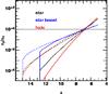 |
Fig. 3 Redshift evolution of the cumulative number of ionizing photons emitted by the sources relative to the number of hydrogen atoms. The horizontal line stand for one photon per atom. Solid (resp. dashed) lines stand for the 200 (resp. 50) Mpc/h simulations. Black, blue, and red curve stand respectively for the star, Boosted Star and Halo models of ionizing sources. |
Quantitatively, we followed the simple modelization of Baek et al. (2009) to assign an emissivity of 90 000 photons per stellar baryon over the lifetime of a source. For S50 and S200 the enhancement factors to account for convergence issue are 3.8 and 30, respectively, while the boost temporal evolution of the SB50 and SB200 is equal to max(1,aexp(k/t)) with (a,k [Myr] ) = (1.2, 1500) for SB50 and (1.2, 3000.) for SB200, where t is the cosmic time.
3.2.2. Halo sources
As a second choice we adopt a semi-analytical model for the production of ionizing sources based on dark matter halos. Each halo is assumed as a star formation site with an emissivity proportional to the halo mass. This procedure is largely inspired by the work of Iliev et al. (2006b) where a constant mass-to-light ratio is assumed such as the ionizing flux of each halo has the following expression:  (1)where α is the emissivity coefficient. Here we have chosen values of α = 5.9×1043 and α = 3.5×1042 photons/s/M⊙ for both 200 and 50 Mpc/h boxes, respectively. These values were chosen in order to reach a reionization at z ~ 6.5−6 similar to the star and boosted star models. Halos were detected using the parallel FOF finder of Courtin et al. (2011), with a linking length of b = 0.2 and a minimal mass of ten particles. This minimal mass corresponds to 9.8×10⁷ M⊙ for the 50 Mpc/h box and 6.3×10⁹ M⊙ for the 200 Mpc/h box, implying that all halos can be considered as emitters. The number of halos found at z ~ 8.5 is 33 100 (resp. 285 000) in the 200 Mpc/h (resp. 50 Mpc/h) simulations. It should also be emphasized that, unlike star and boosted star models, a whole spectrum of mass, hence emissivities, is available for halos. No lifetime has been assigned to these sources, and a halo would produce photons as soon as it is detected until it disappears or merge. In the following sections we refer to this semi-analytical star formation simulations with the following acronyms: “H200” or “H50” for both box sizes of 200 and 50 Mpc/h.
In Fig. 3, one can see that H50 follows closely S50, implying that with the appropriate correction, stars can mimic halo emission history. A greater difference can be seen in the 200 Mpc/h box, where the H200 model shows a greater slope than the S200 model: there is a greater difference in the buildup of halos compared to the star population at lower resolution, due mostly to the difficulty of achieving star formation density thresholds in large-scale simulations. At z ~ 6.5, roughly two photons per hydrogen atom were produced in all cases.
4. General features
4.1. Ionization fraction
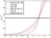 |
Fig. 4 Evolution of the volume-weighted average ionization fraction with redshift for the six simulations. |
Figure 4 shows the evolution of the volume-weighted average ionization fraction as a function of redshift for the three models and for both 200 and 50 Mpc/h boxes. Average ionization curves show a similar value of ⟨ x ⟩ ~ 0.5 at a redshift of z ~ 7. At first glance we see that every model is comparable in terms of ionization fraction. The boosted star model just shows an earlier rising in the ionization curve than in the two other models for both box sizes. Conversely in the star and halo models the ionization curves rises later (z ~ 10−9) but the reionization is achieved earlier than in the boosted star model. These differences are attenuated in the 50 Mpc/h box where the ionization histories approach each other.
4.2. Optical depth
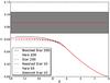 |
Fig. 5 Evolution of the Thomson optical depth with redshift for the six simulations. |
Figure 5 shows the evolution of the optical depth as a function of redshift for the six simulations given by
 (2)
(2)
where σt is the Thompson cross section of the electron, and ne(z) = ⟨ x(z) ⟩ nH(z) the density of electrons released by ionized hydrogen atoms at redshift z. We also represent the constraint range obtained from the five-year release of CMB measurement made by the WMAP collaboration (Komatsu et al. 2009) at the 1σ level.
We immediately see that all the simulations converge in terms of optical depth. The 200 Mpc/h box simulations reach the same value at z ~ 8. The only difference is that the optical depth is slightly greater in the boosted star model before z ~ 8. This is naturally explained by the fact that the ionization history is more extended in this model as seen with the ionization curve in Fig. 4. In the 50 Mpc/h box, the curves become almost superimposed from z ~ 10. Again, this confirms that all the simulations are comparable.
4.3. Ionization fields
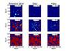 |
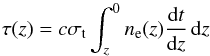
Fig. 6 Ionization map for the three ionizing sources models for three distinct redshift for the 200 Mpc/h size box. The colors encode the different identification number allocated to the HII regions by the FOF algorithm. |
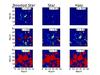 |
Fig. 7 Ionization map for the three ionizing sources models for three distinct redshifts for the 50 Mpc/h size box. The colors encode the different identification number allocated to the HII regions by the FOF algorithm. |
The maps of Figs. 6 and 7 show the ionization field maps for the three models for both 200 and 50 Mpc/h boxes. In each figure, the color encodes an individual HII region detected by the FOF procedure.
At z ~ 10.5 and z ~ 8.4, the basic features of the three types of reionization can be spotted: SB models exhibit a few regions with large radii, whereas H models have smaller and numerous individual regions. The S models are intermediate with larger ionized patches than detected in the halo-based simulations but more individual regions than found in the SB models. As such, it reflects the differences in source modeling where halos are more numerous than stellar particles, so they share ionizing photons over a larger number of weaker sources. On the other hand, SB models produce large regions at the earliest redshifts because of the strong initial correction to the source emissivity, and this favors large regions and potentially early overlaps.
At the end of the reionization at z ~ 6.9 and in all models, a single large HII region is detected by the FOF method and results from a connected network of multiple ionized regions. Nonetheless, the halo model presents a greater resilience to percolation since it presents a map more structured with more individual HII regions.
When the spatial resolution is increased with the 50 Mpc/h box, Fig. 7 shows the same tendencies as in the 200 Mpc/h box. The H50 map presents the most regions with the smallest sizes until late phases of the reionization, and the SB50 still presents the fewest regions with the largest sizes. S50 still represents an intermediate case. Overall and as expected by the greater spatial resolution, the ability to capture the clustering and more sources in a 50 Mpc/h box, these maps present a higher level of granularity and more individual regions than the 200 Mpc/h versions.
5. Merger-tree properties
Our main interest is to investigate the impact of the ionizing source models on the reionization history. Typically, we see what quantities are retained from one model to the next and how these models create differences in the observed history.
5.1. Evolution of the number density of HII regions
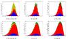 |
Fig. 8 Evolution of the number density of each kind of HII region as a function of redshift for the three models of ionizing sources and for both boxes of 200 and 50 Mpc/h. Panels a)–c) respectively represent the distribution for the Boosted Star, the Star, and the Halo models for the 200 Mpc/h box, while the panels d)–f) are for the same models but for the 50 Mpc/h box. The colors stand for the new HII regions (blue), the expanding regions (red), the regions that will recombine (yellow), and the regions resulting from mergers (green). |
Figure 8 shows the evolution of the number density of ionized regions as a function of redshift for the three models of ionizing sources and for both box sizes. We also distinguish the number of each type of HII regions: new regions, those resulting from mergers, those expanding without merging, and those recombining. We note that the distributions present the same general shape regardless of the source model. They all show their maximum number of regions at broadly the same redshift, zpeak, for both spatial resolution at z ~ 8 and z ~ 9 for 200 Mpc/h and 50 Mpc/h, respectively. Before zpeak, HII regions appear and expand, populating the box with more and more regions. We can refer to this period as the “pre-overlap” period where the reionization is dominated by the expansion and the birth of new HII regions. Conversely, after zpeak, HII regions begin to merge intensively and decrease in number during an “overlap period”, that continues until the reionization is completed. Even though the shape of the distributions is similar, the absolute number of HII regions is much greater in the halo model than in the two stellar ones and with a greater discrepancy in the 50 Mpc/h box. This absolute number remains within the same order of magnitude between the star and the boosted star model for both boxes. This difference is not surprising and typically reflects the difference in the relative number of ionizing sources produced from one model to the next. Indeed, the number of dark matter halos assumed as ionizing sources in the semi-analytical model is greater than the number of autoconsistent ionizing sources generated in both star models: at z = 8.5 there are about four (resp. eight) times more halos than stellar particles in the 200 Mpc/h (resp. 50 Mpc/h), and it corresponds to the factor measured in terms of detected HII regions. Finally, when splitting these distributions into different types of ionized regions (new, expanding, merging, and recombining), they follow the overall pattern of increase and decline after zpeak with differences explained in the next Sect. 5.2. We only mention the case of new regions that also follow the same pattern, even though at face value mergers only affect pre-existing ionized patches. It should be recalled that, as reionization progresses, the amount of neutral volume decreases, limiting the possibility of having new sources in a neutral area. As a result, new regions are also affected by the overlapping process, albeit indirectly.
5.2. Number and volume fraction of the different types of HII regions
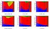 |
Fig. 9 Evolution of the proportion of each kind of HII regions as a function of redshift for the three models of ionizing sources and for both boxes of 200 and 50 Mpc/h. Panels a)–c) respectively represents the distribution for the Boosted Star, the Star, and the Halo model for the 200 Mpc/h box, while the panels d)–f) are for the same models but for the 50 Mpc/h box. The colors stand for the new HII regions (blue), the expanding regions (red), the regions that will recombine (yellow), and the regions resulting from mergers (green). The black vertical line shows the peak of the absolute number of HII regions: zpeak. |
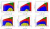 |
Fig. 10 Evolution of the volume fraction of each kind of HII regions as a function of redshift for the three models of ionizing sources and for both boxes of 200 and 50 Mpc/h. Panels a)–c) respectively represents the distribution for the Boosted Star, the Star, and the Halo model for the 200 Mpc/h box, while the panels d)–f) are for the same models but for the 50 Mpc/h box. The colors stand for the new HII regions (blue), the expanding regions (red), the regions that will recombine (yellow), and the regions resulting from mergers (green). The black vertical line shows the peak of the absolute number of HII regions: zpeak and the black horizontal line shows the volume fraction of one cell of the grid. |
To emphasize differences in the histories of the various kind of regions, Fig. 9 shows the evolution of their relative proportion (rather than their number density) in terms of number and Fig. 10 presents the volume fraction of the whole simulated boxes occupied by each type of HII region.
5.2.1. Recombining regions
The most striking feature of SB models (and to a lesser extent S models) is the presence of recombining HII regions, tracked as connectionless branches in the merger tree. Recombination can be driven by one of two main factors: high-density features or evolving sources. The evolution of the density is common to all experiments and the lack of such regions in H models indicates that it is unlikely to be the main origin of these peculiar regions. Nevertheless, a hint of this “density” effect can be seen in the larger number of such regions in the S50 model compared to S200 or in their marginal presence in H50: higher resolution leads to higher contrasts, hence higher recombination rates. On the other hand, stellar sources are more prone to variation than halo sources. First, they exhibit some level of stochasticity, so that sources that turn off may not be replaced through an efficient renewal process in order to sustain some regions, whereas “halo” sources have a continuous emission. It explains the lack of such regions in H models and their detection in S and SB models. Second, SB models have sources with decreasing individual emissivity, leading to a typical scenario where strong early sources produce large regions that see their inner ionizing engine becoming progressively weaker or stars being replaced by weaker ones, eventually leading to recombinations. Combined with stochasticity, this effect can lead to regions that are being dissolved, potentially at several places within one region. Increasing the resolution tends to diminish the contribution of this type of regions in SB50 models: the differential boost applied to source is weaker than in SB200, hence decreasing the effect of inner exhausted engine and the stellar renewal is more efficient, leading to a production of ionized regions closer to a stationary regime. Looking at Fig. 10, it is interesting to note that in all the cases where they are detected, recombining regions stand for a small fraction of the total ionized volume: between ~ 10-7 for the H50 model and ~ 10-5 of the total volume of the box for the SB200 model. Therefore, even if recombining regions are good indicators of the behavior of the source models, it can be seen that they only correspond to an almost negligible fraction in terms of volume and can to some extent be considered as marginal.
5.2.2. Regions in expansion
Expanding regions are detected as having only one “parent” and expand without additional event. In absolute numbers (see Fig. 8), their number peaks at zpeak, and their proportion is always dominant until the very end of the reionization. Incidentally, it shows that the temporal sampling is high enough to generally track the initial expansion of individual regions. Also, that such regions are still detected in the later stages suggests that even in the later stages of the percolation, not all the regions are involved in a general merging process: some regions still have room to experience stages of quiet growth before eventually becoming part of the global ionized background. In terms of volume (see Fig. 10), expanding regions are the main contributors to the total ionized volume in every model until typically zpeak. This is not surprising since the expanding regions are naturally much larger than the new regions and are always dominant in number (see Fig. 8). Once the overlap starts to be efficient, merged HII regions supersede the expanding ones in volume, as expected.
5.2.3. New regions
New regions (without parents in the tree) track the formation of new sites of emission, i.e. star or halos forming in distant enough areas of pre-existing ionized volumes. Of course, any source that appears within an ionized region because of clustering will not contribute to this population. Their proportion (and their absolute number) present regular spikes. The tree is constructed using a time sampling that is different than the sampling used to include sources in the radiative transfer calculation. The tree sampling frequency is low enough that at least a new generation of source has been included between two snapshots and new regions are thus detected. But this frequency is also low enough that two generations of new sources were, regularly, included in the RT calculation between two snapshots, creating bursts of new regions. The presence of these spikes does not affect our analysis and conclusions.
All experiments usually show an initial gradual decrease in the proportion of new regions. In the 50 Mpc/h experiments, this decline stays until the end of the reionization. It is related to a pile-up effect of pre-existing HII regions: until zpeak their numbers increase at a higher rate than for new regions. For instance, regions keep growing without efficient merging over several generations of new HII regions: it increases the number of pre-existing regions and mechanically decreases the proportion of the new ones at any given moment. After zpeak, the proportion of new regions increases in 200 Mpc/h experiments and arguably remains constant in 50 Mpc/h ones.
By construction, the overall number of ionized sites decreases in this “post-overlap” period, indicating that among these sites, new regions suffer to a lesser extent of the percolation process. While the destruction rate of pre-existing HII regions is important, new stars or halos thus manage to appear in neutral areas, sustaining (in the 50 Mpc/h box) or even increasing (in the 200 Mpc/h box) the relative contribution of the new regions.
This increase in the contribution of new regions seen in S200 and H200 indicates that the destruction of pre-existing regions is more sudden than at higher resolution: it was suggested in Fig. 8 where the post zpeak evolution is smoother at high resolution or in Fig. 4 where the average ionized fraction exhibits a sharper evolution at reionization. Regarding this sharper evolution, we emphasize that a more accurate tuning of the source emissivity could have increased the matching of the reionization history of the H and S models and may be the origin of this difference between high and low resolution. It may also be the result of different behavior in the propagation of fronts at low resolution (with faster fronts and weaker shielding), leading to a more radical percolation in the 200 Mpc/h simulations than in the 50 Mpc/h boxes. Finally, we mention that the presence of a strong recombining component in the SB200 model leads to a totally different evolution of the new regions’ contributions that remain broadly constant at all redshifts with a weak dip at z ~ 10. Without these recombining regions, a rising relative weight of new regions would also be exhibited, albeit starting much earlier than zpeak.
Regarding their volume fraction (see Fig. 10), these newly detected regions only represent a maximum of ~ 10-4−10-3 of the total volume even if there is a sizable number of this kind of region detected. This is understandable because of their very nature: new regions are by definition expected to be small, since they have just appeared, and their number cannot compensate for this. Interestingly, the total volume occupied by the new regions remains broadly constant until overlap, indicating that, even though sources increase in number with time(and thus the potential number of new regions), it competes with the gradual decrease in available neutral volume. These two effects “conspire” to keep constant the volume imprint of the new patches on the network of HII regions.
5.2.4. Regions resulting from mergers
These regions have more than one parent and therefore result from the merger of several regions. They track the coalescence of pre-existing regions into larger ones and eventually track the final overlap into a single large HII region at the end of reionization. This last stage can be seen in all models where a late snapshot exists where 100% of the detected region results from mergers, an indication of the ultimate merger. The S and H models present similar evolutions for the merger populations. Their proportion is coincidentally maximum at zpeak: as the number of ionized patches gets larger, a greater fraction of them are involved in mergers, indicating a crowding or clustering effect where a smaller volume is available for expansion as the number of HII regions increase. Later on, for z < zpeak, the proportion of mergers decreases, indicating that only a subset of the ionized regions actually do merge, potentially only one that would phagocyte the others, reducing the overall number of individual regions until the end. The peak of mergers fraction could therefore be seen as the rise of one or several dominant regions, and this rise appears when the number of individual region is at a maximum.
Comparing the two resolutions, it can be noted that mergers are concentrated over a narrower range of redshifts at low resolution, whereas merger can be detected at a significant level during the whole experiment in the S50, H50 and SB50 models. First, it can be the consequence of the slightly more extended history of reionization in 50 Mpc/h simulations, already mentioned regarding the ⟨ x(z) ⟩ trends (see Fig. 4). Second, sources and individual regions are more numerous at any time and in a smaller volume, favoring a more generalized contribution of mergers over a wide range of redshifts.
Finally, it should be noted that the SB200 model presents an early peak in the fraction of merger, at z ~ 10 instead of z ~ 8 for all the other experiments, with an almost zero contribution later on, even though the absolute number of regions manages to decrease at some point. It suggests that the onset of the percolation started earlier, owing to early, large HII regions induced by the large initial boost of this model, and this created a single region that monopolizes the merger process. Interestingly, in this case zpeak occurs later, indicating that, while this main region grows, a significant amount of neutral volume remains to host the apparition of new regions.
Finally, Fig. 10 clearly indicates that these merger regions dominate the ionized volume at z ≤ zpeak. This was not obvious given that their number density is always the lowest contribution (cf. Fig. 8). It is indicative that few of these regions produce a network that dominates the ionized volume and/or that such regions are individually very large, as one would expect from their being the result of several mergers. This point is assessed in greater detail in the next sections.
5.3. Sizes of HII regions
5.3.1. Sizes distribution with redshift
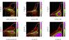 |
Fig. 11 Evolution of the HII regions radius distribution as a function of redshift for the three models of ionizing sources formation and for both boxes of 200 and 50 Mpc/h. Panels a)–c) respectively represents the distribution for the Boosted Star, the Star and the Halo model for the 200 Mpc/h box, while the panels d)–f) are for the same models but for the 50 Mpc/h box. The brightest red cells represent the location in the distribution populated by a single HII region, other red tones up to the brightest green cells span distribution densities from a couple of HII regions up to a value corresponding to half the maximum value of the distribution. Finally, the purple tones (from the darkest to the brightest) denote the maximum values. The evolution of the average radius and the evolution of the radius of the main region are shown by the solid and dashed white lines, respectively. |
Figure 11 shows the evolution in the distribution of the HII regions radii at each instant as a function of redshift for the 200 and 50 Mpc/h boxes. Like Friedrich et al. (2011), we computed the volume of the HII region and then derived the effective radius corresponding to a sphere of equal volume through the following expression R = [3/(4π)V] 1/3. We also represent the radius evolution of the last HII region which remains at the end of the simulation. With the help of the merger tree we follow this region back in time and calculate the radius of its main progenitor at each instant. In addition we also show the evolution of the average radius of HII regions as a function of redshift.
Typically, each distribution seems to trace the underlying ionizing source prescriptions related to the model considered. The S models have a constant star emissivity with redshift. This is reflected in the radii distributions where ionized regions are concentrated with a constant radius about r ~ 4 Mpc/h over the whole range of redshift in the 200 Mpc/h box. We find a gap at about r ~ 2 Mpc/h in the size distribution where there are only a few regions with radii under this constant radius. This would indicate that the time sampling used here cannot entirely capture the fast tracks followed by the HII regions in the radius-redshift space with strong inner sources. This effect is attenuated for the 50 Mpc/h box (that contains typically weaker sources and HII regions with lower growth rates) where we observe a more continuous distribution even if a typical cutoff radius of r ~ 0.4 Mpc/h remains, with smaller occupation numbers at low values.
On the other hand, the halo model implies that each of them has an emissivity proportional to its mass. As these masses cover a wide range, we find a wide range of radii for the resulting HII regions in the distribution of the 200 Mpc/h box. The regions are concentrated in larger intervals of radii than in the other models that typically trace the underlying mass range of halos. The shape of the distribution is almost the same when we consider the 50 Mpc/h experiment, with smaller regions since smaller halos are available at higher resolution.
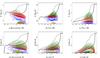 |
Fig. 12 Evolution of the radius distribution of each kind of HII regions as a function of redshift for the three models of ionizing source formation and for both boxes of 200 and 50 Mpc/h. Panels a)–c) respectively represents the distribution for the Boosted Star, the Star, and the Halo model for the 200 Mpc/h box, while the panels d)–f) are for the same models but for the 50 Mpc/h box. The colors stand for the new HII regions (blue), the expanding regions (red), the regions that will recombine (yellow), and the regions resulting from mergers (green). In addition the solid and dashed black lines represent the radius evolution of the main region end the evolution of the average radius for the HII regions, respectively. |
Finally, the SB models have a boost for the star emissivity that decreases with redshift. Indeed the distributions show, at early times, large HII regions detected without small counterparts. This gap would be the result of the very powerful boost for ionizing sources at high redshift combined with the time sampling of the simulation, which allows only regions to be detected when they have a large radii early in the reionization. Then we can observe a decreasing gradient for the typical radius of the regions as the boost for the emissivity decreases with time. Surprisingly we find a bimodal distribution from a redshift of z ~ 9 until the reionization at z ~ 6. Some HII regions are concentrated with radii below or under ~ 1 Mpc/h with a gap in the distribution for this value. To a lesser extent, the same effect could be seen in the S200 model. Those regions with radii under ~ 1 Mpc/h could be the recombining regions that we have found in Fig. 9. This could also be combined with the fact that around these redshifts the boost emissivity falls below a given value. Then, the time sampling of the simulation would become fine enough to detect some new or expanding regions with these radii. We further investigate this in the Sect. 5.3.2. For the SB50 model, this bimodal distribution disappears: a weaker boost amplitude and variation combined to a more stationary production of stars promotes better tracking of regions’ sizes as they grow and reduce the contribution of recombination, as seen earlier.
Considering the S and H models again for both box sizes, it is interesting to note that the S model produces a truncated version of the H one. Above the cutoff radius (0.4 Mpc/h (resp. 4 Mpc/h) in the S50 (resp. S200)), the S and H distributions are quite similar. At smaller radii, S has fewer objects than H. It is indicative that there is a scale above which the clustering of halos combined to their own mass-proportional emissivities produce a similar radii distribution to the one provided by the clustering of stellar sources and their own constant emissivity. On smaller scales, the stellar sources are too scarce to reproduce the regions created by halos, resulting in overpowered individual sources with large radii. On larger scales the two approach produce equivalent size distributions and with an appropriate calibration, hydrodynamically created sources can match the halo result. It should be noted that this typical scale appears at lower values in S50 models because sources are more numerous and less prone to stochasticity, and therefore they converge toward the halo model behavior on smaller volumes.
Finally, all the experiments present a single main HII region that dominates in size. It appears at z ~ 8 in the S200 and H200 models and much earlier (z ~ 9) in the SB200. As suggested by the previous study of merger populations, this is likely the consequence of the boost that creates early large regions that merge at high z to give the dominant one. Interestingly, the dominant region of the late reionization is not dominant in size at every redshift. This is indeed the case for the H200 model and to some extent for the S50 model too, but in all the other case this region started as a non special one inside the population, at least from the radius point of view. Furthermore, the first progenitor of the dominant region is among the very first ionized regions of the H200 and H50 models, but it appears later in the S and SB experiments. It is noteworthy that, even though we argued that S and H model produce similar populations (for larger regions than the cutoff radius), it seems that differences can persist for individual cases, especially for the buildup of the dominant region. As we see in the next sections, the channel through which this specific region grows (through expansion rather than merger) also differs as hinted at by the difference between the smooth evolution of the dominant region of H models and the sharp, kinked, and late rise of its equivalent in, e.g., the S200 model.
5.3.2. Radius distribution of the different kind of HII regions
Figure 12 presents the size distribution for each kind of HII regions as a function of redshift for all three models and for both 200 and 50 Mpc/h boxes. Here we show the same distribution as seen in Fig. 11 but by plotting the contours related to each type of HII region that we can discern. Once again we show the evolution of the average radius of the region and the evolution of the radius of the last HII region as in Fig. 11.
Initially, we observe that each kind of HII region occupies a dedicated range of radii in the whole distribution for all models and for both 200 and 50 Mpc/h box sizes. As expected, new regions occupy the narrow range of radii, while the regions resulting from mergers are those that populate the top of the distribution. The expanding HII regions are in the middle with radii larger than the new ones and smaller than those that will merge. We can also see in each model that the peak of the distribution of Fig. 11 corresponds to a radius range that is simultaneously covered by the three kinds of HII regions. Alternatively, we could have imagined a clear separation between the different range of radii covered by the different kinds of HII regions instead of the observed overlap of the different distributions. This tells us first that the time sampling here allows us to detect HII regions with same radii but belonging to different kinds of HII regions with different paths in the radius-redshift space. It also indicates that the peak of the radii distribution must be understood as the most likely radii of detection, with a mix of HII regions at different stages in their evolution (newborn, growing, or merging).
Interestingly, for each kind of region, we find the properties of the underlying ionizing source models in the evolution of the radius distribution with redshift. In other words, the R(z) distribution for the size evolution of each kind of regions as function of redshift is dictated by the R(z) distribution of the new regions and is propagated to the other kinds of regions. We thus can see a similar R-z relationship for the expanding region and those resulting from merger with a simple translation. In the star models S50 and S200, the new regions appear with a relatively constant range of radii during the whole reionization; again, it reflects the typical constant emissivity of the stars appearing during the whole simulation, combined with the time sampling used here. The expanding regions and those resulting from mergers also show this constant radius range but translated to greater radius ranges. The S50 allows to track smaller new regions thanks to its higher resolution in terms of sources with smaller individual emissivity: as a consequence, all subsequent types show smaller typical radii than in the S200 model.
The H200 model presents new regions that appear with more distributed sizes than in the S50/S200 models and that typically result from the mass range of the dark matter halos that are assumed as ionizing sources. Then the expanding regions cover a much greater radius range than in the two other models, and we find the same trend for the regions resulting from mergers. The last point indicates that the merger process is not dominated by a few large regions as in the two other models but that is also involves sets of small HII regions. In the H50 model the mixing is more pronounced, and the ranges of radii covered by each kind of regions overlap. Highly clustered regions are more represented at high resolution where dense sets of small halos with small regions can also merge. In H200, mergers occur at later stages in radii evolution, in a more homogeneous distribution of halos at low resolution.
Finally, SB200 shows that new regions appear with decreasing radii as reionization progresses and as the boost for the star emissivity decreases. The expanding regions and those resulting from merger show the same R-z decreasing trend, triggered by the new regions population properties. It should be noted that at some point (z < 9), new regions can be detected at small radii: the declining boost leads to individual regions that appear with smaller size and lower growth rate, increasing the likelihood of spotting them at small radii. A weaker R-z slope is found in the SB50, as a consequence of a smaller boost correction at higher resolution. As expected, new regions with small radii are found earlier (for z < 12) and usually share a greater number of broad features (like the range of radii for each type) with the S50 model.
We finally focus on the HII regions that recombine in the size distributions of each model. As expected in Sect. 5.3.1, we find that regions that will recombine are those with radii below the radius of ~ 1 Mpc/h in both SB and S models and at both resolutions. As already mentioned, the recombination is driven either by density or by a modification of the sources. In the case of SB models, it is fairly obvious that strong early sources create large HII regions that may be unsustainable by later generations of sources, which are individually weakened by construction of the boost. Furthermore, the boost guarantees a general convergence, but locally a strong early source can be replaced by too few weaker, later sources, especially if the source renewal is subject to stochasticity. Once sources become too dim, it leads to the fragmentation of regions and recombinations on small scales. S models also present some degree of recombination, even though they do not contain declining sources. These recombinations can be explained by local dense patches, and this could be supported by such regions only appearing at later times (z < 9) in the S200 model, when local clustering is high enough. Furthermore, in both S50 and SB50 models, these regions can be found over extended periods compared to their 200 Mpc/h equivalent, related to the higher likelihood that dense patches that trigger recombination are found at high resolution.
5.4. Mergers of HII regions
5.4.1. General evolution of the merger process of HII regions
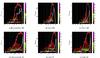 |
Fig. 13 Distribution of the number of parents for the HII regions resulting from merger as a function of redshift for the three kinds of ionizing sources and for both box sizes of 200 and 50 Mpc/h. Panels a)–c) respectively represent the distribution for the Boosted Star, the Star, and the Halo model for the 200 Mpc/h box, while the panels d)–f) are for the same models but for the 50 Mpc/h box. The brightest red cells represent the location in the distribution populated by a single HII region; other red tones up to the brightest green cells span distribution densities from a couple HII regions up to a value corresponding to half the maximum value of the distribution. The purple tones (from the darkest to the brightest) denote the maximum values, and the evolution of the average number of parents and the evolution of the number of parents of the main region are represented with the solid and dashed white lines, respectively. |
Figure 13 is restricted to regions that have more than one parent, i.e. that result from mergers. It presents the redshift evolution of the distribution of the number of parents. It can be seen as a measure of the patchiness or granularity of the overlapping process and is also a first indication of the inner complexity of the regions: an ionized volume that results from tens of progenitors is shaped (like e.g. the front propagation, its growth rate, or the inner distribution of UV flux) by the different properties of at least tens of sources, whereas an HII region coming from a binary merger is likely to be, maybe naively, more straightforward to relate to its inner sources. In addition, we show the evolution of the average number of parents and the evolution of the number of parents for the last remaining region at the end of the simulation. Again, with the help of the merger tree we follow this region back in time and evaluate its number of parents at each instant. The color code in the distributions is identical to the one used in the Fig. 11.
First, in most of the models the mergers between regions operates in a binary-tertiary manner as seen with the peak at ~ 2−3 in the distributions. It is essentially an indication that the temporal sampling of the tree is fine enough to track individual mergers, whereas a coarser grained sampling would have typically presented a higher value. One exception is the H50 model, where such mergers are clearly missing from z ~ 10 to z ~ 7. In this case, the abundance of clustered individual regions at high density is much greater than in other models and leads to multiple mergers during a single time step for a given region.
Second, in each model we find the emergence of a single region, which is the result of more mergers than the other regions. In the S200 and H200 models, this region appears at z ~ 8 and earlier in the SB200 one, at z ~ 9. The same discrepancy can be found at higher resolution with a formation at z ~ 9 for the S50 and H50 models and z ~ 10 in the SB50. Interestingly, these merger-dominant regions appear at the same moment as the radius-dominant region discussed in the previous section. In Fig. 13, the evolution of the number of parents of the radius-dominant region unsurprisingly matches the path of the merger-dominant one. Thus, a moment exists when an HII region begins to monopolize the merger process in the box. Then the region grows faster by successive mergers and will quickly dominate other regions in size. From this instant (called zBKG), the probability that a location is part of the general UV background, instead of being irradiated by a local source, increases and can be considered as the onset of the overlapping process. This is typically the moment when, on average, the “local” information about the reionization process starts to be lost to the benefit of a single reionization history.
Size is an important factor for regions to get high numbers of progenitors, since a larger volume naturally promotes encounters with distant ionized patches. However, it can be noted that the radius-dominant region is only one among the merger-dominant regions. Clearly the distribution shows regions with more progenitors, and this is especially the case for H200 and H50 models: the high density of sources and their clustering can induce a high merger rate in smaller volumes. More generally, high-resolution experiments present a greater merger rate thanks to a higher number of sources and higher local clustering. Also H models can achieve a number of progenitors that are tenfold greater than the S and SB equivalent as another consequence of large number of halos. The two stellar models also differ in the number of regions with a large number of progenitors: close to zBKG, S models present clear detection of regions with a number of progenitors close to those found for the radius-dominant one (10−50 progenitors), whereas in SB models such regions are seldom found. It indicates that the early buildup of a dominant region in the SB model tends to prevent the formation of separate regions that aggregate several sources on their side, probably because they were incorporated early in this dominant volume. At higher resolution the discrepancy is weaker, but in the S50 models, the dominant region shares the property of having a large (>10) number of progenitors with other regions.
5.4.2. Growth of the main HII region
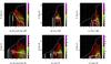 |
Fig. 14 Distribution of the HII regions sizes for the regions that merge with the dominant region as a function of redshift for the three kinds of ionizing sources and for both box sizes of 200 and 50 Mpc/h. Panels a)–c) respectively represent the distribution for the Boosted Star, the Star, and the Halo model for the 200 Mpc/h box, while the panels d)–f) are for the same models but for the 50 Mpc/h box. The brightest red cells represent the location in the distribution populated by a single HII region; other red tones up to the brightest green cells span distribution densities from a couple HII regions up to a value corresponding to half the maximum value of the distribution. The purple tones (from the darkest to the brightest) denote the maximum values. The evolution of the average radius for the regions that merge with the dominant region and the evolution of the radius of the main region are represented with the solid and dashed white lines, respectively. |
In this section we aim at understanding how the dominant region leads to a loss of information about the expansion process of other regions. By looking at the evolution of the properties of the regions that merge with the dominant one, we evaluate how each model is resistant to the emergence of this main HII region.
Figure 14 presents the evolution of the radius distribution for HII regions that merge with the radius-dominant one for all models and both 200 and 50 Mpc/h boxes. The color coding of the distributions is identical to the one used in Figs. 11 and 13.
Immediately we see that, from a certain redshift, every model presents a radius distribution that is representative of the whole distribution of all HII regions, as discussed previously and shown in Fig. 11. In other words, from a certain moment onwards, the major part of the present HII regions are regions that will merge with the main region in the next snapshot. Thus this moment can be seen as the time when the main region imposes its domination. Then the later this moment appears, the longer the individual expansion process of ionized region can be tracked. In all models and at both resolutions, this moment is broadly coincident with zBKG: from this redshift any region (in terms of size) can be incorporated into the background.
It is also noteworthy to see how this main region is built before it begins to impose its domination. For instance, the earliest stage of the buildup in both H50 and H200 models, does not include any merger and the growth is purely driven by the inner source until z = 9.5 (resp. 11.8) for the H200 (resp. H50) model. The equivalent region in the S200 model is detected later, with a large radius (~3 Mpc/h instead of 0.5 Mpc/h for H200) and immediately incorporates other regions with similar sizes. At higher resolution, the radius-dominant region of S50 is always larger than its H50 counterpart and also incorporates other relatively similar region quite early (at z ~ 14 for instance). Clearly the stronger emissivity of individual stellar sources produces larger progenitors for the S models than for the halo-based ones, promoting a merger-driven growth sooner. Meanwhile, the SB models exhibits the expected and quite different evolutions for the dominant region: the large emissivity correction at early times creates a large dominant region at the earliest stages, and it quickly incorporates other regions also expanded by the boost, hence belonging to the same class of large radius. In particular, SB50 present a whole succession of large regions, close to the white evolution track of the dominant one. For the latter, it implies that its radius is always larger than found in the S50 and H50 models and is driven by mergers much sooner. Previously, we found that high resolution tends to diminish the discrepancies of the SB model, but in the current case, the higher level of clustering in the 50 Mpc/h box leads to a buildup scenario of the main region that is arguably even more distinguishable than H and S models.
6. Summary and conclusion
We developed a new methodology based on the merger trees of HII regions to study the history of reionizations in cosmological simulations with full radiative transfer post-processed by the GPU-driven code ATON on RAMSES hydrodynamical snapshots. We systematically applied the technique in two sets of 200 Mpc/h and 50 Mpc/h simulations, where each set involved three kinds of source model:
-
A halo model where halos act as sources of photons with anemissivity proportional to their mass.
-
A stellar model where star particles produced by the cosmological code act as the sources, with an emissivity corrected to complete the reionization at the same redshift as the halo model.
-
A boosted stellar model, where the same star particles are used but with time-dependent and decreasing correction on the emissivity to reproduce the converged emission of UV photons at each instant.
Corrections are necessary because the self-consistent production of star particles by the hydrodynamical code is resolution-dependent and not fully converged at these resolutions. The emissivities were tuned to produce a similar ionization fraction evolution at both resolutions. HII regions were detected thanks to an FOF algorithm and linked throughout time within a merger-tree structure.
First, the three models present an evolution that is comparable in terms of global features. Indeed, the evolution of the optical depth and ionized fraction present similar shapes in all experiments. The evolution of the number of present HII region reaches a maximum at the same similar redshift for all models and for both box sizes (z = 8.5 and z = 9 for the 200 and 50 Mpc/h experiments). However, the study of the separate evolution of the different kinds of HII regions shows that the intense episodes of mergers occur earlier in the boosted star model, while it occurs later and at the same moment in the S200 and H200 models. Also the SB200 model is sensitive to recombination, owing to sources that are unable to sustain the existing HII regions, while only few recombinations occur in the S200 model and none in the H200 model in the 200 Mpc/h. In the 50 Mpc/h simulations, episodes of mergers are similarly distributed in the three models, whereas increased densities are likely to produce the larger population of recombining patches in the SB50 and S50 experiments.
Second, we investigated the evolution with redshift of the size distribution of HII regions. All models present the emergence of a main region in size from a certain redshift onwards. We also have found that the evolution of the radii distribution is typically related to the evolution of the ionizing source emissivities in each model: a large dispersion of possible radii with small structures in the halo-based models, a similar distribution for the stellar model with a lack of small regions due to stronger and sparser emitters and a distribution strongly skewed toward large regions at early times in the boosted stellar experiments. The discrepancies decrease at higher resolution but remain, especially for the last model. We have then be able to show that this radius-redshift correlation, imprinted in the distribution of new regions is somehow memorized and kept in the distribution of growing and merging ionized patches.
The evolution of the number of parents involved in the percolation of HII regions has also been studied. In all experiments, merger-dominant (with 10 or more progenitors) regions exist and among them one corresponds to the radius-dominant one and drives the reionization. Its domination is delayed in both halo and star model compared to the boosted one. As an illustration, we investigated the size distribution of HII regions assimilated by the main one and found that indeed it becomes representative of the whole distribution first in the boosted star model, than in the star model and finally in the halo one. Hence individual reionizations can be tracked on a longer period in the two latter models. Increasing the resolution reduces again the differences, thanks to an increased convergence between the three types of sources.
We can say that the star and the halo models have similar histories even though the star model lacks small-scale power, hence local merger events. Meanwhile, the boosted star model presents its own reionization history, where we see the early emergence of a dominant HII region in size that concentrates rapidly the merger process. On the other hand, both the other models show individual growths for HII regions that can be tracked individually for a longer time and that resist domination by the main region later on during the reionization. In the 50 Mpc/h box, when the spatial resolution is increased, the histories of the three models become comparable even if the boosted star model still presents the domination of an early main region that concentrates the merger process.
Clearly, the large-scale experiments show that the lack of convergence in the self-consistent formation of star particles leads to substantial differences in the HII regions properties and in their evolution during the percolation process, even though they present satisfying properties regarding their overall “integrated” features. At higher resolution (corresponding to 50 Mpc/h boxes in our cases), we find that overall the discrepancies are reduced and can be seen as the result of smaller corrections applied to sources and a better match between the halo population and the stellar one. A question also remains about the quantitative impact of the rare emitters more likely in the large boxes or about the lack of density field variance in the 50 Mpc/h. Future experiments will allow to answer to these questions even though we can predict, e.g., that rare emitters should be relevant for the rise of the dominant regions whereas, density field variance on small scales should affect the rate of local mergers.
We will be systematically applying this technique in the future. For instance, it provides a reproducible analysis framework to compare simulations, numerical techniques, and the impact of physical ingredients on the morphochronology of the reionization. Furthermore, it puts emphasis on individual HII regions, leading to analysis in terms of reionization-s instead of the reionization. In the context of galaxy formation, it may provide insight into proximity effects, which affect the properties of the reionization as seen from a single or a group of galaxies (see Ocvirk & Aubert 2011; Ocvirk et al. 2012).
Acknowledgments
The authors would like to thank B. Semelin, R. Teyssier, and H. Wozniak for valuable comments and discussions. This work is supported by the ANR grant LIDAU (ANR-09-BLAN-0030). The simulations were run on the Curie Supercomputer (CCRT-CEA).
References
- Abel, T., Norman, M. L., & Madau, P. 1999, ApJ, 523, 66 [NASA ADS] [CrossRef] [Google Scholar]
- Aubert, D., & Teyssier, R. 2008, MNRAS, 387, 295 [NASA ADS] [CrossRef] [Google Scholar]
- Aubert, D., & Teyssier, R. 2010, ApJ, 724, 244 [NASA ADS] [CrossRef] [Google Scholar]
- Baek, S., Di Matteo, P., Semelin, B., Combes, F., & Revaz, Y. 2009, A&A, 495, 389 [NASA ADS] [CrossRef] [EDP Sciences] [Google Scholar]
- Barkana, R., & Loeb, A. 2004, ApJ, 609, 474 [NASA ADS] [CrossRef] [Google Scholar]
- Bond, J. R., Cole, S., Efstathiou, G., & Kaiser, N. 1991, ApJ, 379, 440 [NASA ADS] [CrossRef] [Google Scholar]
- Choudhury, T. R., Haehnelt, M. G., & Regan, J. 2009, MNRAS, 394, 960 [NASA ADS] [CrossRef] [Google Scholar]
- Courtin, J., Rasera, Y., Alimi, J.-M., et al. 2011, MNRAS, 410, 1911 [NASA ADS] [Google Scholar]
- Croft, R. A. C., & Altay, G. 2008, MNRAS, 388, 1501 [NASA ADS] [CrossRef] [Google Scholar]
- Fan, X., Strauss, M. A., Becker, R. H., et al. 2006, AJ, 132, 117 [NASA ADS] [CrossRef] [EDP Sciences] [Google Scholar]
- Finlator, K., Özel, F., & Davé, R. 2009a, MNRAS, 393, 1090 [NASA ADS] [CrossRef] [Google Scholar]
- Finlator, K., Özel, F., Davé, R., & Oppenheimer, B. D. 2009b, MNRAS, 400, 1049 [NASA ADS] [CrossRef] [Google Scholar]
- Friedrich, M. M., Mellema, G., Alvarez, M. A., Shapiro, P. R., & Iliev, I. T. 2011, MNRAS, 413, 1353 [NASA ADS] [CrossRef] [Google Scholar]
- Furlanetto, S. R., Hernquist, L., & Zaldarriaga, M. 2004a, MNRAS, 354, 695 [NASA ADS] [CrossRef] [Google Scholar]
- Furlanetto, S. R., Zaldarriaga, M., & Hernquist, L. 2004b, ApJ, 613, 1 [NASA ADS] [CrossRef] [Google Scholar]
- Gnedin, N. Y., & Abel, T. 2001, New A, 6, 437 [NASA ADS] [CrossRef] [Google Scholar]
- Iliev, I. T., Ciardi, B., Alvarez, M. A., et al. 2006a, MNRAS, 371, 1057 [NASA ADS] [CrossRef] [Google Scholar]
- Iliev, I. T., Mellema, G., Pen, U., et al. 2006b, MNRAS, 369, 1625 [NASA ADS] [CrossRef] [Google Scholar]
- Kauffmann, G., & White, S. D. M. 1993, MNRAS, 261, 921 [NASA ADS] [CrossRef] [Google Scholar]
- Kay, S. T., Pearce, F. R., Frenk, C. S., & Jenkins, A. 2002, MNRAS, 330, 113 [NASA ADS] [CrossRef] [Google Scholar]
- Komatsu, E., Dunkley, J., Nolta, M. R., et al. 2009, ApJS, 180, 330 [NASA ADS] [CrossRef] [Google Scholar]
- Lacey, C., & Cole, S. 1993, MNRAS, 262, 627 [NASA ADS] [CrossRef] [Google Scholar]
- Lee, K., Cen, R., Gott, I. J. R., & Trac, H. 2008, ApJ, 675, 8 [NASA ADS] [CrossRef] [Google Scholar]
- McQuinn, M., Lidz, A., Zahn, O., et al. 2007, MNRAS, 377, 1043 [NASA ADS] [CrossRef] [Google Scholar]
- Mesinger, A., & Furlanetto, S. 2007, ApJ, 669, 663 [NASA ADS] [CrossRef] [Google Scholar]
- Nagamine, K., Cen, R., & Ostriker, J. P. 2000, ApJ, 541, 25 [NASA ADS] [CrossRef] [Google Scholar]
- Ocvirk, P., & Aubert, D. 2011, MNRAS, 417, L93 [NASA ADS] [CrossRef] [Google Scholar]
- Ocvirk, P., Aubert, D., Chardin, J., et al. 2012, MNRAS, submitted [Google Scholar]
- Petkova, M., & Springel, V. 2009, MNRAS, 396, 1383 [Google Scholar]
- Prunet, S., Pichon, C., Aubert, D., et al. 2008, ApJS, 178, 179 [NASA ADS] [CrossRef] [Google Scholar]
- Rasera, Y., & Teyssier, R. 2006, A&A, 445, 1 [NASA ADS] [CrossRef] [EDP Sciences] [Google Scholar]
- Razoumov, A. O., Norman, M. L., Abel, T., & Scott, D. 2002, ApJ, 572, 695 [NASA ADS] [CrossRef] [Google Scholar]
- Shin, M., Trac, H., & Cen, R. 2008, ApJ, 681, 756 [NASA ADS] [CrossRef] [Google Scholar]
- Springel, V., & Hernquist, L. 2003, MNRAS, 339, 289 [Google Scholar]
- Teyssier, R. 2002, A&A, 385, 337 [NASA ADS] [CrossRef] [EDP Sciences] [Google Scholar]
- Trac, H., & Cen, R. 2007, ApJ, 671, 1 [NASA ADS] [CrossRef] [Google Scholar]
- Trac, H. Y., & Gnedin, N. Y. 2011, Adv. Sci. Lett., 4, 228 [CrossRef] [Google Scholar]
- Willott, C. J., Delorme, P., Omont, A., et al. 2007, AJ, 134, 2435 [NASA ADS] [CrossRef] [Google Scholar]
- Zahn, O., Lidz, A., McQuinn, M., et al. 2007, ApJ, 654, 12 [NASA ADS] [CrossRef] [Google Scholar]
Appendix A: FOF algorithm
Appendix A.1: Implementation
Our FOF algorithm proceeds by scanning all cells from the box and testing the ionization status of the cell being explored at each iteration. The algorithm simply proceeds as follows:
-
if an ionized cell is encountered, it is given an ID corresponding to the ionized region being tested and the exploration of its neighbors begins:
-
1.
if a neighbor is not ionized, the cell is marked as visited. The parent cell is then reconsidered, and the ionization status of the other near neighbors not already marked is tested;
-
2.
if the neighbor is ionized, it is given an ID corresponding to the ionized region being tested, and we mark the cell as visited. The exploration of its own neighbors begins. The HII regions IDs diffuse from near neighbor to near neighbor.
-
1.
-
When all the neighbors of an ionized cell have been explored, we go back to its parent cell and continue the exploration of those near neighbors that were not previously visited. The identification stops when the starting cell is visited again and all its near neighbors are marked as visited.
The exploration of the cosmological box proceeds until another starting ionized cell is found that has not already been marked as visited. At this moment, a new identification starts with a new identification number.
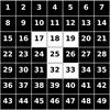 |
Fig. A.1 Illustration of the friend-of-friend algorithm (see Appendix A for details). White and black cells correspond to ionized and neutral cells, respectively. |
Figure A.1, illustrates the algorithm in two dimensions. In this figure, black cells correspond to neutral cell and white cells to ionized cells with an ionized fraction x ≥ 0.5. In this example, 6 cells belongs to the same HII region, with numbers 17, 18, 25, 32, and 33, and all of them should receive the same
identification number. Following the algorithm described above, the cells would be visited in the following order: 17-18-19-18-25-32-33-32-25-18-17. At this stage, when the algorithm recovers the starting cell with all its ionized neighbors marked as visited, it stops.
To implement this method, a recursive scheme could be used, as well as linked lists. We chose the second option since it limits the use of large stacks of memory. We also mention that for boxes of 10243, we have parallelized the identification on the large box by cutting it into 16 sub-boxes. We thus do the identification on this 16 sub-boxes in parallel to accelerate the calculation. We then reassemble the entire box and merge the IDs.
Appendix A.2: Effect of the neutral ionization threshold
The FOF algorithm assumes an ionization threshold in order to decide if a cell is ionized or not. As often used in the literature, we chose a value of x ≥ 0.5 to consider a cell as ionized. To test the impact of the threshold’s value on the identification of the HII regions, we also tried other values for the ionization fraction in the FOF procedure.
Figure A.2 represents the radius distribution of the HII regions for three different instants. The distributions were done for the three models of ionizing sources for the 50 Mpc/h box size. We compared the radius distributions according to three different ionizing thresholds of x ≥ 0.3, x ≥ 0.5, and x ≥ 0.9 to assume that a cell is ionized. The three distributions are very similar for all models and at each instant, regardless of the chosen ionizing threshold. The most significant variation stands for small regions with radius below ~2×10⁻¹ Mpc/h, which are detected in greater numbers with x ≥ 0.9. Meanwhile, the distributions with x ≥ 0.3 and x ≥ 0.5 are almost superimposed in all cases. Additionally, we used the merger tree properties to plot the same distributions in Fig. A.3 but dissociated the contributions of each type of region. This time, we have only represented the distribution for both the x ≥ 0.5 and x ≥ 0.9 ionization thresholds, which previously exhibited the greater difference. We see that for the most part, the families remain unchanged and therefore that the merger tree properties are conserved even when varying the ionization threshold. The only difference is that with x ≥ 0.9 the FOF procedure tends to detect more small recombining regions than with x ≥ 0.5 in the boosted star and star models.
The only remarkable effects by varying the threshold therefore is for high threshold values within recombining regions, which represent a tiny number and volume fraction of the HII regions network. It does not come as a surprise, though, since recombinations occur in already ionized regions, and any fluctuations within, combined with a high detection threshold, lead to a subdivision of regions in smaller ones. One might even consider that such an effect should be avoided since it increases branches in the merging tree with regions that may be short-lived or unstable. As a conclusion, we can thus consider that the value of x ≥ 0.5 used in the paper for identifying the HII regions is a good compromise, in addition to being the one commonly used.
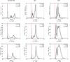 |
Fig. A.2 Representation of the radius distribution of all HII regions at three different redshifts for the three simulations for the 50 Mpc/h box. We compare the difference in the radius distribution according to the ionization threshold for the detection of the HII region with the FOF procedure. We represent the volume of one single cell by the vertical red line. |
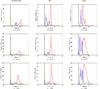 |
Fig. A.3 Radius distribution of all HII regions at three different redshifts for the three simulations for the 50 Mpc/h box. This time, we dissociate the distribution into the different counterparts of the type of HII region considered. We compare the difference in the radius distribution according to both ionization thresholds of x ≥ 0.5 and x ≥ 0.9 for the detection of the HII region with the FOF procedure. The colors stand for the new HII regions (blue), the expanding regions (red), the regions that will recombine (yellow), and the regions resulting from mergers (green). In addition we represent the volume of one single cell by the vertical black line. |
Appendix B: Merger tree algorithm
The implementation of the merger tree algorithm is performed as follows (see also Fig. B.1):
-
1.
We look at an instant t of the simulation where the cells of a particular ionized region are located. They all share the same ID.
-
2.
Then, we extract the same cells at time t + 1. These cells may have different IDs.
-
3.
The most common ID at time t + 1 is kept and is linked to the ID investigated at t.
This scheme is repeated for all HII regions between the snapshot t and t + 1. We finally reproduce this process between each snapshot.
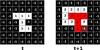 |
Fig. B.1 Merger tree algorithm. All neutral cells are black with an identification number of −1. All ionized cells are white with an identification number. At time t, we have the ionized region identified with an identification number of 1. We look forward to time t + 1 where cells of this ionized region are located (shown in red). Here ID 1 at time t is linked to ID 2 at time t + 1. |
All Figures
|
Fig. 1 Illustration of the merger tree of HII regions. Each black line represents an ID evolution with the redshift for a distinct HII region. For clarity, we represent here only the ID evolution for 30 regions. |
| In the text | |
|
Fig. 2 Illustration of the properties that we can follow with the merger tree. In each diagram, red items symbolize the kinds of properties that we follow. 1: The number of new HII regions between two snapshots; 2: the number of growing ionized regions; 3: the number of HII regions that recombine; 4: the number of HII regions resulting from mergers and, 5: the number of parents involved for an HII region resulting from mergers. |
| In the text | |
|
Fig. 3 Redshift evolution of the cumulative number of ionizing photons emitted by the sources relative to the number of hydrogen atoms. The horizontal line stand for one photon per atom. Solid (resp. dashed) lines stand for the 200 (resp. 50) Mpc/h simulations. Black, blue, and red curve stand respectively for the star, Boosted Star and Halo models of ionizing sources. |
| In the text | |
|
Fig. 4 Evolution of the volume-weighted average ionization fraction with redshift for the six simulations. |
| In the text | |
|
Fig. 5 Evolution of the Thomson optical depth with redshift for the six simulations. |
| In the text | |
|
Fig. 6 Ionization map for the three ionizing sources models for three distinct redshift for the 200 Mpc/h size box. The colors encode the different identification number allocated to the HII regions by the FOF algorithm. |
| In the text | |
|
Fig. 7 Ionization map for the three ionizing sources models for three distinct redshifts for the 50 Mpc/h size box. The colors encode the different identification number allocated to the HII regions by the FOF algorithm. |
| In the text | |
|
Fig. 8 Evolution of the number density of each kind of HII region as a function of redshift for the three models of ionizing sources and for both boxes of 200 and 50 Mpc/h. Panels a)–c) respectively represent the distribution for the Boosted Star, the Star, and the Halo models for the 200 Mpc/h box, while the panels d)–f) are for the same models but for the 50 Mpc/h box. The colors stand for the new HII regions (blue), the expanding regions (red), the regions that will recombine (yellow), and the regions resulting from mergers (green). |
| In the text | |
|
Fig. 9 Evolution of the proportion of each kind of HII regions as a function of redshift for the three models of ionizing sources and for both boxes of 200 and 50 Mpc/h. Panels a)–c) respectively represents the distribution for the Boosted Star, the Star, and the Halo model for the 200 Mpc/h box, while the panels d)–f) are for the same models but for the 50 Mpc/h box. The colors stand for the new HII regions (blue), the expanding regions (red), the regions that will recombine (yellow), and the regions resulting from mergers (green). The black vertical line shows the peak of the absolute number of HII regions: zpeak. |
| In the text | |
|
Fig. 10 Evolution of the volume fraction of each kind of HII regions as a function of redshift for the three models of ionizing sources and for both boxes of 200 and 50 Mpc/h. Panels a)–c) respectively represents the distribution for the Boosted Star, the Star, and the Halo model for the 200 Mpc/h box, while the panels d)–f) are for the same models but for the 50 Mpc/h box. The colors stand for the new HII regions (blue), the expanding regions (red), the regions that will recombine (yellow), and the regions resulting from mergers (green). The black vertical line shows the peak of the absolute number of HII regions: zpeak and the black horizontal line shows the volume fraction of one cell of the grid. |
| In the text | |
|
Fig. 11 Evolution of the HII regions radius distribution as a function of redshift for the three models of ionizing sources formation and for both boxes of 200 and 50 Mpc/h. Panels a)–c) respectively represents the distribution for the Boosted Star, the Star and the Halo model for the 200 Mpc/h box, while the panels d)–f) are for the same models but for the 50 Mpc/h box. The brightest red cells represent the location in the distribution populated by a single HII region, other red tones up to the brightest green cells span distribution densities from a couple of HII regions up to a value corresponding to half the maximum value of the distribution. Finally, the purple tones (from the darkest to the brightest) denote the maximum values. The evolution of the average radius and the evolution of the radius of the main region are shown by the solid and dashed white lines, respectively. |
| In the text | |
|
Fig. 12 Evolution of the radius distribution of each kind of HII regions as a function of redshift for the three models of ionizing source formation and for both boxes of 200 and 50 Mpc/h. Panels a)–c) respectively represents the distribution for the Boosted Star, the Star, and the Halo model for the 200 Mpc/h box, while the panels d)–f) are for the same models but for the 50 Mpc/h box. The colors stand for the new HII regions (blue), the expanding regions (red), the regions that will recombine (yellow), and the regions resulting from mergers (green). In addition the solid and dashed black lines represent the radius evolution of the main region end the evolution of the average radius for the HII regions, respectively. |
| In the text | |
|
Fig. 13 Distribution of the number of parents for the HII regions resulting from merger as a function of redshift for the three kinds of ionizing sources and for both box sizes of 200 and 50 Mpc/h. Panels a)–c) respectively represent the distribution for the Boosted Star, the Star, and the Halo model for the 200 Mpc/h box, while the panels d)–f) are for the same models but for the 50 Mpc/h box. The brightest red cells represent the location in the distribution populated by a single HII region; other red tones up to the brightest green cells span distribution densities from a couple HII regions up to a value corresponding to half the maximum value of the distribution. The purple tones (from the darkest to the brightest) denote the maximum values, and the evolution of the average number of parents and the evolution of the number of parents of the main region are represented with the solid and dashed white lines, respectively. |
| In the text | |
|
Fig. 14 Distribution of the HII regions sizes for the regions that merge with the dominant region as a function of redshift for the three kinds of ionizing sources and for both box sizes of 200 and 50 Mpc/h. Panels a)–c) respectively represent the distribution for the Boosted Star, the Star, and the Halo model for the 200 Mpc/h box, while the panels d)–f) are for the same models but for the 50 Mpc/h box. The brightest red cells represent the location in the distribution populated by a single HII region; other red tones up to the brightest green cells span distribution densities from a couple HII regions up to a value corresponding to half the maximum value of the distribution. The purple tones (from the darkest to the brightest) denote the maximum values. The evolution of the average radius for the regions that merge with the dominant region and the evolution of the radius of the main region are represented with the solid and dashed white lines, respectively. |
| In the text | |
|
Fig. A.1 Illustration of the friend-of-friend algorithm (see Appendix A for details). White and black cells correspond to ionized and neutral cells, respectively. |
| In the text | |
|
Fig. A.2 Representation of the radius distribution of all HII regions at three different redshifts for the three simulations for the 50 Mpc/h box. We compare the difference in the radius distribution according to the ionization threshold for the detection of the HII region with the FOF procedure. We represent the volume of one single cell by the vertical red line. |
| In the text | |
|
Fig. A.3 Radius distribution of all HII regions at three different redshifts for the three simulations for the 50 Mpc/h box. This time, we dissociate the distribution into the different counterparts of the type of HII region considered. We compare the difference in the radius distribution according to both ionization thresholds of x ≥ 0.5 and x ≥ 0.9 for the detection of the HII region with the FOF procedure. The colors stand for the new HII regions (blue), the expanding regions (red), the regions that will recombine (yellow), and the regions resulting from mergers (green). In addition we represent the volume of one single cell by the vertical black line. |
| In the text | |
|
Fig. B.1 Merger tree algorithm. All neutral cells are black with an identification number of −1. All ionized cells are white with an identification number. At time t, we have the ionized region identified with an identification number of 1. We look forward to time t + 1 where cells of this ionized region are located (shown in red). Here ID 1 at time t is linked to ID 2 at time t + 1. |
| In the text | |
Current usage metrics show cumulative count of Article Views (full-text article views including HTML views, PDF and ePub downloads, according to the available data) and Abstracts Views on Vision4Press platform.
Data correspond to usage on the plateform after 2015. The current usage metrics is available 48-96 hours after online publication and is updated daily on week days.
Initial download of the metrics may take a while.