| Issue |
A&A
Volume 548, December 2012
|
|
|---|---|---|
| Article Number | A77 | |
| Number of page(s) | 17 | |
| Section | Interstellar and circumstellar matter | |
| DOI | https://doi.org/10.1051/0004-6361/201219912 | |
| Published online | 26 November 2012 | |
The complete far-infrared and submillimeter spectrum of the Class 0 protostar Serpens SMM1 obtained with Herschel
Characterizing UV-irradiated shocks heating and chemistry⋆,⋆⋆
1
Centro de Astrobiología (CSIC/INTA), Ctra. de Torrejón a Ajalvir, km 4,
28850
Torrejón de Ardoz, Madrid
Spain
e-mail: jr.goicoechea@cab.inta-csic.es
2
Max-Planck-Institut für extraterrestrische Physik (MPE),
Postfach 1312,
85741
Garching,
Germany
3
Leiden Observatory, Leiden University,
PO Box 9513,
2300 RA
Leiden, The
Netherlands
4
Kavli Institute for Astronomy and Astrophysics, Peking University,
Yi He Yuan Lu 5, HaiDian Qu,
100871
Beijing, PR
China
5
RAL Space, Rutherford Appleton Laboratory,
Chilton, Didcot,
Oxfordshire, OX11 0QX, UK
6
Institute for Space Imaging Science, University of Lethbridge,
4401 University Drive, Lethbridge, Alberta
T1J 1B1,
Canada
7
Centre for Star and Planet Formation, Natural History Museum of
Denmark, University of Copenhagen, Øster Voldgade5-7, 1350
København K,
Denmark
8
Université de Toulouse, UPS-OMP, IRAP, Toulouse, France
9
CNRS, IRAP, 9
Av. colonel Roche, BP
44346, 31028
Toulouse Cedex 4,
France
10
Department of Astronomy, University of Michigan,
500 Church St., Ann Arbor, MI
48109,
USA
Received:
28
June
2012
Accepted:
17
September
2012
We present the first complete ~55−671 μm spectral scan of a low-mass Class 0 protostar (Serpens SMM1) taken with the PACS and SPIRE spectrometers onboard Herschel. More than 145 lines have been detected, most of them rotationally excited lines of 12CO (full ladder from Ju = 4−3 to 42−41 and Eu/k = 4971 K), H2O (up to 818−707 and Eu/k = 1036 K), OH (up to 2Π1/2 J = 7/2−5/2 and Eu/k = 618 K), 13CO (up to Ju = 16−15), HCN and HCO+ (up to Ju = 12−11). Bright [O i]63, 145 μm and weaker [C ii]158 and [C i]370, 609 μm lines are also detected, but excited lines from chemically related species (NH3, CH+, CO+, OH+ or H2O+) are not. Mid-infrared spectra retrieved from the Spitzer archive are also first discussed here. The ~10−37 μm spectrum has many fewer lines, but shows clear detections of [Ne ii], [Fe ii], [Si ii] and [S i] fine structure lines, as well as weaker H2 S(1) and S(2) pure rotational lines. The observed line luminosity is dominated by CO (~54%), H2O (~22%), [O i] (~12%) and OH (~9%) emission. A multi-component radiative transfer model allowed us to approximately quantify the contribution of the three different temperature components suggested by the 12CO rotational ladder (Tkhot ≈ 800 K, Tkwarm ≈ 375 K and Tkcool ≈ 150 K). Gas densities n(H2) ≳ 5 × 106 cm-3 are needed to reproduce the observed far-IR lines arising from shocks in the inner protostellar envelope (warm and hot components) for which we derive upper limit abundances of x(CO) ≲ 10-4, x(H2O) ≲ 0.2 × 10⁻⁵ and x(OH) ≲ 10-6 withrespect to H2. The lower energy submm 12CO and H2O lines show more extended emission that we associate with the cool entrained outflow gas. Fast dissociative J-shocks (vs > 60 km s-1) within an embedded atomic jet, as well as lower velocity small-scale non-dissociative shocks (vs ≲ 20 km s-1) are needed to explain both the atomic fine structure lines and the hot CO and H2O lines respectively. Observations also show the signature of UV radiation (weak [C ii] and [C i] lines and high HCO+/HCN abundance ratios) and thus, most observed species likely arise in UV-irradiated shocks. Dissociative J-shocks produced by a jet impacting the ambient material are the most probable origin of [O i] and OH emission and of a significant fraction of the warm CO emission. In addition, H2O photodissociation in UV-irradiated non-dissociative shocks along the outflow cavity walls can also contribute to the [O i] and OH emission.
Key words: stars: protostars / ISM: jets and outflows / infrared: ISM / shock waves
Herschel is an ESA space observatory with science instruments provided by European-led Principal Investigator consortia and with important participation from NASA.
Appendix A is available in electronic form at http://www.aanda.org
© ESO, 2012
1. Introduction
In the earliest stages of evolution, low-mass protostars are deeply embedded in dense envelopes of molecular gas and dust. During collapse, conservation of angular momentum combined with infall along the magnetic field lines leads to the formation of a dense rotating protoplanetary disk that drives the accretion process. At the same time, both mass and angular momentum are removed from the system by the onset of jets, collimated flows, and the magnetic braking action (e.g., Bontemps et al. 1996; Bachiller & Tafalla 1999). The resulting outflow produces a cavity in the natal envelope with walls subjected to energetic shocks and strong radiation fields from the protostar. These processes heat the circumstellar gas and leave their signature in the prevailing chemistry (e.g., enhanced abundances of water vapour).
Both the line and continuum emission from young stellar objects (YSOs) peak in the far-infrared (far-IR) and thus they are robust diagnostics of the energetic processes associated with the first stages of star formation (e.g., Giannini et al. 2001). The improved sensitivity and angular/spectral resolution of Herschel spectrometers compared to previous far-IR observatories allows us to detect a larger number of far-IR lines and to better constrain their spatial origin. This is especially true for the detection of high excitation, optically thin lines that can help us to identify high temperature components as well as to disentangle and quantify the dominant heating mechanisms (mechanical vs. radiative). Early Herschel observations of a few low-mass protostars for which partial or complete PACS spectra are available show that the molecular emission of relatively excited 12CO (J < 30), H2O and OH lines is a common feature (van Kempen et al. 2010 for HH46; and Benedettini et al. 2012 for L1157-B1). This warm CO and H2O emission was suggested to arise from the walls of an outflow-carved cavity in the envelope, which are heated by UV photons and by non-dissociative C-type shocks (van Kempen et al. 2010; Visser et al. 2012). The [O i] and OH emission observed in these sources, however, was proposed to arise from dissociative J-shocks. Herczeg et al. (2012) detected higher-J12CO lines (up to J = 49−48) and highly excited H2O lines in the NGC 1333 IRAS 4B outflow indicating the presence of even hotter gas. The very weak [O i]63 μm line emission in IRAS 4B outflow (the [O i]145 μm line is not even detected) led these authors to conclude that the hot gas where H2O dominates the gas cooling is heated by non-dissociative C-shocks shielded from UV radiation. Passive heating by the protostellar luminosity is also thought to contribute to the mid-J 12CO and 13CO emission (Visser et al. 2012; Yıldız et al. 2012). In NGC 1333 IRAS 4A/4B, however, the 12CO intensities and broad line-profiles of lower-J transitions (J = 1−0 up to 10−9) probe swept-up or entrained shocked gas along the outflow (Yıldız et al. 2012).
In this paper we present the first complete far-IR and submm spectra of a Class 0 protostar (Serpens SMM1 or FIRS 1), taken with the PACS (Poglitsch et al. 2010) and SPIRE (Griffin et al. 2010) spectrometers onboard the Herschel Space Observatory (Pilbratt et al. 2010). SMM1 is a low-mass protostellar system located in the Serpens core (Eiroa et al. 2008) at a distance of d = 230 ± 20 pc (see also Dzib et al. 2010, for an alternative measurement). It is the most massive low-mass Class 0 source (Menv ≃ 16.1 M⊙, Tbol ≃ 39 K) of the WISH program sample (Water in Star-forming Regions with Herschel, van Dishoeck et al. 2011). The Herschel spectra are complemented with mid-IR Spitzer Infrared Spectrograph (IRS) archive spectra of the embedded protostar (photometry first presented by Enoch et al. 2009).
The Serpens cloud core was first mapped in the far-IR with the LWS spectrometer onboard the Infrared Space Observatory (ISO). Even with a poor angular and spectral resolution of ~80′′ and R = λ/Δλ ~ 200, ISO-LWS observations of Serpens SMM1 revealed a rich spectrum of molecular lines (Larsson et al. 2002), superposed onto a strong far-IR continuum (Larsson et al. 2000). In particular, 12CO (up to J = 21−20), H2O (up to 441−330) and some OH lines were detected. Detailed modeling of the ISO emission concluded that those species trace the inner ~103 AU regions around the protostar, where gas temperatures are above 300 K and densities above 106 cm-3. The comparison of the H2O, OH and CO lines with existing shock models suggested that shock heating along the SMM1 outflow is the most likely mechanism of molecular excitation. The details of these shocks, however, were less clear.
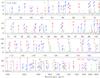 |
Fig. 1 PACS and SPIRE (lower panel) continuum-subtracted spectra of Serpens SMM1 (central spaxel) with H2O (blue), CO (red), OH (cyan), 13CO (magenta), [O i], [C ii] and [C i] (green), and HCO+ and HCN (black) lines labelled. The flux density scale is in Jy (assuming a point source). |
Because of its far-IR luminosity and rich spectrum, Serpens SMM1 is an ideal Class 0 source for studying the protostellar environment and to characterize the shock- and UV-heating and chemistry with the much higher spatial and spectral capabilities provided by Herschel. In the following sections we present the data set, we identify the observed lines, present a 3 component non-local thermodynamic equilibrium (non-LTE) radiative transfer model and compare the observations with available shock models and observations of other YSOs.
2. Observations and data reduction
2.1. Herschel PACS and SPIRE observations
PACS spectra between ~55 and ~210 μm were obtained on 31 October 2010 in the range spectroscopy mode. The PACS spectrometer uses photoconductor detectors and provides 25 spectra over a 47′′ × 47′′ field-of-view (FoV) resolved in 5 × 5 spatial pixels (“spaxels”), each with a size of ~9.4′′ on the sky. The resolving power varies between R ~ 1000 (at ~100 μm in the R1 grating order) and ~5000 (at ~70 μm in the B3A order). The central spaxel was centered at the Serpens SMM1 protostar (α2000: 18h29m49.8s, δ2000: 1°15′20.5′′). Observations were carried out in the “chop-nodded” mode with the largest chopper throw of 6 arcmin. The total observing time was ~3 h (observation IDs 1342207780 and 1342207781). The measured width of the spectrometer point spread function (PSF) is relatively constant for λ ≲ 100 μm (FWHM ≃ spaxel size) but increases at longer wavelengths. In particular only ≃40% (≃70%) of a point source emission would fall in the central spaxel at ≃190 μm (λ ≃ 60 μm). Hence, extracting line surface brightness from a semi-extended source like Serpens SMM1 is not trivial. In this work we followed the method described by Herczeg et al. (2012) and Karska et al. (2012). This involves multiplying all line fluxes measured in the central spaxel with a λ-dependent correction curve calculated from the extended emission of the brightest CO and H2O lines observed over the entire FoV. The correction factor is constant (~2) for λ < 120 μm and increases from ~2 to ~3−4 at ~200 μm. For the continuum and [O i] and [C ii] lines, the individual line fluxes measured in all spaxels were added. Note that we checked that the reference spectra in the two off positions are free of [C ii] emission to confirm that the [C ii] lines towards Serpens SMM1 are real. Figure 1 shows the PACS spectrum in the central spaxel and Fig. 2 shows the entire PACS array from 55 to 190 μm (the bright emission line is [O i]63 μm).
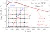 |
Fig. 2 Observed spectral energy distribution (SED) of Serpens SMM1 and modified blackbody fit (red curve). Inset shows the full PACS array in flux density units of 10-14 W m-2 μm-1. The abscissa is in linear scale from 55 to 190 μm. The bright emission line seen in several positions is [O i]63 μm. Approximate outflow directions are shown with red and blue arrows. |
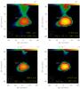 |
Fig. 3 Upper: SPIRE-FTS 12CO J = 9−8 and 12−11 sparse maps. Lower: p-H2O 111–000 and 202–111 maps respectively. The line surface brightness is on the 10-8 W m-2 sr-1 scale. The white contours represent the 50% line emission peak level. The FWHM beam is shown in each inset. Note the increase of line surface brightness in the more excited lines. |
SPIRE FTS spectra between ~194 and ~671 μm (1545−447 GHz) were
obtained on 27 March 2011. The SPIRE FTS uses two bolometer arrays covering the
194−313 μm (short wavelength array, SSW) and
303−671 μm (long wavelength array, SLW) bands. The two arrays contain
19 (SLW) and 37 (SSW) hexagonally packed detectors separated by ~2 beams
(51′′ and 33′′ respectively). The unvignetted FoV is
~2′. The observation was centered at Serpens SMM1 (IDs 1342216893) in the
high spectral resolution mode ( = 0.04 cm-1;
R ~ 500−1000). The total integration time was ~9 min. We
corrected the spectrum to account for the extended continuum and molecular emission of the
source and the changing beam size with frequency across the SPIRE band. Taking account of
the coupling of the source to the SPIRE-FTS beam (Wu et al., in prep.) and using the
overlap region between the SSW and SLW bands as a reference (where the beam size differs
by a factor of ~2) we calculate the FWHM size of the submm continuum source to
be ~20′′. The SPIRE continuum fluxes were appropriately corrected and the
unapodized spectrum was used to fit the line intensities with sinc functions. Four
representative mid-J12CO and H2O integrated line
intensity maps are shown in Fig. 3.
= 0.04 cm-1;
R ~ 500−1000). The total integration time was ~9 min. We
corrected the spectrum to account for the extended continuum and molecular emission of the
source and the changing beam size with frequency across the SPIRE band. Taking account of
the coupling of the source to the SPIRE-FTS beam (Wu et al., in prep.) and using the
overlap region between the SSW and SLW bands as a reference (where the beam size differs
by a factor of ~2) we calculate the FWHM size of the submm continuum source to
be ~20′′. The SPIRE continuum fluxes were appropriately corrected and the
unapodized spectrum was used to fit the line intensities with sinc functions. Four
representative mid-J12CO and H2O integrated line
intensity maps are shown in Fig. 3.
SPIRE and PACS data were processed using HIPE and then exported to GILDAS where basic line spectrum manipulations were carried out. Table A.1 summarize the detected lines and the line fluxes towards the protostar position (central spaxel; corrected for extended emission in the case of PACS observations). The spatial distribution of several atomic and molecular lines observed in the PACS array is shown in Fig. 4.
2.2. Spitzer IRS Observations
In order to complement the far-IR and submm Herschel spectra we have also analyzed mid-IR data towards the protostar position from the Infrared Spectrograph (IRS) onboard Spitzer (Houck et al. 2004) in high spectral resolution mode (R ~ 600; 9.9−37.2 μm). The basic calibrated data (BCD) files for the short high (SH) and long high (LH) orders of IRS were retrieved from the Spitzer Heritage Archive1 (OBSID 34330, PI M. Enoch). Pipelining of the data was achieved using CUBISM (Smith et al. 2007) to assemble the BCD files into spectral cubes. Bad and rogue pixels were removed using 3-sigma filtering. The spectra were extracted in a ~7′′ × 7′′ aperture, thus close to the PACS spaxel size. The resulting Spitzer IRS spectra are shown in Fig. 5. The photometry of these data was first presented by Enoch et al. (2009). Table A.2 summarizes the detected lines and their fluxes.
3. Results
3.1. Far-infrared and submillimeter lines
Figure 1 shows the very rich PACS and SPIRE (lower
panel) spectrum of the Serpens SMM1 protostar. More than 145 lines have been detected,
most of them rotationally excited lines from abundant molecules: 38 12CO lines
(up to J = 42−41 and
Eu/k = 4971 K), 37 lines of both
o-H2O and p-H2O (up to
818−717 and
Eu/k = 1036 K), 16 OH lines (up to
 J =
7/2−5/2 and Eu/k = 618 K),
12 13CO lines (up to J = 16−15 and
Eu/k = 719 K) and several HCN and
HCO+ lines (up to J = 12−11 and
Eu/k = 283 K). Weaker
[C ii]158 μm and [C i]370, 609 μm
lines are also detected. Excited lines from NH3, CH+,
CO+, OH+ or H2O+ are however not detected at
the PACS and SPIRE spectral resolutions and sensitivity. The brightest line in the spectra
is the [O i]63 μm line (see also Fig. 2) with a luminosity of L63 ≃
0.014 L⊙. Assuming no extinction in the far-IR, we measure
[O i]63 μm/[C ii]158 μm ≃ 30 and
[O i]63 μm/[O i]145 μm ≃ 10 line
flux ratios integrated over the entire PACS array.
J =
7/2−5/2 and Eu/k = 618 K),
12 13CO lines (up to J = 16−15 and
Eu/k = 719 K) and several HCN and
HCO+ lines (up to J = 12−11 and
Eu/k = 283 K). Weaker
[C ii]158 μm and [C i]370, 609 μm
lines are also detected. Excited lines from NH3, CH+,
CO+, OH+ or H2O+ are however not detected at
the PACS and SPIRE spectral resolutions and sensitivity. The brightest line in the spectra
is the [O i]63 μm line (see also Fig. 2) with a luminosity of L63 ≃
0.014 L⊙. Assuming no extinction in the far-IR, we measure
[O i]63 μm/[C ii]158 μm ≃ 30 and
[O i]63 μm/[O i]145 μm ≃ 10 line
flux ratios integrated over the entire PACS array.
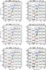 |
Fig. 4 PACS spectral maps of Serpens SMM1 in the o-H2O
303–212 (174.626 μm);
[C ii]157.741 μm; CO J = 17−16
(153.267 μm); both
p-H2O 322–211
(89.988 μm) and CO J = 29−28
(90.163 μm); [O i]63.183 μm and OH
|

Most of the far-IR continuum and line emission arises from the protostar position (central spaxel) with weaker, but detectable, contributions from adjacent outflow positions (see Fig. 4). In particular, the high excitation lines of CO, H2O and OH detected below λ < 100 μm seem to show a more compact distribution than the lower excitation lines (within the PACS PSF sampling caveats). The highest PACS spectral resolution (~90−60 km s-1) is achieved in the ~60−70 μm range. Although at this resolution all detected molecular lines are spectrally unresolved (they have narrower intrinsic line-widths), the observed [O i]63 μm line is >30% broader than any close-by molecular line in the ~60−70 μm range. This likely indicates that PACS marginally resolves the [O i]63 μm line, being broader (or having higher velocity line-wing emission) than the excited far-IR CO, H2O and OH lines. In addition, the [O i]63 μm line-profile peak shifts in velocity from the protostar position (where the line is brightest) to the outflow red-lobe position where the line peak is redshifted by ~100 km s-1 (more than a resolution element) and the molecular line emission is weaker (see red boxes in Fig. 4). Note that [C ii]158 μm peaks at this red-lobe position and the line peak is also redshifted by ~100 km s-1 (although less than a resolution element in this wavelength range). Similar [O i]63 μm velocity-shifts are also seen in sources such as HH46 and are associated with the emission from an atomic jet itself (van Kempen et al. 2010). We refer to Karska et al. (2012) for a detailed comparison of the [O i]63 μm shifts in several outflows.
Finally, the lower energy submm lines, from 12CO and H2O in particular, show a more extended distribution than the far-IR lines, with some indication of outflow emission in the the S-E direction (see SPIRE maps in Fig. 3).
Table 1 summarizes the total line luminosities adding all observed lines between ~55 and 671 μm. Note that a few unidentified lines (U) are present in the PACS spectrum.
3.2. Mid-infrared lines and extinction
The mid-IR spectrum of Serpens SMM1 (Fig. 5a) shows a much less rich spectrum than in the far-IR domain (probably due to severe dust extinction and lack of spectral resolution). Nevertheless, two weak H2 pure rotational lines (0−0 S(1) and S(2) transitions) and seven brighter atomic fine-structure lines of Ne+, Si+, S and Fe+ (four transitions) are clearly detected2 at the protostar position (Figs. 5b and c). In contrast with NGC 1333-IRAS 4B (Watson et al. 2007), no mid-IR OH and H2O lines are seen. The presence of [Ne ii] and [Fe ii] lines from energy levels above a few thousands Kelvin, together with the bright and velocity-shifted [O i] line detected by Herschel, suggests the presence of fast dissociative shocks close to the protostar (e.g., Hollenbach & McKee 1989; Neufeld & Dalgarno 1989). Note that the same mid-IR lines are readily detected in Herbig-Haro objects and outflow lobes (e.g., Neufeld et al. 2006; Melnick et al. 2008). As discussed in Sect. 4, the observed intensities of H2, H2O and CO rotational lines are more typical of slower velocity shocks.
The large amount of gas and dust in embedded YSOs requires to apply extinction corrections to retrieve corrected mid-IR line luminosities. In this work we have taken grain optical properties from Laor & Draine (1993) and computed an extinction curve A(λ)/AV from IR to submm wavelengths characterized by RV = AV/E(B − V) = 5.5 (the ratio of visual extinction to reddening) and a conversion factor from extinction to hydrogen column density of 1.4 × 1021 cm-2 mag-1. These values have been previously used to correct photometric observations of embedded YSOs in the Serpens cloud (Evans et al. 2009). Table 1 lists the uncorrected mid-IR line luminosities and those using an arbitrary correction of AV = 150. In the latter case, even the [O i]63 μm line would be affected by extinction (the de-reddened line flux would be ~2 times higher) and the [O i]63/145 μm line flux ratio would increase to ~20. Such large intensity ratios are predicted by dissociative shocks models (e.g., Hollenbach & McKee 1989; Neufeld & Dalgarno 1989; Flower & Pineau Des Forêts 2010) and thus provide a reasonable upper value to the extinction in the inner envelope.
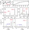 |
Fig. 5 a) Spitzer IRS spectrum of the Class 0 protostar Serpens SMM1 using the Hi Res modules and a 7′′ × 7′′ aperture. b) Continuum-subtracted spectra with main narrow lines identified in the LH module (λ ≥ 19.5 μm) and c) with the SH module (λ ≤ 19.5 μm). Note the lack of bright molecular line emission (H2O, OH, etc.). |
Observed and modelled luminosities.
An independent estimate of the extinction is obtained from the ~9.7 μm silicate grains absorption band seen in the Spitzer IRS low resolution spectra (shown in Enoch et al. 2009). In the diffuse ISM, the optical depth of the ~9.7 μm broad feature is proportional to AV (e.g., Whittet 2003). Although it is not clear that the same correlation holds in the dense protostellar medium (Chiar et al. 2007), we computed a lower limit to the extinction of AV ≳ 30 by fitting the ~9.7 μm absorption band and assuming a single slab geometry.
3.3. Dust continuum emission
The dust continuum emission peaks in the far-IR domain at ~100 μm. This is consistent with the presence of a massive dusty envelope with relatively warm dust temperatures. Using a simple modified blackbody with a dust opacity varying as τλ = τ100(100/λ)β, where τ100 is the continuum opacity at 100 μm and β is the dust spectral index, we obtain a size of ~7′′ for the optically thick far-IR continuum source, with τ100 ≃ 2.5, β = 1.7, Lfar−IR ≃ 26 L⊙ and a dust temperature of Td ≃ 33 K (Fig. 2). These parameters agree with more sophisticated radiative transfer models of the continuum emission detected with ISO/LWS, for which a far-IR source size of ~4′′ (~500 AU in radius) and Td = 43 K at the τ100 = 1 equivalent radius were inferred (Larsson et al. 2000). They are also consistent with more recent SED models (Kristensen et al. 2012) and with the compact (~5′′) emission revealed by mm interferometric observations and thought to arise from the densest regions of the inner envelope and from outflow material (Hogerheijde et al. 1999; Enoch et al. 2009). Note that owing to the large continuum opacity below 100 μm, observations at these wavelengths probably do not trace the innermost regions, i.e., the developing circumstellar disk with an approximate radius of ~100 AU (e.g., Rodríguez et al. 2005).
4. Analysis
4.1. 12CO, 13CO, H2O and OH Rotational Ladders
Figure 6 shows all 12CO and 13CO detected lines in a rotational diagram. In this plot we assumed that the line emission arises from a source with a radius of 500 AU (see Sect. 3.3). Given the high densities in the inner envelope of protostars (>106 cm-3; see below), the rotational temperatures (Trot) derived from these plots are a good lower limit to Tk. The 12CO diagram suggests the presence of 3 different Trot components with Trot = 622 ± 30 K (for Ju ≲ 42), Trot = 337 ± 40 K (Ju ≲ 26) and Trot = 103 ± 15 K (Ju ≲ 14) respectively. The estimated error in Trot corresponds to different choices of Ju cutoffs for the different components3. In the following we shall refer to them as the hot, warm and cool components. Whether or not these Trot components are associated with 3 real physical components or with a more continuous temperature and mass distribution will be discussed in Sect. 4.1. Here we note that the submm low-J CO emission shows broad line-profiles and a more extended distribution (Davis et al. 1999; Dionatos et al. 2010) than the high-J CO and H2O lines detected with PACS (more sharply peaked near the protostar). In addition, velocity-resolved observations with HIFI of high-J CO lines up to J = 16−15 show different profiles compared with low-J CO lines (Yıldız et al. 2012; Kristensen et al., in prep.). Specifically, for the 12CO J = 10−9 profile toward SMM1, Yıldız et al. (in prep.) find that about 1/3 of the integrated intensity is due to a narrow (FWHM of a few km s-1) component originating from the quiescent envelope and 2/3 to the broad outflow component. Thus, the cool gas component seen in the SPIRE submm maps is dominated by the entrained outflow gas. On the other hand, the CO J = 16−15 profile of SMM1 is less broad and more similar to the excited H2O line profiles observed with HIFI (Kristensen et al., in prep.). Thus, the far-IR CO and H2O lines detected by PACS clearly probe different physical components than the SPIRE data.
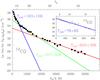 |
Fig. 6 12CO and 13CO rotational diagrams obtained from PACS and SPIRE spectra. The estimated error in Trot for 12CO corresponds to different choices of Ju cutoffs for the different components. The range of possible Trot for 13CO reflects the standard error on the fitted values. |
Alternatively, Neufeld (2012) pointed out that the shape of the rotational diagrams do not, by themselves, necessarily require multiple temperature components. In particular, a single-Trot solution could be found for the 12CO Ju > 14 lines in Serpens SMM1 if the gas were very hot (Tkin ≃ 2500 K) but had a low density (a few 104 cm-3). This scenario seems less likely, at least for the circumstellar gas in the vicinity of the protostar. Note that the gas density in the inner envelope of SMM1 is necessarily higher, as probed by our detection of high-J lines from high dipole moment molecules such as HCN and HCO+ (with very high critical densities). In addition, detailed SED models predict densities of n(H2) ≃ 4 × 106 cm-3 at ~1000 AU, whereas densities of the order of ~105 cm-3 are only expected at much larger radii (Kristensen et al. 2012). Therefore, it seems more likely that the different Trot slopes probe different physical components or the presence of a temperature gradient.
A rotational diagram of the detected 13CO lines provides Trot = 76 ± 6 K, thus lower than the Trot inferred for 12CO in the cool component. The measured 12CO/13CO J = 5−4 line intensity ratio is ≃8, thus much lower than the typical 12C/13C isotopic ratio of ~60 Langer & Penzias (1990), whereas the 12CO/13CO J = 16−15 intensity ratio is ≃55. These different ratios show that the submm 12CO low- and mid-J lines are optically thick, but the high-J far-IR lines are optically thin.
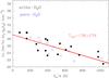 |
Fig. 7 H2O rotational diagram showing o-H2O (filled circles) and p-H2O far-IR lines (open circles). Owing to subthermal excitation (Trot ≪ Tk) and large opacities of most lines, the H2O diagram displays a larger scatter (standard error on the fitted values are shown) than CO. |
An equivalent plot of the observed far-IR H2O line intensities in a rotational diagram gives Trot = 136 ± 27 K without much indication of multiple Trot components (Fig. 7). Since H2O critical densities are much higher than those of CO, collisional thermalization only occurs at very high densities (>108 cm-3). Therefore, the large scatter of the H2O rotational diagram is a consequence of subthermal excitation conditions (Trot ≪ Tk) and large H2O line opacities. We anticipate here that the opacity of most (but not all) far-IR H2O lines is very high (τ ≫ 1). Compared to CO, the H2O rotational diagram is thus obviously less meaningful. A similar rotational diagram of the observed OH lines provides Trot = 72 ± 8 K (see also Wampfler et al. 2012), even lower than the inferred H2O rotational temperature. Like H2O, OH transitions also have high critical densities and line opacities (except the high-energy and the cross-ladder transitions).
4.2. Simple model of the far-IR and submm line emission
Observations and models of the protostellar environment suggest that the observed emission can arise from different physical components, where different mechanisms dominate the gas heating and the prevailing chemistry: hot and warm gas from energetic shocks in the inner envelope (e.g., small scale shocks along the outflow cavity walls, bow shocks and working surfaces within an atomic jet); UV-illuminated gas in the cavity walls; cooler gas from the envelope passively heated by the protostar luminosity and the entrained outflow gas (e.g., van Dishoeck et al. 2011). Unfortunately, the lack of enough spectral and angular resolution of our data does not allow us to provide a complete characterization of all the different possible components. However, the large number of detected lines, high excitation (Eu/k > 300 K) optically thin lines in particular, helps to determine the dominant contributions and the average physical conditions.
With this purpose, we have carried out a non-LTE radiative transfer model of the central spaxel far-IR and submm spectrum (the protostar position) using a multi-molecule LVG code (Cernicharo 2012). In this model we included three spherical components suggested by the three temperature components seen in the 12CO rotational diagram (i.e., hot, warm and cool components). In our model, CO is present in the three components, but since a single rotational temperature roughly explains the observed far-IR H2O and OH lines, most of their emission in the PACS domain can be reproduced with only one component, the hot component for H2O and the warm component for OH (see next section for more details). Note that we do not model the extended quiescent envelope with the bulk of the (cold) mass seen in the mm continuum and narrow C18O line emission (Yıldız et al., in prep.). Foreground absorption and emission from the low density and low temperature extended envelope are thus not included in the model but they will basically influence narrow velocity ranges of the lowest energy-level lines.
The latest available collisional rates were used (e.g., Daniel et al. 2011, and references therein for H2O; and Yang et al. 2010; extended by Neufeld 2012, for CO). Although only one line of o-H2 and one line of p-H2 are detected towards the Serpens SMM1 protostar position, the large H2 0−0 S(2)/S(1) line intensity ratio suggests a H2ortho-to-para (OTP) ratio lower than 3 in the gas probed by these low excitation H2 lines. Here we shall adopt an OTP ratio for H2 of 1 (the value we obtain from the two observed H2 lines assuming LTE and a rotational temperature of ~800 K). Note that such low non-equilibrium H2 OTP values have been inferred, for example, in the hot shocked gas towards HH54 and HH7-11 (Neufeld et al. 2006). The water vapour OTP ratio in the model, however, is let as a free parameter.
The o-H2O ground-state line observed with HIFI towards
Serpens SMM1 shows a two component emission line profile with a medium
component (Δv ≃ 15 km s-1) thought to arise from
small-scale shocks in the inner cavity walls and a broad component
(Δv ≃ 40 km s-1) from more extended shocked-gas along the
outflow (Kristensen et al. 2012). In addition,
velocity-resolved observations of the OH J =
3/2−1/2 line (~163.1 μm) with HIFI show a broad line-profile with
Δv ≃ 20 km s-1 (Wampfler 2012, priv. comm.).
For simplicity here we shall adopt a typical line-width of 20 km s-1 in all
modelled components. As in any LVG calculation, the model is more accurate for
(effectively) optically thin lines (high-J CO lines, excited and weak
H2O and OH lines, etc.) than for very opaque lines (e.g., low
excitation lines).
4.2.1. Model: hot and warm component
Following Sect. 3.3. and previous far-IR studies of this source, we have assumed a size of ~4′′ (~500 AU in radius; e.g., Larsson et al. 2000; Kristensen et al. 2012) for the far-IR source (hot and warm components), a mixture of shocked and UV-illuminated gas (see Sect. 5). A good fit to the high-J12CO emission is obtained for n(H2) ≈ 5 × 106 cm-3 with Tk ≃ 800 K and ≃ 375 K for the hot and warm components respectively. The approximate mass in these components is only M ≲ 0.03 M⊙. Although this solution is not unique, this model satisfactorily reproduces not only the 12CO high-J lines but also the lines from other species (note that we searched for a combination of Tk and n(H2) that reproduces all species simultaneously; see below).
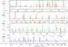 |
Fig. 8 Synthetic non-LTE LVG spectrum of the Class 0 protostar Serpens MM1 convolved to PACS (top three panels) and SPIRE (lower panel) spectral resolutions. Continuous curves show the line emission contribution from the “hot” (red), “warm” (green) and “cool” (blue) components discussed in the text. Vertical labels mark the wavelength position of CO (red), H2O (blue), OH (cyan), 13CO (magenta), HCO+ and HCN (grey) rotational transitions. [O i]63, 145 and [C i]370, 609 μm fine structure lines are marked with green labels. |
In order to constrain the density and place H2O and OH in a particular model
component, we first run a grid of excitation models and investigated how particular line
ratios change with n(H2) and Tk.
In this comparison we choose faint, low-opacity lines arising from high energy levels
that are observed with a similar PSF. Figure A.1
shows the variation of the o-H2O
330–303/615–305
(67.269/82.031 μm) and p-H2O
606–515/515–404
(83.284/95.627 μm) line ratios. The former ratio shows that the
excited H2O lines arise from dense gas, whereas the latter requires high
temperatures (>500 K). The intersection of the two line ratios
is consistent with densities higher than a few 106 cm-3 and
temperatures around ~800 K. Note that for
Tk < 400 K, the predicted
emission from many excited H2O lines below ~100 μm would
be too faint. On the other hand, Fig. A.2 shows a
very clear dependence of the OH 65.279/96.363 μm line ratio with the
gas temperature. The observed ratio does suggest that OH arises from gas at
Tk ≲ 400 K. Following the previous excitation analysis,
and according to the higher observed rotational temperatures
( >
>
 ) and higher
H2O energy levels detected, we placed H2O in the hot
component and OH (together with [O i]) in the warm
component. Although this choice provides a better fit to the data, we can not
obviously conclude that the bulk of the water vapour and OH emission arise from
different physical components.
) and higher
H2O energy levels detected, we placed H2O in the hot
component and OH (together with [O i]) in the warm
component. Although this choice provides a better fit to the data, we can not
obviously conclude that the bulk of the water vapour and OH emission arise from
different physical components.
Far-IR radiative pumping is not included in our models and thus the derived H2O and OH column densities might be considered as upper limits. Nevertheless, all H2O and OH lines are observed in emission and show Trot > Td (where Td is the dust temperature inferred from the SED analysis, see Sect. 3.3), suggesting that owing to the high densities but moderate far-IR radiation field at ≳500 AU, collisions dominate at first order. Note that high-mass protostars produce much stronger far-IR dust continuum fields (by orders of magnitude) and many far-IR OH and water vapour lines are often observed in absorption or show P-Cygni profiles when far-IR pumping dominates the excitation (see e.g., Goicoechea et al. 2006; Cernicharo et al. 2006, for far-IR OH and H2O lines in Orion KL outflows).
4.2.2. Model: cool gas component
In order to fit the more extended 12CO low- and mid-J emission and to match the Trot ≃ 100 K component seen in the 12CO rotational diagram (Fig. 6), we included a third cool component – the entrained outflow gas. From the SPIRE 12CO maps we infer an approximate radius of ~20′′ (~4500 AU) for the emitting region. For this geometry, a density of n(H2) ≈ 2 × 105 cm-3 and a temperature of Tk ≃ 140 K produces a good fit of the observed 12CO submm emission (see also Yıldız et al. 2012, for velocity-resolved observations in NGC 1333 IRAS 4A/4B). This component is also needed to fit the lower excitation H2O submm lines.
Low- and mid-J13CO lines are optically thin and thus, in addition to the swept-up or entrained outflow gas, velocity-resolved submm 13CO line profiles would carry information about other components such as the UV-heated gas and the quiescent envelope, which may well dominate the 13CO lower-J emission (Yıldız et al. 2012). Detailed models of the emission from the extended and passively heated envelope (having most of the mass) predict 12CO rotational temperatures around ≃30−60 K (Visser et al. 2012; Harsono et al., in prep.).
To summarize, Table 2 shows the model parameters and Fig. 8 shows the entire ~55 to 671 μm synthetic spectrum for the hot (red), warm (green) and cool (blue) components convolved with the PACS and SPIRE resolutions. A comparison of the resultant synthetic spectrum (by simply adding the 3 component spectra) with the Herschel spectra is shown in Fig. 9.
4.2.3. Columns, abundances and validity of the model
Owing to the lack of angular resolution to determine the beam filling factors of the different physical components towards Serpens SMM1, the relative abundance ratios derived from the model and shown in Table 3 are a better diagnostic tool than the absolute column densities. Nevertheless, here we provide the source-averaged column densities (N) in the different components as well as the upper limits for several non-detected species (Table 2). In the hot component we find ~5 × 1016 cm-2 and ~2 × 1016 cm-2 column densities for 12CO and H2O respectively. Note that a water vapour OTP ratio of ~3 provides the best fit to the observed water vapour lines and this is the value adopted in the models. Assuming that the gas in the warm component (Tk ≃ 375 K) covers a similar area, we obtain N(OH) ~ 1016 cm-2 and N(12CO) ~ 1018 cm-2 (a factor ≈ 20 larger than N(12CO) in the hot component).
Model components and source-averaged column densities.
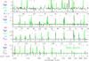 |
Fig. 9 Herschel far-IR and submm spectrum of Serpens SMM1 at the central spaxel position (black histogram) and complete model (green continuous curves) adding the emission from the hot, warm and cool components and convolved to PACS and SPIRE spectral resolutions. |
The detected mid-IR H2 lines provide a lower limit to the H2 column density of NH2 ≈ 1022 cm-2. We use this column density to provide an upper limit to the absolute abundances (with respect to H2) in the hot+warm components. In particular we obtain ≲10-4, ≲0.2 × 10⁻⁵ and ≲10-6 for the CO, H2O and OH abundances respectively. The inferred upper limit to the water vapour abundance is much higher than the ≈ 10−(8−9) value typically found in cold interstellar clouds (e.g., Caselli et al. 2010) but is lower than the ≈ 10-4 value often expected in the hot shocked gas (e.g., Kaufman & Neufeld 1996). Note that the high source-averaged column density of atomic oxygen (~1018 cm-2) suggests that a significant fraction of gas-phase oxygen reservoir in shocks is kept in atomic form.
The column densities in the entrained outflow gas (cool component at Tk ≃ 140 K) are given in Table 2. The absolute columns are more uncertain as they depend on the assumed spatial distribution of the swept-up outflow gas. Note that in order to fit the low-J13CO lines in the cool component, we had to include a low 12CO/13CO column density ratio of ≃10, confirming that the low-J12CO lines are optically thick and thus they do not probe the bulk of the material seen in the low-J CO isotopologue line emission (i.e., the massive and quiescent envelope).
Selected abundance ratios in the modelled components.
Our simple LVG model satisfactorily reproduces the absolute fluxes of most observed lines and does not predict lines that are not detected in the spectra (see Fig. 9). Despite the fact that this model solution is obviously not unique, the agreement with observations suggests that this model captures the average physical conditions of the shocked gas near the protostar. The level of agreement is typically better than ~30% (i.e., similar to the calibration uncertainty). The worst agreement occurs for several low-excitation optically thick lines that can arise from different physical components because the non-local radiative coupling between different components is not treated in the LVG model. In addition, some lines such as the ~163 μm OH lines (sensitive to far-IR pumping, see Offer & van Dishoeck 1992; Goicoechea & Cernicharo 2002) are underestimated by ≳40%, suggesting that radiative pumping may play some role (see detailed OH models by Wampfler et al. 2012).
Regarding the Tk and n(H2) conditions inferred in each component, Fig. A.3 in the Appendix shows that for a given gas density, we can distinguish temperature variations of ~30% (especially in high-J CO and in some high excitation H2O and OH lines). Figure A.4 shows that for a given gas temperature, density variations of a factor ~2−3 can also be distinguished. Therefore, for the assumed geometry and physical conditions, the derived source-averaged column densities are accurate within a factor of ~2.
5. Discussion
5.1. Shocked-gas components
Several fine-structure lines that probe the very hot atomic gas (a few thousand K) near the protostar are detected in the mid-IR. Besides, most tracers of the shock-heated molecular gas (a few hundred K) appear in the far-IR. At longer submm and mm wavelengths, extended emission from cool entrained outflow gas and from the cold massive envelope dominates. The relative intensities of the detected mid- and far-IR atomic and molecular lines help to qualitatively constrain the nature of the main shocked-gas components in Serpens SMM1.
The shock wave velocity, pre-shock density and the magnetic field strength determine most of the shocked gas properties. Fast shocks can destroy molecules and ionize atoms, whereas slower shocks heat the gas without destroying molecules. Depending on the evolution of the shock structure it is common to distinguish between J-type (or Jump) and C-type (or Continuous). More complicated, “mixed” non-stationary situations may also exist (see reviews by e.g., Draine & McKee 1993; Walmsley et al. 2005). As we show below, our observations suggest the presence of both fast and slow shocks in Serpens SMM1.
5.1.1. Fast shocks
The bright and velocity-shifted [O i]63 μm emission, together with the detection of [Ne ii]12 μm and very high energy [Fe ii] lines in Serpens SMM1 suggests the presence of fast dissociative J-shocks related with the presence of an embedded atomic jet near the protostar. Note that [Ne ii] and [Fe ii] lines have been detected towards other YSOs (see e.g., Lahuis et al. 2010, for the c2d Spitzer sample). Hollenbach & McKee (1989) presented detailed models for the fine-structure emission of atoms and ions in such dissociative J-type shocks. However, the chemistry of S, Fe, Si and related molecules (including gas-phase depletion, e.g., Nisini et al. 2005) were not included and thus the fine-structure absolute line intensity predictions are likely upper limits. In addition, because the beam filling factors of the possible shock components are not known, line ratios provide a much better diagnostic than absolute intensities. According to these detailed models, the observed [Si ii]35 μm/[Fe ii]26 μm < 1 line intensity ratio (independently on the assumed extinction) provides a lower limit to the pre-shock density, n0 = n0(H) + 2n0(H2), of >104 cm-3. Besides, owing to the high ionization potential of Ne+, the [Ne ii]12 μm/[Fe ii]26 μm line intensity ratio increases sharply with the shock velocity (vs). A lower limit of vs > 60 km s-1 is found from the observed [Ne ii]12 μm/[Fe ii]26 μm ≥ 0.1 line ratio (applying an extinction correction of AV ≥ 30).
Models of fast dissociative J-shocks predict that the gas is initially atomic and very hot (a few thousand K), but by the time that molecules reform, the gas cools to about 400 K. H2 formation provides the main heat source for this “temperature plateau” (Hollenbach & McKee 1989; Neufeld & Dalgarno 1989). In such models, H2 is not so abundant and cooling by H2 and H2O can be less important than by [O i], CO and OH. Therefore, in addition to the mid-IR fine-structure emission, a significant fraction of the [O i], OH and the CO warm component emission can arise behind fast dissociative shocks triggered by a jet impacting the inner, dense evelope.
5.1.2. (UV-irradiated) slow shocks
From the observed H2 0–0 S(2) weak line and the upper limit of the non-detected S(0) line, we derive a lower limit to the H2 rotational temperature (T42) of ~700 K (if a extinction correction of AV = 30 is applied). This (and higher) temperatures of the molecular gas are often inferred behind non-dissociative shocks (e.g., Neufeld et al. 2006; Melnick et al. 2008).
Depending on the shock velocity, non-dissociative C-type shocks shielded from UV radiation can produce very high gas temperatures without destroying molecules (Tk ~ 400−3000 K for vs ~ 10−40 km s-1 in the models by Kaufman & Neufeld 1996). They also naturally produce high H2O/CO abundance ratios (close to 1) but predict low OH/H2O ≪ 1 ratios (owing to negligible H2O photodissociation but very efficient OH + H2 → H2O + H reactions in the hot molecular gas). Therefore, a non-dissociative C-shock could be the origin of the observed H2 lines, high-J CO (Ju ≳ 30) and excited H2O lines (Eu/k > 300 K). Note that in our simple model we infer a high H2Oh/COh ≃ 0.4 relative abundance when considering the hot component alone. On the other hand, if the hot and warm components inferred from the 12CO rotational diagram only reflect the presence of a temperature gradient in the same physical component, then we would infer much lower H2Oh/(COh + COw) ≃ 0.02 abundances (see Table 3). Such low H2O abundances are difficult to reconcile with non-dissociative C-shocks shielded from UV radiation and are more consistent with low-velocity J-shocks (see below).
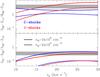 |
Fig. 10 Comparison of selected p-H2O line intensity ratios observed with PACS and shock model predictions from Flower & Pineau Des Forêts (2010). Red and blue curves represent J-type and C-type shock models respectively. The pre-shock gas density is n0 = 2 × 105 cm-3 (continuous curves) and n0 = 2 × 104 cm-3 (dotted curves). Low opacity lines from high energy rotational levels (Eu/k ~ 300−650 K) observed at similar wavelengths are selected. The upper panel shows the p-H2O 322–211/606–515 line ratio (89.988/83.284 μm) and the lower panel shows the 431–322/422–313 (56.325/57.637 μm) line ratios. The grey horizontal areas show the observed ratios and their error margins. |
Planar-shock model predictions of absolute H2O line intensities depend again on the unknown beam filling factor of the shocked material. Figure 10 shows a comparison of selected H2O line intensity ratios with recent unidimensional models of non-dissociative C-type and J-type shocks (the latter for vs < 30 km s-1) by Flower & Pineau Des Forêts (2010). In order to avoid using optically thick line diagnostics, different beam dilutions and extinction corrections, we selected low opacity p-H2O lines arising from high energy levels (Eu/k ~ 300−650 K) observed at similar wavelengths. The upper panel shows the 322−211/606–515 line ratio (89.988/83.284 μm) and the lower panel shows the 431−322/422−313 (56.325/57.637 μm) line ratio. The grey horizontal areas show the observed line intensity ratios and their error margins. From this comparison we conclude that low-velocity, non-dissociative shocks (vs ≲ 20 km s-1) with a pre-shock density of n0 ≃ 2 × 105 cm-3 are needed to reproduce the observed ratios. Figure 10 favors small-scale non-dissociative J-shocks, although it is difficult to determine any possible contribution of C-type shocks in the frame of current shock models and lack of spectral/angular resolution at λ < 100 μm.
Besides, the very different shock velocities required by Ne+ versus H2O lines suggests that both emissions arise from different locations. This will be the case if the Ne+ emission arises from fast shocks within the jet itself, but the H2O (and H2) emission arises in lower velocity shocks along the inner walls of the outflow cavity. Finally, note that the similar excitation conditions in the hot and dense gas (P/k = n TK ≃ 8 × 10⁹ K cm-3), as well as the similar spatial distribution of the nearby CO J = 29−28 and p-H2O 322–211 lines shown in Fig. 4 suggests that the hot CO and the excited H2O lines arise in the same shock component.
The UV radiation field probed by the [C ii]158 μm line can also heat the gas along the outflow cavity walls (see e.g., Visser et al. 2012). UV photons will modify the chemistry of the shocked gas (e.g., by photodissociating H2O and enhancing the OH and O abundances; see Sect. 5.3), but in terms of gas heating, they are likely not a dominant heating mechanism of the hot gas emission seen towards low-mass protostars (see Karska et al. 2012). All in all, the relative line intensities of the detected atomic and molecular species confirm the presence of both fast dissociative and lower velocity, non-dissociative shocks that are irradiated by UV radiation fields.
5.2. Line cooling
Complete far-IR and submm spectral scans allow an unbiased determination of the line cooling in YSOs. Line photons following collisional excitation and escaping the region are responsible of the gas cooling. Hence, the observed line luminosities in a broadband spectral scan provide a good measurement of the total gas cooling budget (see Table 1). In Serpens SMM1, ~54% of the total line luminosity is due to 12CO lines, followed by H2O (~22% and L(H2O)/L(12CO) ≃ 0.4), [O i] (~12%) and OH (9%). The total far-IR and submm line luminosity LFIR SMM = L(12CO)+L(H2O)+L(O i)+L(OH)+L(13CO)+L(C+) is LFIR SMM ≃ 0.12 L⊙, and the ratio Lmol/Lbol between the molecular line luminosity, Lmol = L(12CO)+L(H2O)+L(OH), and the bolometric luminosity is ≃3.5 × 10⁻³, all consistent with the expected emission of a Class 0 source (see e.g., Giannini et al. 2001). Note that only if the extinction in the mid-IR is larger than AV ≃ 200, then the intrinsic luminosity of the observed H2 lines will be higher than those of CO and H2O.
In our model, CO dominates the line cooling (Table 1) with more than half of the total CO luminosity arising from the warm component (a mixture of shocks and UV-illuminated material) and with a warm/hot luminosity ratio of L(COw)/L(COh) ≃ 5. H2O is the second most important species, with a dominant contribution to the hot shocked gas cooling. Note that we predict that ≳80% of the H2O line luminosity is radiated in the 55 μm < λ < 200 μm range and only ~5% at shorter wavelengths (in agreement with the absence of strong H2O lines in the Spitzer observations).
[O i] and OH lines also contribute to the gas cooling. In particular, both the absolute OH luminosities and the observed [O i]63 μm/H2 0−0 S(1) ≫ 1 intensity ratio are too bright for non-dissociative C-shock models (Kaufman & Neufeld 1996; Flower & Pineau Des Forêts 2010). As noted before, a significant fraction of the [O i] and OH line emission likely contributes to the cooling behind a fast, dissociative J-type shock.
5.3. Shock and UV-driven chemistry
The plethora of atomic fine-structure lines and to a lesser extent, the relatively high OH/H2O ≲ 0.5 abundance ratio inferred in the warm+hot component, confirms the presence of strong dissociative shocks in the inner envelope. In addition, owing to efficient H2O photodissociation, an enhanced UV radiation field illuminating the shocked gas can produce a high OH/H2O abundance ratios (see Goicoechea et al. 2011, in the Orion Bar PDR). The UV radiation field near low-mass protostars (roughly a diluted <10 000 K blackbody) is thought to be dominated by Ly α photons (10.2 eV) arising from accreting material onto the star (Bergin et al. 2003) and from fast dissociative J-shocks (Hollenbach & McKee 1979) such as those inferred in Serpens SMM1 (Sect. 5.1.1). Ly α radiation can dissociate H2O (producing enhanced OH and O) but can not dissociate CO (~11.1 eV) nor ionize sulfur (10.4 eV) or carbon (11.3 eV) atoms. However, if significant C+ and H2 are present, the ion-neutral drift in C-type shocks would significantly enhance the CH+ formation rate compared to J-type shocks (see Falgarone et al. 2010, for the detection of CH+ J = 1−0 broad outflow wings in the shock associated with the DR 21 massive star forming region). The lack of CH+ J = 3−2 emission in Serpens SMM1 provides an upper limit for the CH+ column density in the shocked gas (CH+/H2O < 0.01) and will help to constrain UV-irradiated shocks models (Kaufman et al., in prep.; Lesaffre et al., in prep.). The CH+ J = 3−2 line is detected in PDRs illuminated by massive OB stars where C+ is the dominant carbon species (Goicoechea et al. 2011; Nagy et al., in prep.) and, as in DR 21, the UV radiation field contains photons with energies higher than Ly α (up to 13.6 eV). Excited lines from reactive ions such as CO+ (that forms by reaction of C+ with OH) and are related with the presence of strong UV radiation fields in the shocked gas, are not detected in the PACS spectrum despite previous tentative assignations of several high-energy far-IR lines (see Ceccarelli et al. 1997, for IRAS 16293-2422)
The spatial distribution of the [C ii]158 μm line emission detected towards Serpens SMM1 (Fig. 4) is similar to that of other species in the outflow (with brighter emission in the outflow position than towards the protostar itself). The detection of faint C+ emission indicates the presence of a relatively weak UV field (but able to ionize C atoms and dissociate CO) along the outflow. Besides, the increase of the HCO+/HCN abundance ratio in the warm temperature component (HCN is easily photodissociated while HCO+ is abundant in the dense gas directly exposed to strong UV radiation) is another signature of UV photons. Indeed, the mere detection of [C i]370, 609 μm lines at the poor spectral resolution of the SPIRE-FTS towards the protostar shows that [C i] lines are significantly brighter than towards HH46 (van Kempen et al. 2009) or NGC 1333 IRAS 4A/4B (Yıldız et al. 2012). The presence of weak C+ line emission and of Ly α radiation in protostars like Serpens SMM1 (although difficult to detect) suggests that UV-irradiated shocks are a common phenomenon in YSOs.
X-ray emission is also expected in low-mass YSOs (Stäuber et al. 2006, 2007; Feigelson 2010) and they produce internally generated UV radiation fields after collisions of energetic photoelectrons with H and H2 (Maloney et al. 1996; Hollenbach & Gorti 2009). Although X-ray detections with Chandra have been reported towards the nearby Serpens SMM5, SMM6 and S68Nb protostars (Winston et al. 2007), the strength of any X-ray emission from Serpens SMM1 is unknown, possibly because of the high column density to the embedded source.
High sensitivity and velocity-resolved observations of CH+, CO+, SO+ and other reactive ions related with the presence of ionized atoms (e.g., C+ and S+) will help us to characterize these UV-irradiated shocks in more detail.
5.4. Comparison with other low-mass protostars
Comparative spectroscopy of protostars in different stages of evolution allows us to identify the common and the more peculiar processes associated with the first stages of star formation. Comparing the far-IR spectrum of the NGC 1333 IRAS 4B outflow to that of the Serpens SMM1 protostar, both show similar high H2O luminosities (L(H2O) ~ 0.03 L⊙). However, Serpens SMM1 shows a factor ~50 stronger [O i] luminosity and a lower L(H2O)/L(CO) ratio. The weak [O i] emission and high H2O luminosity in IRAS 4B outflow (L(H2O)/L(CO) ≃ 1) has been interpreted as non-dissociative C-shocks shielded from UV radiation (Herczeg et al. 2012). Indeed, C+ is not detected in IRAS 4B outflow whereas it is detected in Serpens SMM1 protostar and outflow (see Fig. 4). On the other hand, the strong [O i] and OH emission towards the Serpens SMM1 protostar itself is more similar to that of Class I source HH46 (van Kempen et al. 2010) where a L(OH)/L(H2O) ≃ 0.5 luminosity ratio has been inferred (vs. ~0.4 in SMM1). One possibility is that a high-velocity jet impinging on the dense inner envelope produces dissociative J-shocks (van Kempen et al. 2010) and enhanced [O i] and OH emission compared to non-dissociative C-shocks. Although they could not distinguish the dominant scenario, either J-shocks or UV-irradiated C-shocks have been also proposed to explain the OH emission seen in the high-mass YSO W3 IRS 5 (Wampfler et al. 2011).
The detection of [Ne ii], [Fe ii], [Si ii] and [S i] fine-structure lines towards Serpens SMM1 reinforces the scenario of both fast and slow shocks as well as UV radiation near the protostar, however, it is difficult to extract the exact geometry of the different shock components in the circumstellar environment (e.g., Ne+ versus H2O line emitting regions). Note that the presence of an embedded jet in the Class 0 source L1448 was reported from the detection of [Fe ii] and [Si ii] lines by Dionatos et al. (2009), and the same lines have been detected towards the nearby YSOs Serpens SMM3 and SMM4 (Lahuis et al. 2010). However, they did not detect the [Ne ii]12.8 μm line that requires fast shock velocities (Lahuis et al. 2007; Baldovin-Saavedra et al. 2012) or X-ray radiation (see Güdel et al. 2010, for Class II disk sources).
Compared to HH46, CO lines with Ju > 30 and higher excitation H2O lines are detected in Serpens SMM1 (not necessarily due to different excitation conditions but maybe just because lines are much brighter in SMM1). We have proposed that this hot CO and H2O emission arises from low velocity, non-dissociative shocks in the inner walls of the outflow cavity compressing the gas to very high thermal pressures (P/k = n TK ≃ 109−10 K cm-3). Based on the large gas compression factors and H2O line profiles seen toward several shock spots in bipolar outflows (far from the protostellar sources) Santangelo et al. (2012) and Tafalla et al. (in prep.) conclude that current low velocity J-shocks models explain their observations better than stationary C-shocks models. New shock models with a more detailed geometrical description and including the effects of UV radiation are clearly needed to determine the exact nature of the shocks inferred in the dense circumstellar gas near protostars.
The warm CO line emission (15 ≲ Ju ≲ 25) observed in Serpens SMM1 is a common feature in the far-IR spectrum of most protostars even if they are in different stages of evolution. This was previously observed by ISO (e.g., Giannini et al. 2001) and now by Herschel (e.g., Karska et al., submitted.; Green et al., in prep.; Manoj et al., in prep.). This CO emission ubiquity necessarily means that a broad combination of shock velocities and densities can produce a similar warm CO spectrum in different low- and high-mass YSOs.
The L(OH)/L(H2O), L(CO)/L([O i]) and L(H2O)/L([O i]) luminosity ratios in Serpens SMM1 have intermediate values between those in NGC 1333 IRAS 4B Class 0 YSO and HH46 Class I YSO (with ratios closer to SMM1) suggesting that the different luminosity ratios in IRAS 4B outflow are either a consequence of an earlier stage of evolution, or simply because the IRAS 4B outflow is peculiar, with very high H2O abundances not affected by UV photodissociation. Indeed, one of the main conclusions of all these studies is that water vapour lines are a roboust probe of shocked gas in protostellar environments. In Serpens SMM1 we infer a total H2Oh/(COh+COw) ≃ 0.02 abundance ratio in the warm+hot components traced by our far-IR observations. Only if the hot component was an independent physical component, the H2O abundances would be much higher (H2Oh/COh ≃ 0.4). However, this value is higher than the typical H2O/CO abundance ratios inferred from HIFI observations of the ground-state o-H2O 110–101 line (at ~557 GHz) towards a large sample of low-mass protostars (Kristensen et al. 2012). In these velocity-resolved observations, the H2O/CO abundance ratio increases from ~10-3 at low outflow velocities (<5 km s-1) to ~0.1 at high outflow velocities (>10 km s-1). Therefore, our inferred abundance ratio of H2Oh/(COh+COw) ≃ 0.02 from PACS observations seems a better description of the water vapour abundance in the protostellar shocked gas. Besides, it is also consistent with recent determinations from velocity-resolved HIFI observations of moderately excited H2O lines (Eu/k < 215 K) (see e.g., Santangelo et al. 2012, for L1448 outflow).
6. Summary and conclusions
We have presented the first complete far-IR and submm spectrum of a Class 0 protostar (Serpens SMM1) taken with Herschel in the ~55−671 μm window. The data are complemented with mid-IR spectra in the ~10−37 μm window retrieved from the Spitzer archive and first discussed here. These spectroscopic observations span almost 2 decades in wavelength and allow us to unveil the most important heating and chemical processes associated with the first evolutionary stages of low-mass protostars. In particular, we obtained the following results:
-
Serpens SMM1 shows a very rich far-IR andsubmm emission spectrum, with more than 145 lines, most ofthem rotationally excited lines of 12CO (up toJ = 42−41), H2O, OH, 13CO, HCN, HCO+and weaker emission from [C ii]158 and[C i]370, 609 μm.[O i]63 μm is the brightest line.Approximately half of the total far-IR and submm line luminosityis provided by CO rotational emission, withimportant contribution from H2O (~22%), [O i](~12%) and OH (~9%).
-
The mid-IR spectrum shows many fewer lines (probably due to severe dust extinction and lack of spectral resolution). Bright fine structure lines from Ne+, Fe+, Si+, and S, as well as weak H2 S(1) and S(2) pure rotational lines are detected.
-
The 12CO rotational diagram suggests the presence of 3 temperature components with T
 ≃
620 ± 30 K, T
≃
620 ± 30 K, T
 ≃ 340 ± 40 K
and T
≃ 340 ± 40 K
and T
 ≃ 100 ± 15 K.
As predicted by SED models in the literature, the detection of H2O, OH,
HCO+ and HCN emission lines from very high critical density transitions
suggests that the density in the inner envelope is high
(n(H2) ≳ 5 × 106 cm-3), and
thus the CO rotational temperatures provide a good approximation to the gas
temperature (Trot ≲ Tk).
≃ 100 ± 15 K.
As predicted by SED models in the literature, the detection of H2O, OH,
HCO+ and HCN emission lines from very high critical density transitions
suggests that the density in the inner envelope is high
(n(H2) ≳ 5 × 106 cm-3), and
thus the CO rotational temperatures provide a good approximation to the gas
temperature (Trot ≲ Tk).
-
A non-LTE, multi-component model allowed us to approximately quantify the contribution of the different temperature components (T
 ≈
800 K, T
≈
800 K, T
 ≈
375 K and
≈
375 K and
 ≈
150 K) and to estimate relative chemical abundances. The detected mid-IR
H2 lines provide a lower limit to H2 column density of
NH2 ≥ 1022 cm-2. We
derive the following upper limit abundances with respect to H2 in the
hot+warm components:
x(CO) ≤ 10-4, x(H2O) ≤
0.5 × 10⁻⁵ and x(OH) ≤ 10-6. The inferred
water vapour abundance is higher than the value typically found in cold interstellar
clouds but lower than that expected in hot shocked gas completely shielded from
UV radiation.
≈
150 K) and to estimate relative chemical abundances. The detected mid-IR
H2 lines provide a lower limit to H2 column density of
NH2 ≥ 1022 cm-2. We
derive the following upper limit abundances with respect to H2 in the
hot+warm components:
x(CO) ≤ 10-4, x(H2O) ≤
0.5 × 10⁻⁵ and x(OH) ≤ 10-6. The inferred
water vapour abundance is higher than the value typically found in cold interstellar
clouds but lower than that expected in hot shocked gas completely shielded from
UV radiation. -
Excited CO, H2O and OH emission lines arising from high energy levels are detected (up to Eu/k = 4971 K, Eu/k = 1036 K and Eu/k = 618 K respectively). These species arise in the hot+warm gas (M ≲ 0.03 M⊙) that we associate with a mixture of shocks. The observed hot CO, H2O and H2 lines provide a lower limit to the gas temperature of ~ 700 K. The excited H2O line emission is consistent with detailed model predictions of low-velocity non-dissociative shocks (with vs ≲ 20km s-1).
-
Fast dissociative (and ionizing) shocks with velocities vs > 60 km s-1 and pre-shock densities ≥ 104 cm-3 related with the presence of an embedded atomic jet are needed to explain the observed Ne+, Fe+, Si+ and S fine-structure emission and also the bright and velocity-shifted [O i]63 μm line emission. Dissociative J-shocks produced by the jet impacting the ambient material are the most probable origin of the bright [O i] and OH emission and of a significant fraction of the warm CO emission. In addition, water vapour photodissociation in UV-irradiated non-dissociative shocks along the outflow cavity walls can also contribute to the [O i] and OH emission.
Compared to other protostars, the large number of lines detected towards Serpens SMM1 reveals the great complexity of the protostellar environment. Both fast and slow shocks are needed to explain the presence of atomic fine structure lines and high excitation molecular lines. The spectra also show the signature of UV radiation (C+ and C towards the protostar and outflow). Therefore, most species (including H2O, OH, O and trace molecules such as CH+) arise in shocked gas illuminated by UV (even X-ray) radiation fields. Irradiated shocks are likely a very common phenomenon in YSOs.
Online material
Appendix A: Complementary figures and tables
List of detected lines towards Serpens SMM1 and line fluxes from SPIRE and PACS central spaxels (corrected for extended emission in the case of PACS).
continued.
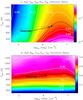 |
Fig. A.1 Grid of H2O LVG models for different gas temperatures and densities. Bottom: contour levels of the p-H2O 606–515/515–404 (83.284/95.627 μm) line ratio for N(p-H2O) = 1016 cm-2. Note the gas temperature dependence of this ratio. The black continuous curve shows the observed intensity line ratio of 0.33. Top: contour levels of the o-H2O 330–303/615–305 (67.269/82.031 μm) ratio for N(o-H2O) = 3 × 1016 cm-2. Note the gas density dependence of this ratio. The black continuous curve shows the observed intensity line ratio of 0.14 while the black dotted curve shows the observed p-H2O 606–515/515–404 ratio. The intersection of both curves is marked with a star (see text). |
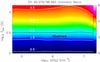 |
Fig. A.2 Grid of OH LVG models for different gas temperatures and densities. Contour
levels of the OH |

Mid-IR lines detected with Spitzer/IRS towards the Class 0 protostar Serpens SMM1 and line fluxes (uncorrected for extinction) within a 7′′ × 7′′ aperture.
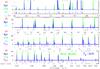 |
Fig. A.3 Best model discussed in the text (green curves) and a model where Tk is decreased by 30% in all components (blue curves). |
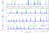 |
Fig. A.4 Best model discussed in the text (green curves) and a model where n(H2) is decreased by a factor 3 in all components (blue curves). |
Acknowledgments
We acknowledge our WISH internal referees, D. Neufeld and P. Bjerkeli for very helpful comments on an earlier version of the manuscript. We also thank the entire WISH team for many useful and vivid discussions in the last years. We finally thank the anonymous referee and M. Walmsley for useful comments. WISH research in Leiden is supported by the Netherlands Research School for Astronomy (NOVA), by a Spinoza grant and grant 614.001.008 from the Netherlands Organisation for Scientific Research (NWO), and by EU-FP7 grant 238258 (LASSIE). J.R.C., J.C. and M.E. thank the Spanish MINECO for funding support through grants AYA2009-07304 and CSD2009-00038. J.R.G. is supported by a Ramón y Cajal research contract from the MINECO and co-financed by the European Social Fund.
References
- Bachiller, R., & Tafalla, M. 1999, in The Origin of Stars and Planetary Systems, eds. C. J. Lada, & N. D. Kylafis, NATO ASIC Proc., 540, 227 [Google Scholar]
- Baldovin-Saavedra, C., Audard, M., Carmona, A., et al. 2012, A&A, 543, A30 [NASA ADS] [CrossRef] [EDP Sciences] [Google Scholar]
- Bergin, E., Calvet, N., D’Alessio, P., & Herczeg, G. J. 2003, ApJ, 591, L159 [NASA ADS] [CrossRef] [Google Scholar]
- Bontemps, S., Andre, P., Terebey, S., & Cabrit, S. 1996, A&A, 311, 858 [NASA ADS] [Google Scholar]
- Caselli, P., Keto, E., Pagani, L., et al. 2010, A&A, 521, L29 [NASA ADS] [CrossRef] [EDP Sciences] [Google Scholar]
- Ceccarelli, C., Caux, E., Wolfire, M., et al. 1997, in The first ISO workshop on Analytical Spectroscopy, eds. A. M. Heras, K. Leech, N. R. Trams, & M. Perry, ESA SP, 419, 43 [Google Scholar]
- Cernicharo, J. 2012, in Proc. of the European Conference on Laboratory Astrophysics, eds. C. Stehlé, C. Joblin, & L. d’Hendecourt, Eur. Astron. Soc. Publ. Ser., 2012, 4 [Google Scholar]
- Cernicharo, J., Goicoechea, J. R., Daniel, F., et al. 2006, ApJ, 649, L33 [NASA ADS] [CrossRef] [Google Scholar]
- Chiar, J. E., Ennico, K., Pendleton, Y. J., et al. 2007, ApJ, 666, L73 [NASA ADS] [CrossRef] [Google Scholar]
- Davis, C. J., Matthews, H. E., Ray, T. P., Dent, W. R. F., & Richer, J. S. 1999, MNRAS, 309, 141 [NASA ADS] [CrossRef] [Google Scholar]
- Dionatos, O., Nisini, B., Garcia Lopez, R., et al. 2009, ApJ, 692, 1 [NASA ADS] [CrossRef] [Google Scholar]
- Dionatos, O., Nisini, B., Codella, C., & Giannini, T. 2010, A&A, 523, A29 [NASA ADS] [CrossRef] [EDP Sciences] [Google Scholar]
- Draine, B. T., & McKee, C. F. 1993, ARA&A, 31, 373 [NASA ADS] [CrossRef] [Google Scholar]
- Dzib, S., Loinard, L., Mioduszewski, A. J., et al. 2010, ApJ, 718, 610 [NASA ADS] [CrossRef] [Google Scholar]
- Eiroa, C., Djupvik, A. A., & Casali, M. M. 2008, The Serpens Molecular Cloud, ed. B. Reipurth, 693 [Google Scholar]
- Enoch, M. L., Corder, S., Dunham, M. M., & Duchêne, G. 2009, ApJ, 707, 103 [NASA ADS] [CrossRef] [Google Scholar]
- Evans, II, N. J., Dunham, M. M., Jørgensen, J. K., et al. 2009, ApJS, 181, 321 [NASA ADS] [CrossRef] [Google Scholar]
- Falgarone, E., Ossenkopf, V., Gerin, M., et al. 2010, A&A, 518, L118 [NASA ADS] [CrossRef] [EDP Sciences] [Google Scholar]
- Feigelson, E. D. 2010, Proc. National Academy of Science, 107, 7153 [Google Scholar]
- Flower, D. R., & Pineau Des Forêts, G. 2010, MNRAS, 406, 1745 [NASA ADS] [Google Scholar]
- Giannini, T., Nisini, B., & Lorenzetti, D. 2001, ApJ, 555, 40 [NASA ADS] [CrossRef] [Google Scholar]
- Goicoechea, J. R., & Cernicharo, J. 2002, ApJ, 576, L77 [NASA ADS] [CrossRef] [Google Scholar]
- Goicoechea, J. R., Cernicharo, J., Lerate, M. R., et al. 2006, ApJ, 641, L49 [NASA ADS] [CrossRef] [Google Scholar]
- Goicoechea, J. R., Joblin, C., Contursi, A., et al. 2011, A&A, 530, L16 [NASA ADS] [CrossRef] [EDP Sciences] [Google Scholar]
- Griffin, M. J., Abergel, A., Abreu, A., et al. 2010, A&A, 518, L3 [Google Scholar]
- Güdel, M., Lahuis, F., Briggs, K. R., et al. 2010, A&A, 519, A113 [NASA ADS] [CrossRef] [EDP Sciences] [Google Scholar]
- Herczeg, G. J., Karska, A., Bruderer, S., et al. 2012, A&A, 540, A84 [NASA ADS] [CrossRef] [EDP Sciences] [Google Scholar]
- Hogerheijde, M. R., van Dishoeck, E. F., Salverda, J. M., & Blake, G. A. 1999, ApJ, 513, 350 [NASA ADS] [CrossRef] [PubMed] [Google Scholar]
- Hollenbach, D., & Gorti, U. 2009, ApJ, 703, 1203 [NASA ADS] [CrossRef] [Google Scholar]
- Hollenbach, D., & McKee, C. F. 1979, ApJS, 41, 555 [NASA ADS] [CrossRef] [Google Scholar]
- Hollenbach, D., & McKee, C. F. 1989, ApJ, 342, 306 [NASA ADS] [CrossRef] [Google Scholar]
- Houck, J. R., Roellig, T. L., van Cleve, J., et al. 2004, ApJS, 154, 18 [NASA ADS] [CrossRef] [Google Scholar]
- Karska, A., Herczeg, G. J., van Dishoeck, E. F., et al. 2012, A&A, submitted [Google Scholar]
- Kaufman, M. J., & Neufeld, D. A. 1996, ApJ, 456, 611 [NASA ADS] [CrossRef] [Google Scholar]
- Kristensen, L. E., van Dishoeck, E. F., Bergin, E. A., et al. 2012, A&A, 542, A8 [NASA ADS] [CrossRef] [EDP Sciences] [Google Scholar]
- Lahuis, F., van Dishoeck, E. F., Blake, G. A., et al. 2007, ApJ, 665, 492 [NASA ADS] [CrossRef] [Google Scholar]
- Lahuis, F., van Dishoeck, E. F., Jørgensen, J. K., Blake, G. A., & Evans, N. J. 2010, A&A, 519, A3 [NASA ADS] [CrossRef] [EDP Sciences] [Google Scholar]
- Langer, W. D., & Penzias, A. A. 1990, ApJ, 357, 477 [NASA ADS] [CrossRef] [Google Scholar]
- Laor, A., & Draine, B. T. 1993, ApJ, 402, 441 [NASA ADS] [CrossRef] [Google Scholar]
- Larsson, B., Liseau, R., Men’shchikov, A. B., et al. 2000, A&A, 363, 253 [NASA ADS] [Google Scholar]
- Larsson, B., Liseau, R., & Men’shchikov, A. B. 2002, A&A, 386, 1055 [NASA ADS] [CrossRef] [EDP Sciences] [Google Scholar]
- Maloney, P. R., Hollenbach, D. J., & Tielens, A. G. G. M. 1996, ApJ, 466, 561 [NASA ADS] [CrossRef] [Google Scholar]
- Melnick, G. J., Tolls, V., Neufeld, D. A., et al. 2008, ApJ, 683, 876 [NASA ADS] [CrossRef] [Google Scholar]
- Neufeld, D. A., & Dalgarno, A. 1989, ApJ, 340, 869 [NASA ADS] [CrossRef] [Google Scholar]
- Neufeld, D. A., Melnick, G. J., Sonnentrucker, P., et al. 2006, ApJ, 649, 816 [NASA ADS] [CrossRef] [Google Scholar]
- Nisini, B., Bacciotti, F., Giannini, T., et al. 2005, A&A, 441, 159 [NASA ADS] [CrossRef] [EDP Sciences] [Google Scholar]
- Offer, A. R., & van Dishoeck, E. F. 1992, MNRAS, 257, 377 [NASA ADS] [Google Scholar]
- Pilbratt, G. L., Riedinger, J. R., Passvogel, T., et al. 2010, A&A, 518, L1 [CrossRef] [EDP Sciences] [Google Scholar]
- Poglitsch, A., Waelkens, C., Geis, N., et al. 2010, A&A, 518, L2 [NASA ADS] [CrossRef] [EDP Sciences] [Google Scholar]
- Rodríguez, L. F., Loinard, L., D’Alessio, P., Wilner, D. J., & Ho, P. T. P. 2005, ApJ, 621, L133 [NASA ADS] [CrossRef] [Google Scholar]
- Santangelo, G., Nisini, B., Giannini, T., et al. 2012, A&A, 538, A45 [NASA ADS] [CrossRef] [EDP Sciences] [Google Scholar]
- Smith, J. D. T., Armus, L., Dale, D. A., et al. 2007, PASP, 119, 1133 [NASA ADS] [CrossRef] [Google Scholar]
- Stäuber, P., Jørgensen, J. K., van Dishoeck, E. F., Doty, S. D., & Benz, A. O. 2006, A&A, 453, 555 [NASA ADS] [CrossRef] [EDP Sciences] [Google Scholar]
- Stäuber, P., Benz, A. O., Jørgensen, J. K., et al. 2007, A&A, 466, 977 [NASA ADS] [CrossRef] [EDP Sciences] [Google Scholar]
- van Dishoeck, E. F., Kristensen, L. E., Benz, A. O., et al. 2011, PASP, 123, 138 [NASA ADS] [CrossRef] [Google Scholar]
- van Kempen, T. A., van Dishoeck, E. F., Hogerheijde, M. R., & Güsten, R. 2009, A&A, 508, 259 [Google Scholar]
- van Kempen, T. A., Kristensen, L. E., Herczeg, G. J., et al. 2010, A&A, 518, L121 [NASA ADS] [CrossRef] [EDP Sciences] [Google Scholar]
- Visser, R., Kristensen, L. E., Bruderer, S., et al. 2012, A&A, 537, A55 [NASA ADS] [CrossRef] [EDP Sciences] [Google Scholar]
- Walmsley, M., Pineau des Forêts, G., & Flower, D. 2005, in Astrochemistry: Recent Successes and Current Challenges, eds. D. C. Lis, G. A. Blake, & E. Herbst, IAU Symp., 231, 135 [Google Scholar]
- Wampfler, S. F., Bruderer, S., Kristensen, L. E., et al. 2011, A&A, 531, L16 [NASA ADS] [CrossRef] [EDP Sciences] [Google Scholar]
- Wampfler, S. F., Bruderer, S., Karska, A., et al. 2012, A&A, submitted [Google Scholar]
- Watson, D. M., Bohac, C. J., Hull, C., et al. 2007, Nature, 448, 1026 [NASA ADS] [CrossRef] [PubMed] [Google Scholar]
- Whittet, D. C. B. 2003, Dust in the galactic environment [Google Scholar]
- Winston, E., Megeath, S. T., Wolk, S. J., et al. 2007, ApJ, 669, 493 [NASA ADS] [CrossRef] [Google Scholar]
- Yıldız, U. A., Kristensen, L. E., van Dishoeck, E. F., et al. 2012, A&A, 542, A86 [NASA ADS] [CrossRef] [EDP Sciences] [Google Scholar]
All Tables
List of detected lines towards Serpens SMM1 and line fluxes from SPIRE and PACS central spaxels (corrected for extended emission in the case of PACS).
Mid-IR lines detected with Spitzer/IRS towards the Class 0 protostar Serpens SMM1 and line fluxes (uncorrected for extinction) within a 7′′ × 7′′ aperture.
All Figures
|
Fig. 1 PACS and SPIRE (lower panel) continuum-subtracted spectra of Serpens SMM1 (central spaxel) with H2O (blue), CO (red), OH (cyan), 13CO (magenta), [O i], [C ii] and [C i] (green), and HCO+ and HCN (black) lines labelled. The flux density scale is in Jy (assuming a point source). |
| In the text | |
|
Fig. 2 Observed spectral energy distribution (SED) of Serpens SMM1 and modified blackbody fit (red curve). Inset shows the full PACS array in flux density units of 10-14 W m-2 μm-1. The abscissa is in linear scale from 55 to 190 μm. The bright emission line seen in several positions is [O i]63 μm. Approximate outflow directions are shown with red and blue arrows. |
| In the text | |
|
Fig. 3 Upper: SPIRE-FTS 12CO J = 9−8 and 12−11 sparse maps. Lower: p-H2O 111–000 and 202–111 maps respectively. The line surface brightness is on the 10-8 W m-2 sr-1 scale. The white contours represent the 50% line emission peak level. The FWHM beam is shown in each inset. Note the increase of line surface brightness in the more excited lines. |
| In the text | |
|
Fig. 4 PACS spectral maps of Serpens SMM1 in the o-H2O
303–212 (174.626 μm);
[C ii]157.741 μm; CO J = 17−16
(153.267 μm); both
p-H2O 322–211
(89.988 μm) and CO J = 29−28
(90.163 μm); [O i]63.183 μm and OH
|
| In the text | |
|
Fig. 5 a) Spitzer IRS spectrum of the Class 0 protostar Serpens SMM1 using the Hi Res modules and a 7′′ × 7′′ aperture. b) Continuum-subtracted spectra with main narrow lines identified in the LH module (λ ≥ 19.5 μm) and c) with the SH module (λ ≤ 19.5 μm). Note the lack of bright molecular line emission (H2O, OH, etc.). |
| In the text | |
|
Fig. 6 12CO and 13CO rotational diagrams obtained from PACS and SPIRE spectra. The estimated error in Trot for 12CO corresponds to different choices of Ju cutoffs for the different components. The range of possible Trot for 13CO reflects the standard error on the fitted values. |
| In the text | |
|
Fig. 7 H2O rotational diagram showing o-H2O (filled circles) and p-H2O far-IR lines (open circles). Owing to subthermal excitation (Trot ≪ Tk) and large opacities of most lines, the H2O diagram displays a larger scatter (standard error on the fitted values are shown) than CO. |
| In the text | |
|
Fig. 8 Synthetic non-LTE LVG spectrum of the Class 0 protostar Serpens MM1 convolved to PACS (top three panels) and SPIRE (lower panel) spectral resolutions. Continuous curves show the line emission contribution from the “hot” (red), “warm” (green) and “cool” (blue) components discussed in the text. Vertical labels mark the wavelength position of CO (red), H2O (blue), OH (cyan), 13CO (magenta), HCO+ and HCN (grey) rotational transitions. [O i]63, 145 and [C i]370, 609 μm fine structure lines are marked with green labels. |
| In the text | |
|
Fig. 9 Herschel far-IR and submm spectrum of Serpens SMM1 at the central spaxel position (black histogram) and complete model (green continuous curves) adding the emission from the hot, warm and cool components and convolved to PACS and SPIRE spectral resolutions. |
| In the text | |
|
Fig. 10 Comparison of selected p-H2O line intensity ratios observed with PACS and shock model predictions from Flower & Pineau Des Forêts (2010). Red and blue curves represent J-type and C-type shock models respectively. The pre-shock gas density is n0 = 2 × 105 cm-3 (continuous curves) and n0 = 2 × 104 cm-3 (dotted curves). Low opacity lines from high energy rotational levels (Eu/k ~ 300−650 K) observed at similar wavelengths are selected. The upper panel shows the p-H2O 322–211/606–515 line ratio (89.988/83.284 μm) and the lower panel shows the 431–322/422–313 (56.325/57.637 μm) line ratios. The grey horizontal areas show the observed ratios and their error margins. |
| In the text | |
|
Fig. A.1 Grid of H2O LVG models for different gas temperatures and densities. Bottom: contour levels of the p-H2O 606–515/515–404 (83.284/95.627 μm) line ratio for N(p-H2O) = 1016 cm-2. Note the gas temperature dependence of this ratio. The black continuous curve shows the observed intensity line ratio of 0.33. Top: contour levels of the o-H2O 330–303/615–305 (67.269/82.031 μm) ratio for N(o-H2O) = 3 × 1016 cm-2. Note the gas density dependence of this ratio. The black continuous curve shows the observed intensity line ratio of 0.14 while the black dotted curve shows the observed p-H2O 606–515/515–404 ratio. The intersection of both curves is marked with a star (see text). |
| In the text | |
|
Fig. A.2 Grid of OH LVG models for different gas temperatures and densities. Contour
levels of the OH |
| In the text | |
|
Fig. A.3 Best model discussed in the text (green curves) and a model where Tk is decreased by 30% in all components (blue curves). |
| In the text | |
|
Fig. A.4 Best model discussed in the text (green curves) and a model where n(H2) is decreased by a factor 3 in all components (blue curves). |
| In the text | |
Current usage metrics show cumulative count of Article Views (full-text article views including HTML views, PDF and ePub downloads, according to the available data) and Abstracts Views on Vision4Press platform.
Data correspond to usage on the plateform after 2015. The current usage metrics is available 48-96 hours after online publication and is updated daily on week days.
Initial download of the metrics may take a while.