| Issue |
A&A
Volume 547, November 2012
|
|
|---|---|---|
| Article Number | A93 | |
| Number of page(s) | 11 | |
| Section | The Sun | |
| DOI | https://doi.org/10.1051/0004-6361/201219833 | |
| Published online | 06 November 2012 | |
Basal magnetic flux and the local solar dynamo
1
Institute of Astronomy,
ETH Zurich,
8093
Zurich,
Switzerland
e-mail: This email address is being protected from spambots. You need JavaScript enabled to view it.
2
Istituto Ricerche Solari Locarno, via Patocchi,
6605
Locarno Monti,
Switzerland
Received: 18 June 2012
Accepted: 27 September 2012
Abstract
The average unsigned magnetic flux density in magnetograms of the quiet Sun is generally dominated by instrumental noise. Due to the entirely different scaling behavior of the noise and the solar magnetic pattern it has been possible to determine the standard deviation of the Gaussian noise distribution and remove the noise contribution from the average unsigned flux density for the whole 15-yr SOHO/MDI data set and for a selection of SDO/HMI magnetograms. There is a very close correlation between the MDI disk-averaged unsigned vertical flux density and the sunspot number, and regression analysis gives a residual level of 2.7 G when the sunspot number is zero. The selected set of HMI magnetograms, which spans the most quiet phase of solar activity, has a lower limit of 3.0 G to the noise-corrected average flux density. These apparently cycle-independent levels may be identified as a basal flux density, which represents an upper limit to the possible flux contribution from a local dynamo, but not evidence for its existence. The 3.0 G HMI level, when scaled to the Hinode spatial resolution, translates to 3.5 G, which means that the much higher average flux densities always found by Hinode in quiet regions do not originate from a local dynamo. The contributions to the average unsigned flux density come almost exclusively from the extended wings of the probability density function, also in the case of HMI magnetograms with only basal-level magnetic flux. These wings represent intermittent magnetic flux. As the global dynamo continually feeds flux into the small scales at a fast rate through turbulent shredding, a hypothetical local dynamo may only be relevant to the Sun if its rate of flux build-up can be competitive. While the global dynamo appears to dominate the magnetic energy spectrum at all the resolved spatial scales, there are indications from the observed Hanle depolarization in atomic lines that the local dynamo may dominate the spectrum at scales of order 1−10 km and below.
Key words: Sun: atmosphere / magnetic fields / polarization / dynamo / magnetohydrodynamics (MHD)
© ESO, 2012
1. Introduction
Dynamo processes are responsible for the generation of macroscopic magnetic fields from feeble seed fields (Larmor 1919; Elsasser 1946, 1956). The solar dynamo, which is the source of the 11-year activity cycle with its sunspots, flares, CMEs, prominences, etc., is a prototype of a cosmic dynamo. The basic ingredients of the Sun’s dynamo are the same as for the galactic and planetary dynamos: interactions between magnetic fields and turbulence in an electrically conducting and rotating medium. The rotation breaks the left-right symmetry of the turbulence through the Coriolis force, thereby generating a large-scale net helicity that is the source of the dynamo-produced magnetic field (Parker 1955; Steenbeck & Krause 1969).
While the symmetry breaking mechanism can produce magnetic patterns on large scales, turbulent shredding ensures that the magnetic scale spectrum extends over many orders of magnitudes, down to the magnetic diffusion limit near 10−100 m, far below the observationally resolved scales on the Sun (cf. Stenflo 2012). The magnetic energy that is injected at large scales by the dynamo quickly cascades all the way down the scale spectrum. The turbulent scale redistribution of the globally generated magnetic energy gives the Sun’s magnetic field a fractal-like appearance.
In the context of numerical simulations of magneto-convection the concept of a small-scale, “local dynamo” that operates near the solar surface has often been used to account for much of the small-scale magnetic structuring (Kazantsev 1968; Petrovay & Szakaly 1993; Cattaneo 1999; Brandenburg & Subramanian 2005). In contrast to the previously discussed “global dynamo”, the local dynamo does not need a rotating medium or the breaking of the left-right symmetry of the convective motions but simply depends on the way convection tangles the magnetic field. However, in the great majority of the numerical simulations done to date, the amount of magnetic energy that is generated at small scales depends on the initial conditions of the simulation, and therefore they do not represent any local dynamo.
A local dynamo only exists in the simulations if, without input from any global dynamo, magnetic energy can be built up from an initial seed field, and if the results of the simulations are independent of the choice of seed field. One clear demonstration that such a local dynamo is possible on the Sun is that of Vögler & Schüssler (2007), but, as the authors point out, their results depend on chosen simulation idealizations, like the subgrid model for the viscosity. Therefore this demonstration cannot be interpreted as proving that a local dynamo contributes significantly to the observed small-scale magnetic fields on the real Sun.
The question how relevant a local dynamo is for the Sun cannot be determined by numerical simulations alone, because their results depend on the idealizations and simplifications that have to be introduced. Instead we have to look for empirical answers derived from the observed properties of the Sun, trying to separate the relative contributions from the global and local dynamos.
We know that the cyclic behavior of the Sun’s magnetic field (22-yr magnetic cycle with the 11-yr sunspot cycle) is the result of global dynamo action. In contrast the local dynamo is related to the quiet Sun and produces magnetic fields that are statistically time invariant. Therefore a local dynamo can only contribute to a possible “basal flux”, a minimum magnetic flux level that is always present everywhere and every time on the Sun, even in the complete absence of sunspots and solar activity. The observed presence of a basal X-ray flux for slow-rotating cool stars (Schrijver 1987) has been interpreted as empirical evidence for the existence of dynamo action in non-rotating plasmas without symmetry breaking from the Coriolis effect (Bercik et al. 2005).
In the next sections we will use data from SOHO/MDI (Scherrer et al. 1995) and SDO/HMI (Scherrer et al. 2012; Schou et al. 2012) to determine the Sun’s basal magnetic flux density level. Since the apparent, time-invariant flux level has its main contribution from instrumental noise, we have developed a technique to statistically separate the noise and solar contributions from each other, to find the noise-free, intrinsic basal flux level. Such a separation is possible because the noise and the solar field obey completely different scaling laws. The basal flux density level is resolution dependent, but in a way that is well defined from a known scaling law. The low value of the determined basal flux density allows us to place a tight limit to the possible contribution of a local dynamo to the observed small-scale magnetic fields on the Sun.
2. Correlation between unsigned flux and sunspot number
Recently a global analysis of the complete set of 96 min cadence SOHO/MDI full disk magnetograms, 73 838 of them covering the 15-yr period May 1996−April 2011, was carried out with the aim of exploring the properties of bipolar magnetic regions (Stenflo & Kosovichev 2012). As a byproduct of this analysis we determined for each magnetogram the average value Bave of the unsigned vertical flux density |Bv| over a circular region around disk center, for which the normalized radius vector r/r⊙ was less than 0.1, 0.2, ..., 0.8, and 0.9, respectively, including all pixels in the average (regardless of whether they occur in sunspots or not). This allows us to explore how well the value of Bave correlates with the sunspot number for the various sizes of the averaging regions.
The vertical flux density Bv was obtained from the line-of-sight component B∥ of the magnetograms through the simple relation Bv = B∥/μ, where μ is the cosine of the heliocentric angle of the respective pixel in the image. This procedure is based on the assumption that the fields are on average oriented in the vertical direction. While this is the only practically feasible assumption that can be made, it is physically justified (at least for statistical purposes outside active regions) by the circumstance that most (>90%) of the net flux recorded with the MDI 4 arcsec resolution comes from collapsed, kG type flux elements (Howard & Stenflo 1972; Stenflo 1973, 1994). Such strong fields get pushed in the vertical direction by the buoyancy forces in the photospheric layers where the fields are measured. Higher (above the observed layers) the field starts to become force-free and may increasingly deviate from the vertical. Errors due to this assumption will contribute to statistical scatter. The circumstance that the relation between the disk averaged flux density and the sunspot number turns out to be so tight, as we will see next, lends support to this procedure.
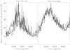 |
Fig. 1 Time series of the average of the unsigned vertical flux density, smoothed with a 1-month wide time window (solid lines). Left panel: averaging over the disk region r/r⊙ < 0.1. Right panel: averaging over the disk region r/r⊙ < 0.9. The dashed curves use a second-order polynomial in the sunspot number (also smoothed with a 1-month time window) to fit the solid curves. The fit gets tighter as the disk averaging area increases. |
Figure 1 shows as the solid curves the value of Bave, time smoothed with a 1-month wide window, for two choices of the averaging region: r/r⊙ < 0.1 (left panel), and r/r⊙ < 0.9 (right panel). The dashed curves represent the monthly averages of the international sunspot number Rz, converted to a magnetic field scale BRz through the second-order relation  (1)This relation is fitted to the solid curves with the coefficients as the three free fit parameters, which gives us the dashed curves.
We see from Fig. 1 that the disk-averaged value of |Bv| (right panel) can be nearly perfectly modeled, the fit is surprisingly tight, implying that there is an almost one-to-one relation between Bave and the sunspot number. If we however only use the innermost portion of the solar disk for the averaging of |Bv| (left panel), then Bave fluctuates rather wildly, in particular during times of high solar activity, and the fit with the sunspot number is poor. The reason is of course that the magnetic field in the disk center region is not representative of the overall level of magnetic activity on the Sun. The presence or absence of individual low-latitude active regions govern the behavior of |Bv| near disk center. One needs to account for the cumulative magnetic contributions over a large portion of the disk to get a good representation of solar activity.
It is nevertheless surprising that the sunspot number Rz turns out to be such a nearly perfect index for the overall magnetic activity of the Sun as represented by the disk average of the unsigned vertical flux density. The largest deviations between the model fit and the data in the right panel of Fig. 1 occur in regions of significant data gaps in the MDI time series (1998.48−1998.89 and 1998.97−1999.17), so the physically relevant fit is even better than it may appear in the plot. As the size of the averaging region is increased, the fit between the Rz model and Bave becomes quite tight already for r/r⊙ < 0.5, and the fit improves only slowly as we go to still larger averaging areas. For r/r⊙ < 0.9 (right panel of Fig. 1) the fit parameters of the model have the values (in G) b0 = 19.0, b1 = 0.24, and b2 = −5.5 × 10⁻⁴.
Coefficient b0, as defined by Eq. (1), can be interpreted as representing the apparent basal flux density, the minimum level reached in the absence of sunspots. However, instrumental noise contributes to a fictitious non-zero basal level, since the noise does not average out to zero when we average over the absolute, unsigned flux densities. Recently a careful noise analysis of the MDI magnetograms by Liu et al. (2012) showed that the instrumental noise is indeed of the same order as our apparent basal flux density level of 19 G. This indicates that the intrinsic level of the basal flux density must be much smaller. A determination of its actual value requires a very careful separation and removal of the noise contribution. The procedure for doing this is described in the next section.
3. Statistical removal of MDI noise
Fortunately it is possible to statistically separate the noise contribution from the intrinsic solar contribution, since the Gaussian noise and the fractal-like solar magnetic pattern obey entirely different scaling laws. The two contributions however combine in a way that is neither linear nor quadratic. Before we can model the scaling behavior we need to determine the form of the non-linear relation between the noise-affected and noise-free average unsigned flux densities, which will be done in the next subsection.
3.1. Convolution of noise with the intrinsic PDF
Let P(Bv) be the area normalized probability density function (PDF) for the intrinsic, noise-free flux densities. Then the average unsigned flux density is  (2)As shown in a detailed analysis of Hinode SOT/SP data for the quiet Sun disk center (Stenflo 2010), P(Bv) is characterized by an extremely narrow core peak centered at Bv = 0, which can be modeled by a stretched exponential. This peak is surrounded by quadratically declining damping wings that extend out to the kG region. The contribution to Bave is completely dominated by the contribution from the damping wings, since the inner PDF core is so narrow.
The apparent, noise-affected PDF, Papp, is obtained from the intrinsic P through direct convolution with the noise distribution, which can safely be assumed to have a Gaussian shape. For a Gaussian distribution with standard deviation σ, the average of the unsigned field value of the distribution is 0.798σ. If the intrinsic PDF were also Gaussian, then the convolved distribution would remain Gaussian with a sigma that is obtained by adding the two individual sigmas quadratically. In contrast, when convolving two Lorentzian profiles (which have quadratically declining wings, like the solar PDFs), their half widths add linearly. In the present case, however, we are convolving a Gaussian with a function that is more Lorentzian like. We would therefore expect that the average unsigned field values would combine in a way that is neither quadratic nor linear, but somewhere in between. In the following we will determine the form of this relation.
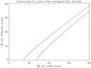 |
Fig. 2 Relation between the noise-free average unsigned vertical flux density (vertical axis, in the text denoted Bave) and the corresponding noise-affected flux density (horizontal axis, in the text denoted Bapp), for two values of σ for the noise distribution, 18 and 34 G. The solid curves are obtained through numerical convolution of PDFs that are representative of quiet-sun magnetic fields (as derived from Hinode analysis) with Gaussian noise distributions, while the dashed curves are analytical representations of the solid curves in terms of Eqs. (3) and (4). |
The noise-affected average unsigned flux density Bapp, which is obtained from Eq. (2) if we replace P by Papp, can be determined directly from any given value for the noise σ by direct numerical Gaussian convolution of P. To obtain this relation also as a function of Bave, representing solar regions with varying amount of magnetic flux, we have used the analytical shape of the symmetrized intrinsic PDF that represented our Hinode disk center data set (Stenflo 2010), and produced a family of P(Bv) distributions by varying the value of the damping parameter that governs the strength of the damping wings of the PDF and therefore also the value of Bave. The result of these numerical convolutions and integrations are shown by the solid curves in Fig. 2, computed for two chosen values of the noise σ, 18 and 34 G. Note that the average unsigned field values for these two Gaussians are smaller than these sigmas by the factor 0.798 and are thus 14.4 and 27.1 G, respectively.
Next we have replaced the Hinode-type shape of P with a Lorentzian function and repeated the calculations. Convolution of a Lorentzian function with a Gaussian gives the well-known Voigt function. The resulting curves are practically indistinguishable from the solid curves in Fig. 2 and are therefore not plotted. This result is not unexpected, since the non-Lorentzian core of the Hinode PDF P does not contribute significantly to the value of Bave, and the PDF wings have the same shape as a Lorentzian function. Therefore our modeling is insensitive to the true shape of the PDF core region.
As we will later use inversion techniques to determine the actual noise in the magnetograms and calculate the scaling law for the noise-affected flux density, we need to represent the numerical results in Fig. 2 (the solid curves) in an analytical form, valid for arbitrary choices of the noise σ. Based on the considerations that we have made before about the way in which Gaussian and Lorentzian functions combine, our analytical model for the conversion of the noise-affected Bapp to the noise-free Bave for a given value of the standard deviation σ of the noise distribution is ![Mathematical equation: \begin{equation} B_{\rm ave} =[\,B_{\rm app}^\alpha\,-\,(0.798\sigma)^\alpha\,]^{(1/\alpha)}. \label{eq:noisemod} \end{equation}](/articles/aa/full_html/2012/11/aa19833-12/aa19833-12-eq31.png) (3)For two Gaussian functions α would be 2.0, for two Lorentzian functions it would be 1.0. By choosing α (through trial and error) to be
(3)For two Gaussian functions α would be 2.0, for two Lorentzian functions it would be 1.0. By choosing α (through trial and error) to be  (4)we obtain the dashed curves in Fig. 2, which can be seen to be nearly perfect representations of the exact, numerical relations. More importantly, our analytical model remains an excellent representation not just for the two chosen sigmas of the two curves in Fig. 2, but for arbitrary values of σ across the range spanned by these two σ values. This is the range within which we will find the actual MDI noise values to lie.
We note in Eq. (4) that α falls between the values 2 and 1 for the Gaussian and Lorentzian cases, as expected.
3.2. Scaling law for the average unsigned flux density
The unsigned vertical flux density is a resolution dependent quantity because the pattern of solar magnetic fields contains mixed magnetic polarities across the whole range of spatial scales (resolved and unresolved). Due to cancellation of the positive and negative contributions of the opposite-polartiy magnetic fluxes within each resolution element, the net flux or apparent flux density (as averaged over the resolution element) is reduced. As we increase the spatial resolution more of the mixed polarity elements get resolved, which reduces the cancellation effects. This causes the average of the unsigned vertical flux density to increase.
The scaling law that governs the variation of the average unsigned vertical flux density is called the cancellation function. It was introduced by Pietarila Graham et al. (2009) for analysis of a Hinode SOT/SP data set for the quiet Sun disk center, which had been converted to vertical flux densities by Lites et al. (2008). The cancellation function  (5)describes how the average unsigned flux density Bave for a given region on the Sun depends on the chosen resolution scale d. Through numerical smoothing of the Hinode data Pietarila Graham et al. (2009) determined the value of the cancellation exponent κ to be 0.26. The determination is however sensitive to the influence of instrumental noise and the way in which the polarimetric data are converted to flux densities. An independent determination of the cancellation exponent from quiet-sun Hinode data led to κ = 0.13, a value half as large (Stenflo 2011). If, as it seems, the pattern of solar magnetic fields behaves like a fractal, we expect κ to be independent of scale size d over several orders of magnitude, including scales larger than the MDI resolution and unresolved small scales beyond the Hinode resolution.
Random instrumental noise, which is spatially uncorrelated from pixel to pixel, scales with 1/ , where N is the number of pixels inside the smoothing window (simulated resolution element), implying a κ of unity, representing a much steeper scaling law than that of the magnetic-field pattern. Noise has the effect of spuriously steepening the cancellation function.
The 96 min cadence SOHO/MDI data set of full disk magnetograms that we have used contains a mixture of magnetograms based on two distinctly different integration times, 1 min and 5 min. A keyword in the fits file header identifies which integration time was used for the given magnetogram. Since the noise characteristics are distinctly different for the two choices of integration time, we have divided the entire data set into two subsets, each representing the respective integration time.
In their recent analysis of the noise in the MDI magnetograms, Liu et al. (2012) estimated the disk-averaged value for the standard deviation σ of the noise distribution to be 16.2 and 26.4 G for the magnetograms with 5-min and 1-min integrations, respectively. They considered these values to only be upper limits, since they had been obtained by fitting Gaussians to the PDF cores in quiet solar regions, assuming that the solar contribution to the core width can be neglected. If this assumption is incorrect, the actual noise is smaller.
The values of Liu et al. (2012) are for the disk-averaged line-of-sight component B∥, while our analysis is based on the vertical flux density Bv = B∥/μ within radius vector r/r⊙ < 0.9. Since the average of 1/μ within this radius vector is 1.39, we should multiply by this factor to translate the Liu et al. values to a scale that is comparable to ours. Their values then become 22.5 and 36.7 G. Note however that this crude translation only represents an estimate, because the noise is not constant over the disk but has a large-scale pattern. Nevertheless it serves as a reference to check the consistency of the analysis. As we will see in the next subsection, our use of the scaling laws to determine the noise σ leads to the values 18.8 and 33.2 G, which are 10−20% smaller than the corresponding values of Liu et al. (2012). As their results represent upper limits, our results are fully consistent with theirs.
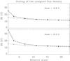 |
Fig. 3 Average unsigned vertical flux density vs. relative size (in pixel units) of the smoothing window, illustrated for two representative magnetograms, one obtained with 5-min integration (upper panel), the other with 1-min integration (lower panel). The solid curves represent the observed, noise-affected values Bapp, the dotted curves the noise-free values Bave, while the dashed curves are obtained through combination of Bave with the noise σ according to the model described by Eqs. (3) and (4). |
In Fig. 3 we illustrate for two representative magnetograms how the two scaling laws, with κ = 1 for the noise and κ = 0.13 for the magnetic fields, combine to give a scaling behavior that can be fitted to the observational data. The average unsigned vertical flux density over r/r⊙ < 0.9 is plotted as a function of the relative scale d, in units of the MDI pixel size. d represents the side of the square-shaped window used for numerical spatial smoothing. The solid curves are the actually observed values Bapp of the average unsigned flux density, the dotted curves the inferred intrinsic average unsigned flux density Bave, while the dashed curves represent the modeled combination of Bave with a noise σ (for d = 1) of 18.8 G (upper panel) and 33.2 G (lower panel). We see that the agreement between the model (dashed) and observations (solid) is nearly perfect in both cases. It is through fitting of the model to the observations that the noise σ is determined, as will be described next. This determination also leads to a verification that κ = 0.13 is indeed the correct cancellation exponent to use.
3.3. Determination of the noise levels
For the model fitting to determine the noise contribution to the observed average unsigned flux densities Bapp we have randomly selected 320 MDI magnetograms evenly distributed over the 15 yr period of MDI operation. The fits header keywords reveal that 140 of these magnetograms represent recordings with 5-min integration, 180 with 1-min integration. The magnetograms have then been spatially smoothed with square windows having side d = 3, 7, 11, 15, 19, and 23 pixels. For each magnetogram there are thus 7 versions with different degrees of smoothing. They are all converted to vertical flux densities Bv through division by μ for each pixel. |Bv| is then averaged over the disk region r/r⊙ < 0.9 to give the noise-affected average unsigned vertical flux density Bapp as a function of d. For each magnetogram we thus obtain 7 observables (which in Fig. 3 are represented by the filled circles and solid lines, for the choice of two magnetograms).
These 7 observables serve as input for an iterative least squares model fitting. The fit model is based in Eqs. (3)−(5), with the Bapp values for the 7 different d values being the observables to be fit. For convenience we introduce the notation Bsolar to refer to the value of Bave for the unsmoothed case (to distinguish it from the more general notation Bave, which may refer to any smoothed case and therefore depends on d). Then the d-independent model parameters to be determined are Bsolar, σ, and cancellation exponent κ. For reasons of numerical robustness we only let Bsolar and σ be free model parameters, while keeping the value of κ fixed, but repeat the fit procedure for a sequence of κ values to demonstrate that only one particular value of κ leads to physically acceptable results.
Let us here mention the technical detail that Bsolar, the unsmoothed version of Bave, actually refers to d = 2, since according to the sampling theorem there must be at least 2 × 2 pixels per resolution element. Therefore the resolution does not increase when we go from d = 2 to d = 1. In contrast, the sampling theorem does not apply to the noise, which does not contain spatial structures. In Fig. 3 we have plotted the value of Bsolar at d = 1 (as the left ends of the dotted lines), because it relates to the values of Bapp and σ at d = 1. The practical consequences of the sampling theorem are however insignificant, since the solar scaling is so small when going from d = 1 to 2. Thus 2κ is only 1.09 for κ = 0.13.
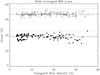 |
Fig. 4 Standard deviation σ of the Gaussian noise distribution (vertical axis) vs. noise-free average unsigned vertical flux density, determined from least-squares fits to the randomly selected 320 MDI magnetograms, assuming a cancellation exponent κ = 0.13. The filled circles have been obtained from magnetograms recorded with 5-min integration, the open circles from magnetograms with 1-min integration. The solid horizontal lines at 18.8 and 33.2 G represent the average values of σ for the two populations. For comparison the corresponding upper limits to the noise levels as derived from the analysis of Liu et al. (2012) are given as the dotted lines. |
Our least squares fitting gives us for each of the 320 magnetograms the two determined fit parameters Bsolar and σ, the standard deviation of the Gaussian noise distribution. In Fig. 4 we have for a cancellation exponent κ = 0.13 plotted σ as a function of Bsolar, using filled circles for the magnetograms that were obtained with 5-min integrations, open circles for the magnetograms based on 1-min integrations. We see that the filled and open circles form two distinctly different populations, as expected. The two horizontal lines mark the average values of σ for each population, 18.8 and 33.2 G, respectively. For comparison we give as the dotted lines the upper limits to σ, 22.5 and 36.7 G, derived by Liu et al. (2012) but here scaled with the average value of 1/μ inside r/r⊙ < 0.9 to make them refer to our vertical flux density scale. They lie 10−20% higher than our solid lines, which is fully consistent with the circumstance that they represent upper limits only.
The two magnetograms that we selected for illustration of the scaling behavior in Fig. 3 were chosen to have Bsolar values in the middle of the range spanned by the 320 magnetograms. Thus the Bsolar value for the upper panel is 15.6 G, for the lower panel 15.2 G. The corresponding points in Fig. 4 lie almost exactly on the horizontal lines that represent the average σ for the respective point population.
It is gratifying that there is no dependence of the fitted value of the noise σ on the magnetic flux level Bsolar of a given magnetogram. Any such dependence would be unphysical if the noise is of instrumental origin and is fully stochastic and additive, like photon noise, and since the brightness-flux correlation is very small when recorded with 4 arcsec resolution (except in sunspots, which are expected to only have a minor influence on the global flux averages). However, this flux invariance of σ turns out to be unique for the chosen value of cancellation exponent κ. For other values of κ the point distribution in Bsolar − σ space is tilted. We have repeated the fitting procedure for a sequence of fixed κ values, determined the slopes of the regression line fits to the point populations, and plotted these slopes with their error bars as a function of κ in Fig. 5. The filled circles and solid line represent the magnetograms with 5-min exposure, the open circles and dashed line the magnetograms with 1-min exposure. We see that both sets of magnetograms give zero slope only for κ = 0.13, while for all other choices of κ an unphysical non-zero slope is found. It is this result that unambiguously leads us to the unique value κ = 0.13.
The same value of κ was found from an analysis of the scaling behavior of Hinode magnetograms for the quiet-sun disk center (Stenflo 2011). This consistency between the widely different Hinode and MDI data provides support for the validity of our noise model, while indicating that κ is indeed invariant over a large scale range, as expected from fractal-like behavior of the magnetic field pattern. The circumstance that the same noise model with the same κ, when applied to the quite different HMI data set for the quiet-sun disk center, also gives a noise σ that does not depend on the magnitude of the unsigned flux density (cf. Fig. 7), further supports the validity of our approach.
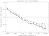 |
Fig. 5 Regression line slopes with error bars for the point populations in diagrams of the type of Fig. 4, based on model fitting with different fixed values for the cancellation exponent κ. The filled circles and solid line represent magnetograms with 5-min integration, while the open circles and dashed line represent magnetograms with 1-min integration. Only zero slope is physically acceptable, which occurs when κ = 0.13 (marked by the vertical dotted line). |
3.4. Noise-corrected correlation with the sunspot number
Having determined the two values of the noise σ for the 5-min and 1-min exposure magnetograms, we can now apply Eqs. (3) and (4) to convert the noise-affected average unsigned vertical flux density Bapp to its noise-free counterpart Bave. Similar to the right panel of Fig. 1 we plot as the solid curve in Fig. 6 Bave for the set of 5-min exposure magnetograms, time-smoothed with a 1-month window. Like in Fig. 1 we model this curve in terms of a second-order polynomial in the sunspot number Rz (also time-smoothed with a 1-month window), defined by Eq. (1). The resulting values for the fit parameters in units of G are: b0 = 2.7, b1 = 0.25, and b2 = −5.0 × 10⁻⁴. Except for the value of b0 (Bave in the absence of sunspots) the fit parameters (b1 and b2) are nearly identical to those of Fig. 1. For b0, however, there is a dramatic change, from 19.0 G in the noise-affected case to 2.7 G in the noise-free case. The noise-corrected value of b0 may be interpreted as a time-invariant, basal flux density of the Sun.
The corresponding time series of the noise-corrected Bave based on the use of the 1-min exposure magnetograms is nearly identical although somewhat noisier and is therefore not illustrated separately here. The polynomial fit parameters are slightly different: b0 = 1.0, b1 = 0.28, and b2 = −6.5 × 10⁻⁴. This difference gives an indication of the uncertainty in the determination of the basal flux level. As the noise σ for the 1-min magnetograms is almost twice as large (33.2 G) as for the 5-min magnetograms (18.8 G), we give considerably more weight to the analysis based on these lower-noise magnetograms. As we will see below, our 2.7 G level found with the 5-min MDI magnetograms is fully consistent with the 3.0 G level that we find from analysis of SDO/HMI magnetograms. The consistency between the MDI and HMI results supports the conclusion that the basal flux density of about 3 G is a real physical property of the Sun.
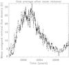 |
Fig. 6 Time series of the noise-corrected disk average (over the disk region r/r⊙ < 0.9) of the unsigned vertical flux density, smoothed with a 1-month wide time window (solid line). Due to an MDI data gap the solid line is absent in the interval 1998.4−1999.0. The dashed curve uses a second-order polynomial in the sunspot number (also smoothed with a 1-month time window) to fit the solid curve. This polynomial fit gives a basal flux density (in the absence of sunspots) of 2.7 G. |
4. Basal flux density from HMI data
The Helioseismic and Magnetic Imager (HMI) on the Solar Dynamics Observatory (SDO; Scherrer et al. 2012; Schou et al. 2012) is the next-generation successor of the MDI instrument on SOHO and has been operating since April 2010. HMI delivers line-of-sight magnetograms with a cadence of 45 s and a spatial resolution that is four times higher than that of MDI, with a noise level that is better than that of the 5-min MDI magnetograms by more than a factor of 2. This substantial improvement in quality makes the HMI data particularly suited for a determination of the basal flux density level.
The advantage of the MDI data set over that of HMI is that the MDI time series of 15 yr covers more than a full sunspot cycle, which allows an exploration of the correlation between disk-averaged unsigned flux density and sunspot number, as we have done in Figs. 1 and 6. The second-order polynomial fit to the sunspot number allowed us to identify the constant coefficient in the polynomial fit as the basal value of the disk-averaged vertical flux density, since it represents the flux density in the absence of sunspots. This type of approach is not possible with the HMI data, since HMI so far only covers a small fraction of a solar cycle.
The HMI data set on the other hand has the advantage of covering in great detail a cycle phase when the Sun has been unusually quiet. During this phase the average unsigned flux densities should come closest to the minimum level that is given by the basal flux density.
Like with the MDI data, the apparent basal flux density of the HMI data is dominated by the noise contribution. A determination of the basal flux density therefore has to be preceded by an accurate modeling and determination of the HMI noise. This is done in the following subsection.
4.1. HMI noise at disk center
For our HMI analysis we have selected 676 magnetograms, one for each day, starting April 30, 2010. The procedure for the determination of the standard deviation σ of the Gaussian noise distribution with least squares model fitting based on the different scaling behavior of the noise and the magnetic fields is identical to the procedure that we used for MDI and which was described in great detail in Sect. 3.3. For each HMI magnetogram we thus generate 7 different versions with different degrees of spatial smoothing. However, since we are not doing correlations with the sunspot number, there is no reason for averaging the unsigned flux density over most of the solar disk. Instead we only do the averaging over the central portion of the disk, within r/r⊙ < 0.1. Inside this disk-center region there is no significant difference between the vertical and the line-of-sight directions, so no geometrical projection is needed to convert the line-of-sight component to a vertical component. With our previous notations, Bapp is the apparent, noise-affected average unsigned vertical flux density within r/r⊙ < 0.1, while Bave is its noise-free counterpart. Like for MDI, Eqs. (3)−(5), with cancellation exponent κ = 0.13, are applicable also for HMI, since these equations are not resolution dependent over the spatial scales that we are considering.
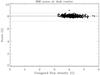 |
Fig. 7 Standard deviation σ of the Gaussian noise distribution (vertical axis) vs. noise-free average unsigned vertical flux density, determined from least-squares fits to the disk-center regions of a set of HMI magnetograms, based on the same fitting procedure as used for Fig. 4. The average σ (solid horizontal line) is found to be 8.0 G. For comparison we give as the dotted horizontal lines the upper and lower limits to the HMI disk center noise σ, as determined by Liu et al. (2012). |
The results of the least squares parameter fitting are shown in Fig. 7, where the noise σ is plotted vs. Bsolar, the value of the noise-corrected Bave for the unsmoothed version of the magnetogram. The average value of σ, marked by the horizontal solid line, is found to be 8.0 G. For comparison we draw as the horizontal dotted lines the upper and lower limits to the HMI noise as derived from the careful analysis by Liu et al. (2012). The upper limit of 8.5 G was obtained by Gaussian fitting to the core region of the observed PDF in quiet regions, while the lower limit of 7.2 G represents the ideal, theoretically expected level based on Monte Carlo simulations of the photon noise in HMI. The perfect consistency of our results with these two limits strongly supports the validity of our noise model based on the use of scaling laws.
Note that the HMI σ of 8.0 G is small in comparison with the disk-averaged σ of 18.8 and 33.2 G for the 5-min and 1-min MDI magnetograms. Therefore the domination of the noise contribution relative to the solar basal flux contribution will be much less severe for HMI as compared with the MDI data set.
4.2. Basal flux density from the noise-corrected HMI time series
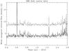 |
Fig. 8 Time series (2010.4–2011.6) of the noise-affected average unsigned vertical flux density (dashed curve) and its counterpart after noise removal (solid curve), representing the disk center region (r/r⊙ < 0.1). The solid curve never dips below the 3.0 G level, which can be interpreted as the basal flux density at the HMI resolution of 1 arcsec. |
With the determined value of σ = 8.0 G we can now, exactly like we did in Sect. 3.4 for the MDI data, use Eqs. (3) and (4) to convert the noise-affected average unsigned vertical flux density Bapp to its noise-free counterpart Bsolar (which represents Bave for the unsmoothed magnetograms). Since we have analyzed one HMI magnetogram per day, we get a time series, which we have plotted in Fig. 8 for the most quiet period of solar activity, from 2010.4 to 2011.6. The noise-corrected average flux density Bsolar is plotted as the solid curve, while the time series Bapp before noise removal is shown as the dashed curve for comparison.
While the value of the noise-free Bsolar can be seen to vary significantly from day to day, it never drops below the 3.0 G level marked by the dotted line, although the illustrated period represents an unusually deep and extended quiet phase of the solar activity cycle. The 3.0 G level may therefore be interpreted as the basal unsigned vertical flux density of the Sun, which is always present, regardless of the level of solar activity.
It is difficult to give a good estimate for the error bar in the 3.0 G HMI basal flux density level, since the error is most likely dominated by systematic effects (like the degree of validity of our noise model) rather than by formal fitting errors. In the case of the MDI analysis, the difference in the b0 values of 2.7 G for the 5-min integration magnetograms and 1.0 G for the 1-min integration magnetograms gives an indication of the degree of significance of the determination, although we give more weight to the 5-min magnetograms because they are less noisy to start with. Similarly, we give still more weight to the HMI analysis, due to the higher quality and much lower noise of the HMI data set, and since we only use disk center data with no reference to sunspots.
Still one may wonder if the HMI 3.0 G level could be much different, for instance close to zero, due to errors in our approach. This question will be clarified in the next section by comparing the appearance of a magnetogram that represents the basal flux level with one that has more than twice as much average flux density. If the basal flux density were much less than 3 G, then the “basal magnetogram” would look much more empty, with much less visibility of the magnetic network, and the flux density histograms for the two magnetograms would differ much more than they do. From such considerations we can exclude a basal flux density level below about 2 G.
The basal flux level is dependent on spatial resolution (but not on integration time, since the temporal evolution of the magnetograms within the integration times that we are dealing with is insignificant). The given values refer to the particular spatial resolution used (1 arcsec in the case of HMI) and scales with the resolution according to the law given by Eq. (5) with cancellation exponent κ = 0.13. The HMI 3.0 G level therefore translates to 3.0 × 4-0.13 = 2.5 G for the 4 arcsec MDI resolution. This scaling is in nearly perfect agreement with the value of 2.7 G that we determined from the analysis of the 5-min MDI magnetograms through the correlation between the unsigned vertical flux density and the sunspot number over the solar cycle. In the next section we will discuss the physical meaning of this result.
5. Basal flux and the local dynamo
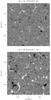 |
Fig. 9 Comparison of the disk-center portions (| x|, |y| < 0.1 r⊙) of two HMI magnetograms, recorded at times 2011.2086 (upper panel) and 2011.4796 (lower panel), when the average of the unsigned vertical flux density was 3.06 and 6.65 G, respectively. The upper panel thus represents the case when the basal flux density level is approximately reached. The grey-scale cuts are at ± 50 G in both panels. |
While the average unsigned flux density is a convenient parameter to characterize the statistical properties of the magnetic pattern in terms of a single number, we need to examine the full pattern to understand what this number really means. For this purpose we illustrate in Fig. 9 the disk-center regions of two HMI magnetograms, both representing the quiet Sun, but with different values of Bsolar, the noise-corrected average unsigned vertical flux density. For the upper panel, Bsolar = 3.06 G, nearly identical with our estimate of the basal flux density level, while for the lower panel it is 6.65 G, significantly larger although still quite small. The plotted regions extend in x (E-W direction) and y (S-N direction) over ± 0.1 r⊙ with respect to disk center. The grey scale cuts in both plots are −50 G (dark) and + 50 G (white). The upper and lower magnetograms are from times 2011.2086 and 2011.4796, respectively, and can be identified in the time series of Fig. 8 as a local dip and a local peak at these times.
While the two magnetograms are qualitatively similar, in both cases characterized by a magnetic network on the scale of the supergranulation, they are strikingly different quantitatively, as expected from the difference of more than a factor of two of their Bsolar values. Note that before noise correction the apparent average unsigned flux densities were 8.1 and 10.8 G and therefore did not differ that much from each other (since these values are dominated by the noise contributions).
5.1. Intermittent basal magnetic flux
To make the comparison between the two magnetograms in Fig. 9 more explicit and quantitative, we plot in Fig. 10 the respective histograms of the vertical flux density, as the solid line for the upper magnetogram, as the dashed line for the lower one. These histograms (which we refer to as empirical PDF, without implying any assumption concerning the underlying physical process), contain the noise contribution, since the noise-removal procedure that we applied to the average unsigned flux densities can only be used for this statistical ensemble average. For comparison we have therefore in Fig. 10 plotted as the dotted curve the Gaussian noise distribution with the determined standard deviation σ of 8.0 G. It agrees almost perfectly in the PDF core region with the two solar PDFs, which only differ from it by their extended damping wings.
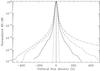 |
Fig. 10 Amplitude-normalized PDFs for the two magnetograms in Fig. 9 (solid line for the upper magnetogram, dashed line for the lower) and for the Gaussian noise distribution with σ = 8.0 G (dotted line). For comparison we have also plotted as the dash-dotted line the analytical representation of the PDF from the Hinode quiet-sun analysis of Stenflo (2010), after having convolved it with the σ = 8.0 G Gaussian to make it comparable to the HMI PDFs. |
The effect of noise on the observed PDF is a Gaussian convolution of the intrinsic, solar PDF. In principle one could therefore retrieve the noise-free solar PDF through deconvolution. The circumstance that the Gaussian noise profile almost perfectly matches the core regions of the solar PDFs means, however, that the core width of the solar PDF is insignificant in comparison with the noise broadening.
Through forward modeling with Hinode quiet-sun data from February 27, 2007, it was found that an analytical representation in terms of a stretched exponential for the core region, supplemented by extended, quadratically declining wings, gave an excellent representation of the observed PDF when convolved with the Gaussian noise distribution (Stenflo 2010). With this analytical PDF one finds that the average unsigned flux density is almost exclusively determined by the PDF damping wings, although the PDF core region represents the vast majority of the pixels (the dominating filling factor). In fact, if one changes the strength of the wings by decreasing the damping parameter in the analytical representation, the average unsigned flux density may go down to values even far below 1 G, but the exact value of the lower limit depends on the details of the not so well known intrinsic shape of the narrow core region.
It is thus the extended PDF wings that are the source of the determined (noise-free) values of the average unsigned flux density, including the value of the basal flux density. The solid-line PDF in Fig. 10 is representative of the magnetic pattern at the basal flux density level. The difference in wing amplitude between the dashed and solid PDFs is fully consistent with the conclusion that the wing region is the source of the difference between their intrinsic Bsolar values, 6.65 and 3.06 G. In contrast, the apparent Bapp values of 10.8 and 8.2 G are dominated by the contribution from the noise-dominated Gaussian PDF core.
For comparison with our HMI-based PDFs, we plot our analytical representation of the mentioned Hinode PDF, but only after it has been convolved with the Gaussian σ = 8.0 G PDF. This convolution is done exclusively for the purpose of allowing us to quantitatively compare the relative magnitudes of the different PDF wings on a common scale. This comparison reveals that the quiet region picked by Hinode contained significantly more magnetic flux than our two HMI regions. The different PDFs in Fig. 10 illustrate that there is a broad range of quiet-region flux levels, and that this variable quiet-sun flux can have nothing to do with a time invariant local dynamo. The qualitatively similar PDF shapes indicate that all of them are produced by the same type of physical processes, including the solid-line PDF that can be taken as representative of the basal flux level.
The extended PDF wings are a signature of intermittency, since the combination of high flux density with low occurrence probability in the PDF wings implies significant spatial separation between such relatively rare, strong-field elements. The circumstance that the dominant contribution to the unsigned average flux density always comes from the wings rather than from the PDF core implies that the magnetic flux is highly intermittent, including the basal flux. The intermittency expresses itself in Fig. 9 in the form of discrete flux fragments that form a network-like pattern.
It has been argued that while the PDF wings that represent the intermittent network-type flux may be asymmetric between the positive and negative polarities, the PDF core (defined to refer to the internetwork) is always symmetric, and that a symmetric, invariant PDF core is a signature of a local dynamo (Lites 2011). However, we have demonstrated here that when the noise contribution is removed from the PDF, the magnitude of the unsigned average flux density is almost entirely (beyond the 1 G level) determined by the intermittent PDF wings.
The apparent existence of a time invariant basal flux level may seem to point toward an origin in terms of a local dynamo. The flux generated by the global dynamo however spreads to form a background field pattern across the whole surface of the Sun, and this background does not suddenly vanish when the sunspot number goes to zero. The decay and removal of flux from the solar photosphere has a certain time scale, which becomes longer when the flux level decreases, because flux removal has to do with encounters between flux fragments of opposite polarities. Due to the extreme flux intermittency, the polarity encounters become increasingly rare as the flux density level goes down. Therefore the background flux does not have enough time to be fully removed before the next cycle injects new flux into the background.
This implies that the global dynamo will always leave a residual, non-zero flux density that will be indistinguishable from the basal flux density that we have determined. Therefore we can only say that our basal flux density represents an upper limit to the small-scale flux density that may hypothetically be generated by a local dynamo.
5.2. Hidden basal-type flux from the Hanle effect
It has long been known from applications of the Hanle effect that the solar photosphere is seething with a ubiquitous magnetic field that is tangled on scales much smaller than the telescope resolution and therefore does not show up in magnetograms that are based on the Zeeman effect (Stenflo 1982, 1987). The “Second Solar Spectrum”, the linearly polarized spectrum that is exclusively produced by coherent scattering processes and which is the playground for the Hanle effect became accessible to systematic exploration in 1994 (Stenflo & Keller 1996, 1997) through the introduction of the ZIMPOL technology for high-precision imaging polarimetry (Povel 1995, 2001; Gandorfer et al. 2004). From the series of observing campaigns with ZIMPOL since then we have been able to notice how the general appearance of the Second Solar Spectrum has changed with the solar cycle, from an “emission-like” spectrum (in Stokes Q/I) full of intrinsically polarizing lines during solar minimum, to a mixed emission- and absorption-like spectrum during the maximum phase (the period extensively documented in the Atlas of the Second Solar Spectrum, Gandorfer 2000). While the polarization of the molecular lines seemed to be nearly invariant with the cycle, the atomic lines exhibited large variations (Stenflo 2003). Another intriguing finding was that the turbulent field strength derived from the Hanle effect in molecular lines was much smaller than the value obtained from the Sr i 4607 Å line (Trujillo Bueno et al. 2004).
In 2007 a synoptic program was started with ZIMPOL at IRSOL (Istituto Ricerche Solari Locarno) to explore the solar-cycle variations of the small-scale, tangled magnetic field with the differential Hanle effect (Stenflo et al. 1998) in molecular C2 lines at 5141 Å. Assuming a single-valued field strength and an isotropic angular distribution, an average field of 7.4 ± 0.8 G was found for the period 2007−2009, with no evidence for a significant temporal evolution (Kleint et al. 2011). This field therefore appears to have the characteristics of a basal flux at the scale where the tangled field resides.
The value of 7.4 G seems to nicely relate to the 3.0 G basal level determined for the HMI spatial scale. Applying the d−κ scaling law with κ = 0.13, we find that 3.0 G becomes 7.4 G if we go down to the 0.7 km scale. This lies in the middle of the scale range for the hidden flux that was recently estimated (Stenflo 2012) based on an analysis of the magnetic energy spectrum of the quiet Sun over scales spanning 7 orders of magnitude. It was argued that the most logical location for the tangled hidden flux is just below the range of 10−100 km, where most of the kG type flux tubes reside. The tangled fields may exist all the way down to the magnetic diffusion limit around 10−100 m, but since their strength is expected to weaken as we go down in scale, their main contribution should come from the upper end of the range below a few km.
In contrast to this modest value for the basal hidden flux derived from the differential Hanle effect in the optically thin molecular C2 lines, the Hanle effect in atomic lines reveals a hidden field that is an order of magnitude stronger. The most elaborate modeling so far (Trujillo Bueno et al. 2004) of the Hanle depolarization observed in the Sr i 4607 Å line has led to a field strength of 60 G for the hidden field (assuming a single-valued PDF with an isotropic angular distribution). Trujillo Bueno et al. (2004) explain this difference in terms of a spatial correlation of the hidden flux with the solar granulation. Their modeling shows that the C2 lines are formed exclusively in the interior of the granulation cells, while the Sr line has contributions from both the intergranular lanes and cell interiors. The implication is that the hidden, tangled field is much stronger in the intergranular lanes than in the cell centers, which appears plausible, since the collapsed kG type flux also strongly correlates with the intergranular lanes (Stenflo 2011). The flux of the small-scale tangled field may therefore be supplied by the decaying flux tubes (Stenflo 2012).
This interpretation has got support from Snik et al. (2010), who could record scattering polarization in molecular CN lines with sufficient spatial resolution to allow a weak statistical distinction between the intergranular lanes and the cell interiors. More Hanle depolarization was found in the lanes, implying stronger fields there. Shapiro et al. (2011) did detailed Hanle-effect radiative transfer modeling of the ultraviolet CN lines and found them to give field strengths of similar large magnitudes as those found with the Sr i 4607 Å line. The circumstance that the molecular CN lines (and the Sr line) are optically thick, in contrast to the optically thin C2 lines, appears to be related to the difference in their behavior. To settle this issue we need high-resolution mapping of the Hanle depolarization effect in the Sr line, to determine if the field-strength contrast between the intergranular lanes and cell interiors really is as huge as the interpretation models indicate.
Unfortunately it is difficult to find suitable atomic line pairs for applications of the differential Hanle effect, in contrast to many good choices of molecular line pairs. Interpretation of the Hanle effect in atomic lines therefore depends more on absolute than differential polarimetry as well as on the details of the radiative-transfer modeling, including the 3D geometry of the atmosphere, the effects of the atomic collisions, and the small-scale thermodynamic structure. We need a differential approach to reduce this model dependence.
A controversial issue is also whether the strong (of order 60 G) hidden field revealed by the atomic lines varies with the solar cycle. The conspicuous change in the overall appearance of the atomic lines in the Second Solar Spectrum with the solar cycle is evidence for substantial cyclic variations of the hidden flux (Stenflo 2003). In contrast, Trujillo Bueno et al. (2004) have assembled some evidence from various observations of the Sr i 4607 Å line that the large field strength that they deduce from this line does not vary with the cycle. We need a synoptic program for the atomic lines to quantitatively settle this issue and determine how high the basal, time-invariant component of the hidden flux density really is.
6. Concluding remarks
The magnetic energy spectrum of the Sun extends over more than 7 orders of magnitude, from the global scales down to the magnetic diffusion scale around 10−100 m, where the magnetic field lines cease to be frozen-in and decouple from the plasma (Stenflo 2012). Apart from the scales in the range 10−100 km, where most of the intermittent flux tubes formed by the convective collapse mechanism are expected to reside, there is no particular preferred length scale in this magneto-convective spectrum, which could form a basis for deciding what is local and what is global. The spectrum extends all the way down to the magnetic diffusion limit, regardless of whether a local dynamo exists or not.
The global dynamo is a source of small-scale magnetic structuring, but it also needs the small scales for its operation. Much of the large-scale helicity is produced by the statistical left-right symmetry breaking in the ensemble of small-scale turbulent elements. The question whether a local dynamo is physically relevant for the Sun depends on whether the rate at which it can create new magnetic flux from a seed field is competitive with the rate at which magnetic flux is fed into the small scales by the turbulent shredding of flux that has been created by global dynamo processes.
Analysis of the observed magnetic flux in MDI and HMI magnetograms shows that there is an apparently time invariant average unsigned flux density of 3.0 G at the 1 arcsec spatial scale. This basal level represents an upper limit to the contribution of a hypothetical local dynamo. It corresponds to 3.5 G when scaled to the Hinode 0.3 arcsec scale with the cancellation function that we have empirically found to be valid over this scale range. Since the average unsigned flux densities found in quiet solar regions with Hinode are much larger, most of the quiet-sun magnetic flux that has been recorded with Hinode has nothing to do with a local dynamo.
The average unsigned flux densities are determined almost exclusively by the extended damping wings of the flux density PDFs, also in the 3.0 G case that represents the basal flux. The PDF wings are signatures of the intermittent nature of the field. A residual background flux level on the Sun (with a small number density of intermittent flux fragments) may survive over relatively long periods in the absence of solar activity and fresh input from the global dynamo. The 3.0 G level that we have found therefore does not necessarily imply a significant contribution from a local dynamo. An interesting question is what would happen to the basal-type background flux during a Maunder-type minimum. If there is a local dynamo, it should maintain a certain flux density level indefinitely, even if the global dynamo were to be turned off.
Analysis of the differential Hanle effect in optically thin molecular C2 lines indicates the existence of a time-invariant, basal-type field of strength 7.4 G, representing the region in the interior of granulation cells. Modeling of the Hanle effect observed in atomic lines (like the Sr i 4607 Å line) and the optically thick CN lines in the UV gives field strengths that are larger by an order of magnitude. This apparent contradiction may be explained if the hidden field is much stronger in the intergranular lanes than in the cell interiors. It remains controversial how much of the strong hidden flux represents time-invariant, basal flux. To clarify the nature of these fields we need to apply differential techniques and map the Hanle effect with a spatial resolution that resolves the solar granulation.
If much of the strong hidden flux (with strength of order 60 G or more) really represents a basal flux, then this large field strength cannot be directly connected via a fractal scaling law to the 3.0 G basal level that we have determined for the 1 arcsec spatial scale. While the 3 G value places a very tight upper limit to the possible contribution of a local dynamo to the spatially resolved fields, the 60 G value, if basal, offers plenty of room for a local dynamo. This leads us to a scenario, in which the relative contribution of the local dynamo is insignificant at all the scales that can be resolved by current instruments, but in which the local dynamo becomes the dominant agent at the smallest scales in the unresolved domain, probably around and below the 1−10 km scale (where the hidden flux is estimated to reside according to Stenflo 2012). The generation of magnetic energy by the local dynamo at these small scales would then raise the energy spectrum and flatten it in the domain that leads down to the magnetic diffusion limit. A synoptic differential Hanle observing program for photospheric atomic lines is needed to determine whether this scenario applies to the Sun.
Acknowledgments
I am grateful for the hospitality of Stanford University during a visit in March 2012 for work on the SDO/HMI and SOHO/MDI data sets, and for the help provided by Sasha Kosovichev to develop convenient IDL program access to the huge HMI and MDI data archives at Stanford. I also want to thank Yang Liu for helpful discussions about the noise characteristics of the MDI and HMI magnetograms, and Göran Scharmer for bringing my attention to the effect of noise on determinations of the basal flux density.
References
- Bercik, D. J., Fisher, G. H., Johns-Krull, C. M., & Abbett, W. P. 2005, ApJ, 631, 529 [NASA ADS] [CrossRef] [Google Scholar]
- Brandenburg, A., & Subramanian, K. 2005, Phys. Rep., 417, 1 [NASA ADS] [CrossRef] [Google Scholar]
- Cattaneo, F. 1999, ApJ, 515, L39 [NASA ADS] [CrossRef] [Google Scholar]
- Elsasser, W. M. 1946, Phys. Rev., 69, 106 [NASA ADS] [CrossRef] [MathSciNet] [Google Scholar]
- Elsasser, W. M. 1956, Rev. Mod. Phys., 28, 135 [NASA ADS] [CrossRef] [Google Scholar]
- Gandorfer, A. 2000, The Second Solar Spectrum: A high spectral resolution polarimetric survey of scattering polarization at the solar limb in graphical representation, Vol. I: 4625 Å to 6995 Å (Zurich: VdF) [Google Scholar]
- Gandorfer, A. M., Steiner, P., Povel, H. P., et al. 2004, A&A, 422, 703 [NASA ADS] [CrossRef] [EDP Sciences] [Google Scholar]
- Howard, R., & Stenflo, J. O. 1972, Sol. Phys., 22, 402 [NASA ADS] [CrossRef] [Google Scholar]
- Kazantsev, A. P. 1968, Sov. Phys. JETP, 26, 1031 [Google Scholar]
- Kleint, L., Shapiro, A. I., Berdyugina, S. V., & Bianda, M. 2011, A&A, 536, A47 [NASA ADS] [CrossRef] [EDP Sciences] [Google Scholar]
- Larmor, J. 1919, Rep. Brit. Assoc. Adv. Sci., 87, 159 [Google Scholar]
- Lites, B. W. 2011, ApJ, 737, 52 [NASA ADS] [CrossRef] [Google Scholar]
- Lites, B. W., Kubo, M., Socas-Navarro, H., et al. 2008, ApJ, 672, 1237 [NASA ADS] [CrossRef] [Google Scholar]
- Liu, Y., Hoeksema, J. T., Scherrer, P. H., et al. 2012, Sol. Phys., 279, 295 [Google Scholar]
- Parker, E. N. 1955, ApJ, 122, 293 [NASA ADS] [CrossRef] [Google Scholar]
- Petrovay, K., & Szakaly, G. 1993, A&A, 274, 543 [Google Scholar]
- Pietari la Graham, J., Danilovic, S., & Schüssler, M. 2009, ApJ, 693, 1728 [Google Scholar]
- Povel, H. 1995, Opt. Eng., 34, 1870 [NASA ADS] [CrossRef] [Google Scholar]
- Povel, H. P. 2001, in Magnetic Fields Across the Hertzsprung-Russell Diagram, eds. G. Mathys, S. K. Solanki, & D. T. Wickramasinghe, ASP Conf. Ser., 248, 543 [Google Scholar]
- Scherrer, P. H., Bogart, R. S., Bush, R. I., et al. 1995, Sol. Phys., 162, 129 [Google Scholar]
- Scherrer, P. H., Schou, J., Bush, R. I., et al. 2012, Sol. Phys., 275, 207 [Google Scholar]
- Schou, J., Scherrer, P. H., Bush, R. I., et al. 2012, Sol. Phys., 275, 229 [Google Scholar]
- Schrijver, C. J. 1987, A&A, 172, 111 [NASA ADS] [Google Scholar]
- Shapiro, A. I., Fluri, D. M., Berdyugina, S. V., Bianda, M., & Ramelli, R. 2011, A&A, 529, A139 [NASA ADS] [CrossRef] [EDP Sciences] [Google Scholar]
- Snik, F., de Wijn, A. G., Ichimoto, K., et al. 2010, A&A, 519, A18 [NASA ADS] [CrossRef] [EDP Sciences] [Google Scholar]
- Steenbeck, M., & Krause, F. 1969, Astron. Nachr., 291, 49 [NASA ADS] [CrossRef] [Google Scholar]
- Stenflo, J. O. 1973, Sol. Phys., 32, 41 [NASA ADS] [CrossRef] [Google Scholar]
- Stenflo, J. O. 1982, Sol. Phys., 80, 209 [NASA ADS] [CrossRef] [Google Scholar]
- Stenflo, J. O. 1987, Sol. Phys., 114, 1 [NASA ADS] [Google Scholar]
- Stenflo, J. O. 1994, Solar Magnetic Fields – Polarized Radiation Diagnostics (Kluwer) [Google Scholar]
- Stenflo, J. O. 2003, in Solar Polarization 3, eds. J. Trujillo Bueno, & J. Sánchez Almeida, ASP Conf. Ser., 307, 385 [Google Scholar]
- Stenflo, J. O. 2010, A&A, 517, A37 [NASA ADS] [CrossRef] [EDP Sciences] [Google Scholar]
- Stenflo, J. O. 2011, A&A, 529, A42 [NASA ADS] [CrossRef] [EDP Sciences] [Google Scholar]
- Stenflo, J. O. 2012, A&A, 541, A17 [NASA ADS] [CrossRef] [EDP Sciences] [Google Scholar]
- Stenflo, J. O., & Keller, C. U. 1996, Nature, 382, 588 [NASA ADS] [CrossRef] [Google Scholar]
- Stenflo, J. O., & Keller, C. U. 1997, A&A, 321, 927 [NASA ADS] [Google Scholar]
- Stenflo, J. O., & Kosovichev, A. G. 2012, ApJ, 745, 129 [NASA ADS] [CrossRef] [Google Scholar]
- Stenflo, J. O., Keller, C. U., & Gandorfer, A. 1998, A&A, 329, 319 [NASA ADS] [Google Scholar]
- Trujillo Bueno, J., Shchukina, N., & Asensio Ramos, A. 2004, Nature, 430, 326 [Google Scholar]
- Vögler, A., & Schüssler, M. 2007, A&A, 465, L43 [NASA ADS] [CrossRef] [EDP Sciences] [Google Scholar]
All Figures
|
Fig. 1 Time series of the average of the unsigned vertical flux density, smoothed with a 1-month wide time window (solid lines). Left panel: averaging over the disk region r/r⊙ < 0.1. Right panel: averaging over the disk region r/r⊙ < 0.9. The dashed curves use a second-order polynomial in the sunspot number (also smoothed with a 1-month time window) to fit the solid curves. The fit gets tighter as the disk averaging area increases. |
| In the text | |
|
Fig. 2 Relation between the noise-free average unsigned vertical flux density (vertical axis, in the text denoted Bave) and the corresponding noise-affected flux density (horizontal axis, in the text denoted Bapp), for two values of σ for the noise distribution, 18 and 34 G. The solid curves are obtained through numerical convolution of PDFs that are representative of quiet-sun magnetic fields (as derived from Hinode analysis) with Gaussian noise distributions, while the dashed curves are analytical representations of the solid curves in terms of Eqs. (3) and (4). |
| In the text | |
|
Fig. 3 Average unsigned vertical flux density vs. relative size (in pixel units) of the smoothing window, illustrated for two representative magnetograms, one obtained with 5-min integration (upper panel), the other with 1-min integration (lower panel). The solid curves represent the observed, noise-affected values Bapp, the dotted curves the noise-free values Bave, while the dashed curves are obtained through combination of Bave with the noise σ according to the model described by Eqs. (3) and (4). |
| In the text | |
|
Fig. 4 Standard deviation σ of the Gaussian noise distribution (vertical axis) vs. noise-free average unsigned vertical flux density, determined from least-squares fits to the randomly selected 320 MDI magnetograms, assuming a cancellation exponent κ = 0.13. The filled circles have been obtained from magnetograms recorded with 5-min integration, the open circles from magnetograms with 1-min integration. The solid horizontal lines at 18.8 and 33.2 G represent the average values of σ for the two populations. For comparison the corresponding upper limits to the noise levels as derived from the analysis of Liu et al. (2012) are given as the dotted lines. |
| In the text | |
|
Fig. 5 Regression line slopes with error bars for the point populations in diagrams of the type of Fig. 4, based on model fitting with different fixed values for the cancellation exponent κ. The filled circles and solid line represent magnetograms with 5-min integration, while the open circles and dashed line represent magnetograms with 1-min integration. Only zero slope is physically acceptable, which occurs when κ = 0.13 (marked by the vertical dotted line). |
| In the text | |
|
Fig. 6 Time series of the noise-corrected disk average (over the disk region r/r⊙ < 0.9) of the unsigned vertical flux density, smoothed with a 1-month wide time window (solid line). Due to an MDI data gap the solid line is absent in the interval 1998.4−1999.0. The dashed curve uses a second-order polynomial in the sunspot number (also smoothed with a 1-month time window) to fit the solid curve. This polynomial fit gives a basal flux density (in the absence of sunspots) of 2.7 G. |
| In the text | |
|
Fig. 7 Standard deviation σ of the Gaussian noise distribution (vertical axis) vs. noise-free average unsigned vertical flux density, determined from least-squares fits to the disk-center regions of a set of HMI magnetograms, based on the same fitting procedure as used for Fig. 4. The average σ (solid horizontal line) is found to be 8.0 G. For comparison we give as the dotted horizontal lines the upper and lower limits to the HMI disk center noise σ, as determined by Liu et al. (2012). |
| In the text | |
|
Fig. 8 Time series (2010.4–2011.6) of the noise-affected average unsigned vertical flux density (dashed curve) and its counterpart after noise removal (solid curve), representing the disk center region (r/r⊙ < 0.1). The solid curve never dips below the 3.0 G level, which can be interpreted as the basal flux density at the HMI resolution of 1 arcsec. |
| In the text | |
|
Fig. 9 Comparison of the disk-center portions (| x|, |y| < 0.1 r⊙) of two HMI magnetograms, recorded at times 2011.2086 (upper panel) and 2011.4796 (lower panel), when the average of the unsigned vertical flux density was 3.06 and 6.65 G, respectively. The upper panel thus represents the case when the basal flux density level is approximately reached. The grey-scale cuts are at ± 50 G in both panels. |
| In the text | |
|
Fig. 10 Amplitude-normalized PDFs for the two magnetograms in Fig. 9 (solid line for the upper magnetogram, dashed line for the lower) and for the Gaussian noise distribution with σ = 8.0 G (dotted line). For comparison we have also plotted as the dash-dotted line the analytical representation of the PDF from the Hinode quiet-sun analysis of Stenflo (2010), after having convolved it with the σ = 8.0 G Gaussian to make it comparable to the HMI PDFs. |
| In the text | |
Current usage metrics show cumulative count of Article Views (full-text article views including HTML views, PDF and ePub downloads, according to the available data) and Abstracts Views on Vision4Press platform.
Data correspond to usage on the plateform after 2015. The current usage metrics is available 48-96 hours after online publication and is updated daily on week days.
Initial download of the metrics may take a while.